
Control-Oriented, Data-Driven Models of Thermal Dynamics

1
Department of Mechanical Engineering, University of California Santa Barbara, Santa Barbara, CA 93106, USA
2
Nevada National Security Site, Special Technologies Laboratory, Santa Barbara, CA 93117, USA
*
Author to whom correspondence should be addressed.
Energies 2021, 14(5), 1453; https://doi.org/10.3390/en14051453
Submission received: 10 January 2021
/
Revised: 27 February 2021
/
Accepted: 1 March 2021
/
Published: 7 March 2021
Abstract
:We investigate data-driven, simple-to-implement residential environmental models that can serve as the basis for energy saving algorithms in both retrofits and new designs of residential buildings. Despite the nonlinearity of the underlying dynamics, using Koopman operator theory framework in this study we show that a linear second order model embedding, that captures the physics that occur inside a single or multi zone space does well when compared with data simulated using EnergyPlus. This class of models has low complexity. We show that their parameters have physical significance for the large-scale dynamics of a building and are correlated to concepts such as the thermal mass. We investigate consequences of changing the thermal mass on the energy behavior of a building system and provide best practice design suggestions.
1. Introduction
The “House as a System” approach is gaining traction as a protocol to gain deep energy efficiency in residential buildings [1]. However, the current approach is focused on scheduling the order of retrofits (insulation first, replacement of furnace second, etc.) and thus high capital expenditure actions. In commercial buildings, the cost of such retrofits has led to development of strategies for optimizing operations of existing systems, focusing first on fault detection and returning the building operation to a “healthy” state [2]. Beyond the fault detection methodologies, model-based approaches lead to optimization of existing systems and potential of deep energy savings for new commercial builds [3], and even US Army facilities [4]. However, these gains are not currently utilized in the context of residential buildings.
Therefore, residential buildings have recently gained more attention within the topic energy efficiency. There are about 136.5 million residential buildings in the United States [5], creating a large opportunity for energy savings via retrofits and new designs, to create more efficient homes. Through addition of sensing, communication and actuation of components, devices are made “smart”, such that they communicate wirelessly with each other and transmit data to help reduce use during peak demand periods. With energy monitoring and cost savings, smart home technologies have potential to deliver benefits such as convenience, control, security and monitoring, environmental protection, and simply enjoyment from engaging with the technology itself [6]. In order for retrofits and newly designed systems to work properly, smart technology must be introduced and implemented. Smart technology incorporates sensors, actuators and algorithms. Here we present a reduced order model (ROM) for indoor temperature of a single zone, with the goal of improving energy efficiency for residential buildings that can serve as a basis for all energy saving algorithms which requires no cloud computing.
In this work we present a modeling approach that takes a global, physical point of view. Namely, based on model order reduction ideas emerging from Koopman operator theory [7], we introduce a class of linear second order thermal model. Work using Koopman operator theory has been done and proved as a valuable incite in deriving our model ref. [8,9]. Using this framework we explore the model coefficients reflect well-known physical properties such as the thermal mass, thermal damping, conduction and radiation.
We show that despite the nonlinearity of the underlying dynamics, in this study we show that a linear second order model embedding, that captures the physics that occur inside a single or multi zone space when given a specific data set. We fit the model parameters to simulated temperature data from EnergyPlus and we show that the reduced order model is able to capture the nonlinear thermodynamics. This class of models has low complexity implying its potential role for use on a system on chip. We show that their parameters have physical significance for the large-scale dynamics of a building and are correlated to concepts such as the thermal mass. We investigate consequences of changing the thermal mass on the energy behavior of a building system and provide best practice design suggestions.
The paper is organized as follows: In Section 2, we derive the general form of a reduced order model using Koopman operator theory. In Section 3, we introduce the Energy Plus model that we use to validate the reduced order model. In Section 4, we present our model for a single-zone and multi-zone building. In Section 5, we will discuss the results of the model compared to the EnergyPlus simulation. In Section 5, we also discuss model parameter meaning in the physical space and future work.
2. Methodology
There are a of number current attempts to use modeling approaches for control in commercial buildings [10,11,12]. These are typically based on thermal models that are attempting to capture the details of all the thermal interactions in buildings [12]. This leads to high complexity of the models, making them less likely for implementation without cloud computation, as well as lack of insight into the global properties of the thermal dynamics. Moreover, to transfer such technology to residential building, the model underlying control has to be simple, computable “at the edge” instead on the cloud and amenable to exploit innovative control actuation such as active thermal mass control.
The model of building physics we develop here is simple, yet it captures the relevant large-scale physical effects. Our methodology is inspired by data-driven approach to control utilizing Koopman operator methods. Starting from papers [7,13] these methods gained widespread adoption in fields as diverse as fluid mechanics [14], power grid [15] and control theory [16]. The theory utilizes Koopman operator eigenfunctions to develop linear reduced order models of dynamical systems. Namely, an eigenfunction z of the Koopman operator satisfies
where is the associated eigenvalue. Then
through expansion,
In viscously damped vibrations such equations are used, and special values of and are used to obtain the real solution, that follows from a second order equation that involves a real, velocity-dependent damping force. Namely, if we require
where,
through substitution of (5) into (4),
which implies
the classical viscous damping result. We can also observe , and where c is the damping coefficient, k is the stiffness and m the mass of the vibrating system.
Motivated by the above discussion, we make an assumption that the temperature dynamics of a building can be represented by its first Koopman mode, thus obtaining a second order linear differential equation with constant coefficients as our model for temperature inside a particular space/thermal zone. Labeling the state x as the temperature, the equation reads,
where u is external input, or
It is intuitive from the discussion above that should represent the “mass” parameter, in this thermal model being the thermal mass. We rewrite the equation in a state space representation:
In order to search of the optimal parameters based on the data set or building construction, we performed a grid search for , , and . Error was calculated using the euclidean norm where and are indoor air temperature from the EnergyPlus simulation and second order model indoor temperature respectfully and N was the total number of data points,
3. Simulation Design Experiment
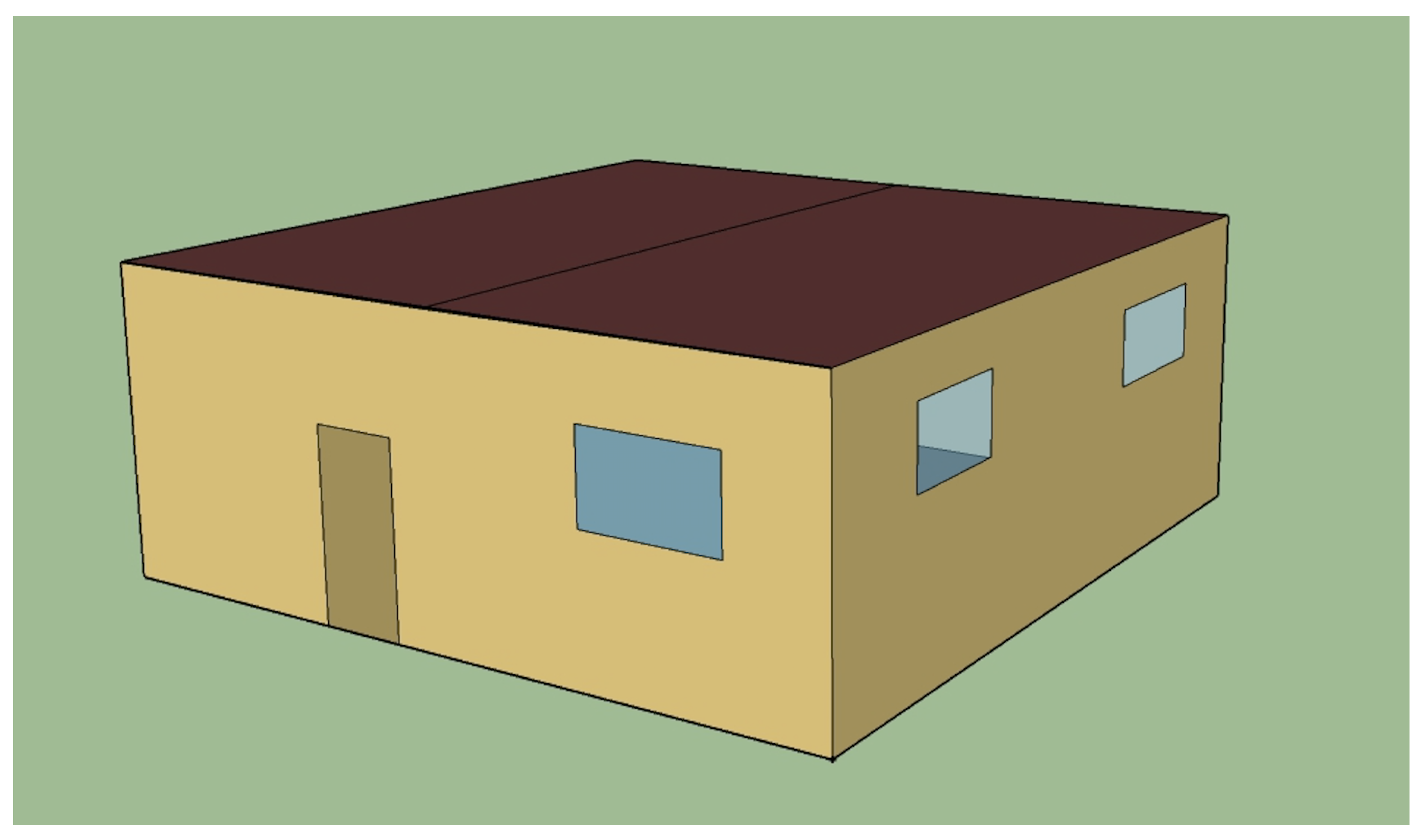
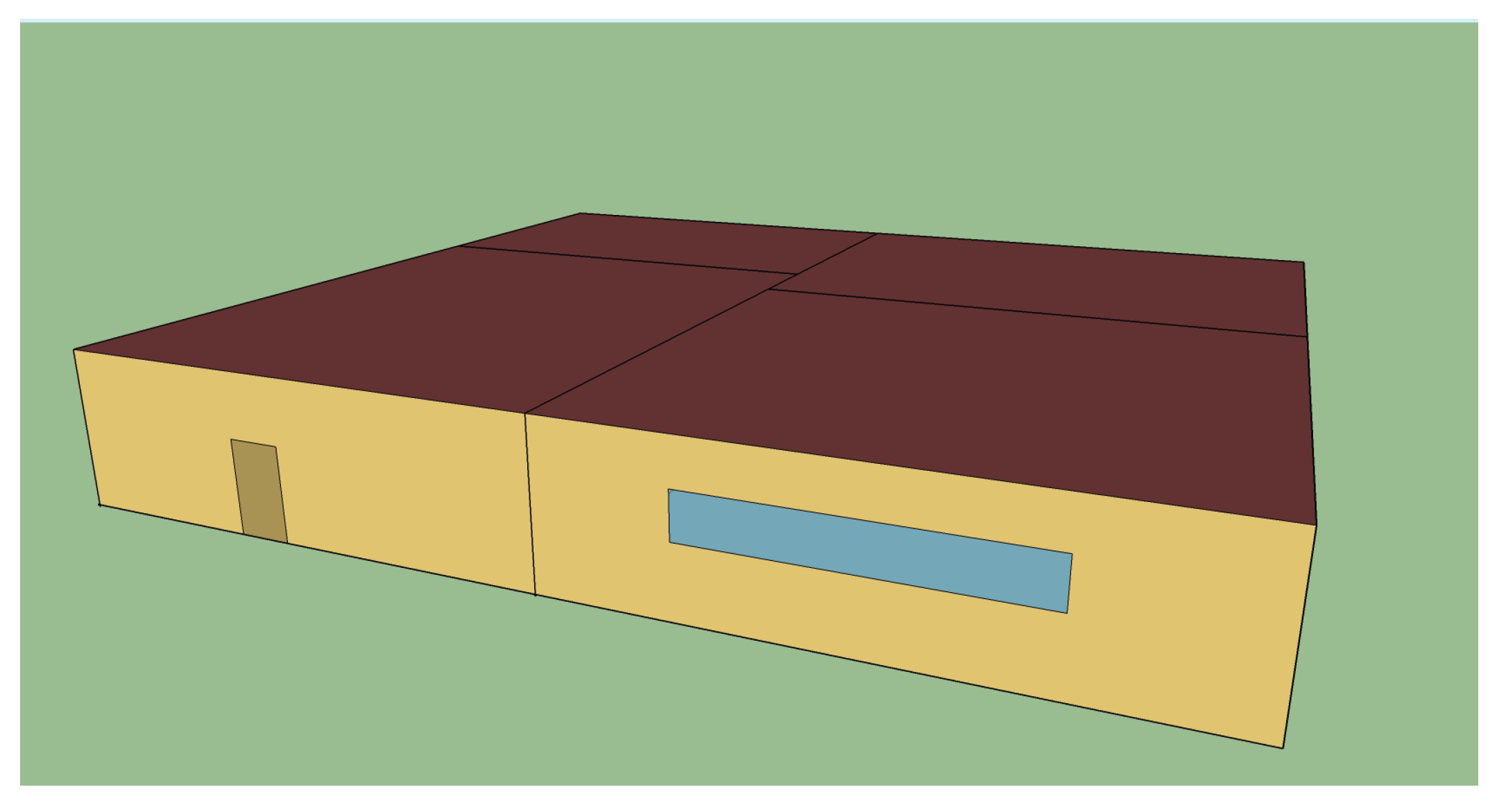
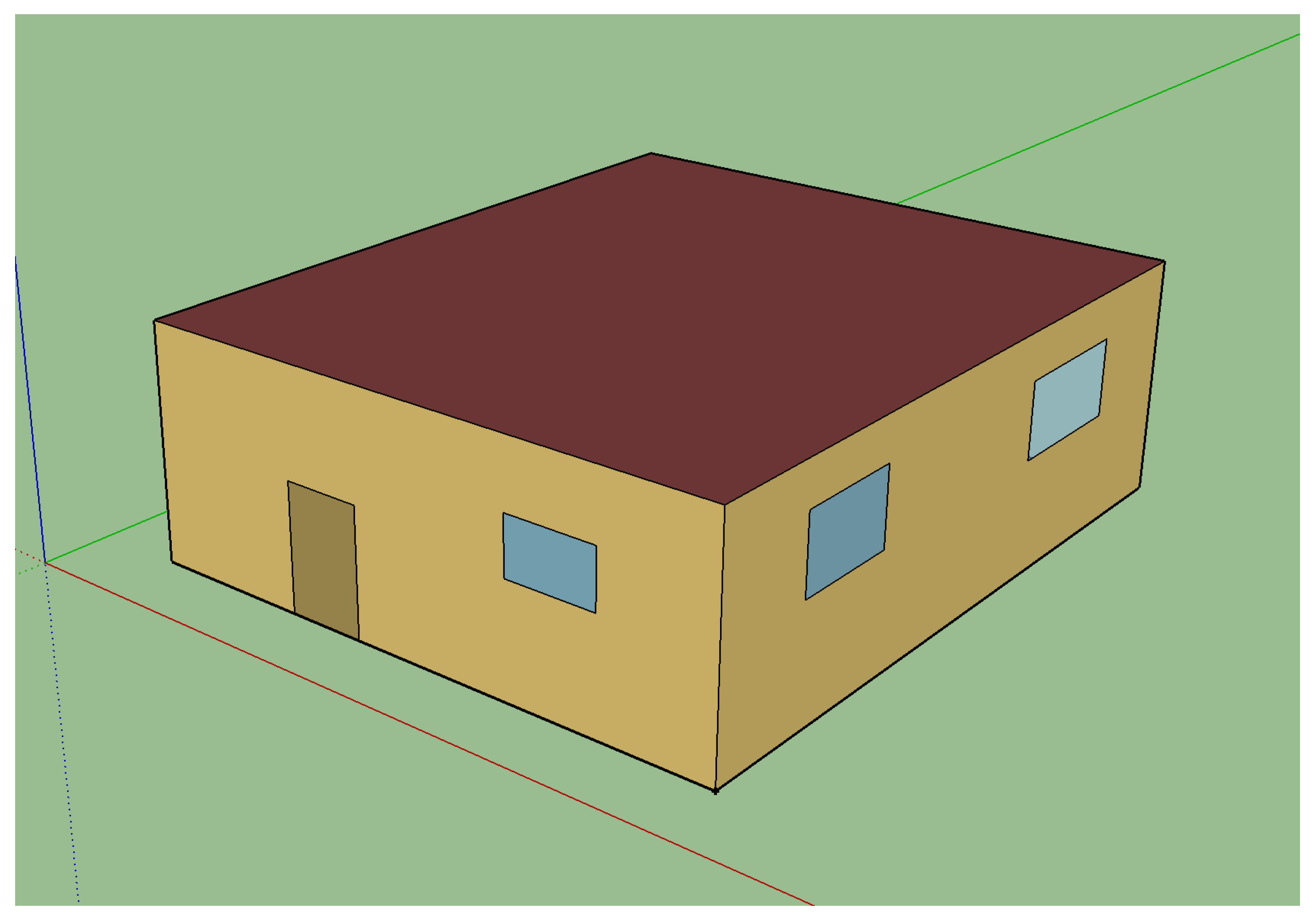
The residential building model used in the analysis was constructed in Sketchup (Computer-aided design (CAD) software) [17] and then applied using OpenStudio [18] and EnergyPlus software to run a year long simulation. EnergyPlus is only used for the simulation of the data set for each construction build we do, and then we try to best find a model to fit that data set. The location used in this study is Santa Barbara, California. The outdoor temperature for Santa Barbara is obtained from the Department of Energy EnergyPlus website for the year 2009. The model zone of a building, as seen in Figure 1 has dimensions of 7.72 m × 7.72 m × 3.046 m with an approximate volume of 181.5 m. The building has three windows and one door. All the material used is based on ASHRAE 189.1 standard corresponding to the location of the test area.
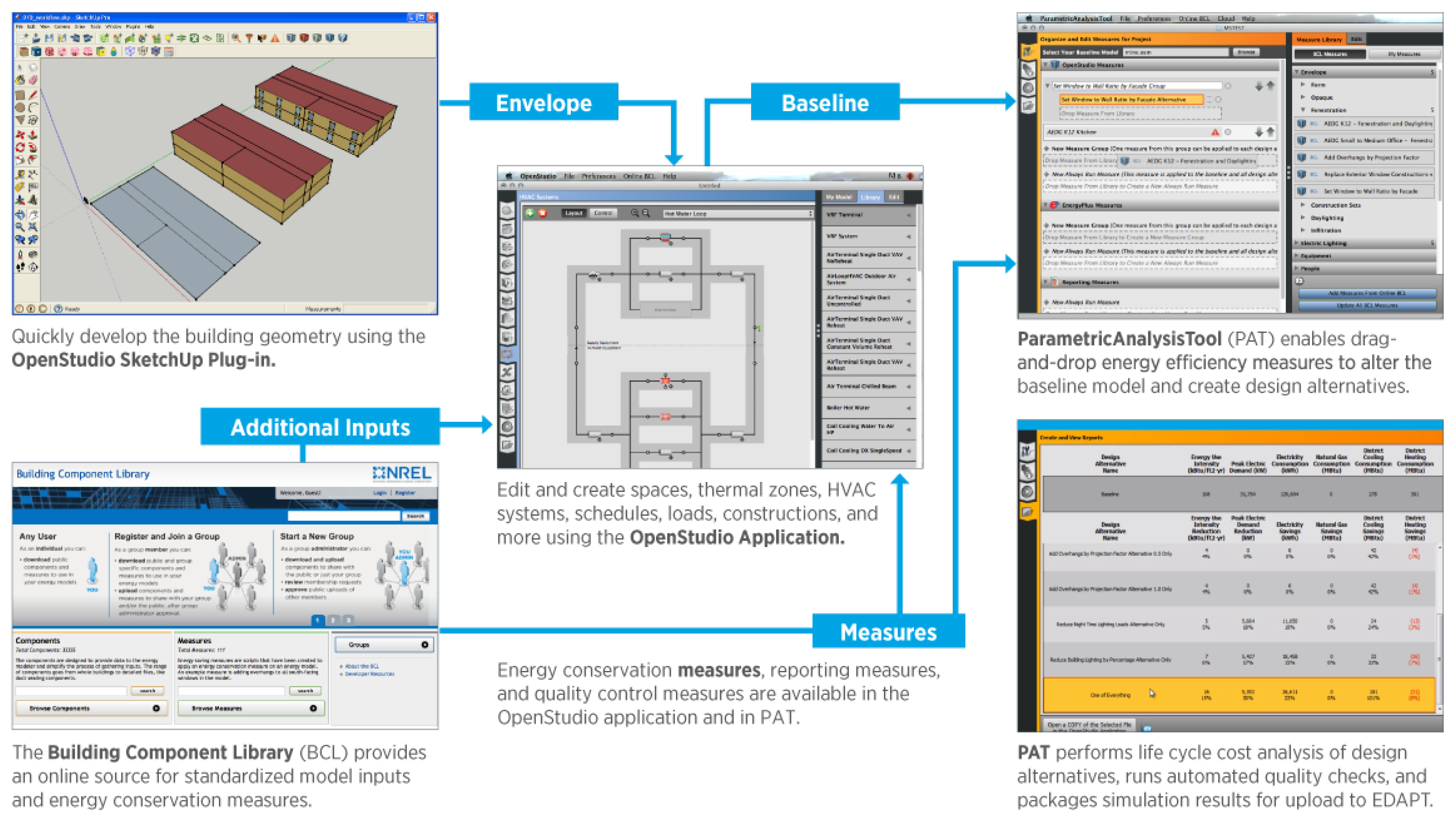
In OpenStudio, a wide-variety of conditions such as setpoints, occupant schedules, HVAC equipment, loads, and more (see Figure 2) can be specified. We first developed the nominal, no-actuation, no-load model, that enables us to parameterize important physical concepts such as the thermal mass by turning off all thermal loads. The model outputs were compared with a reduced order model the development of which we describe next.
4. Results
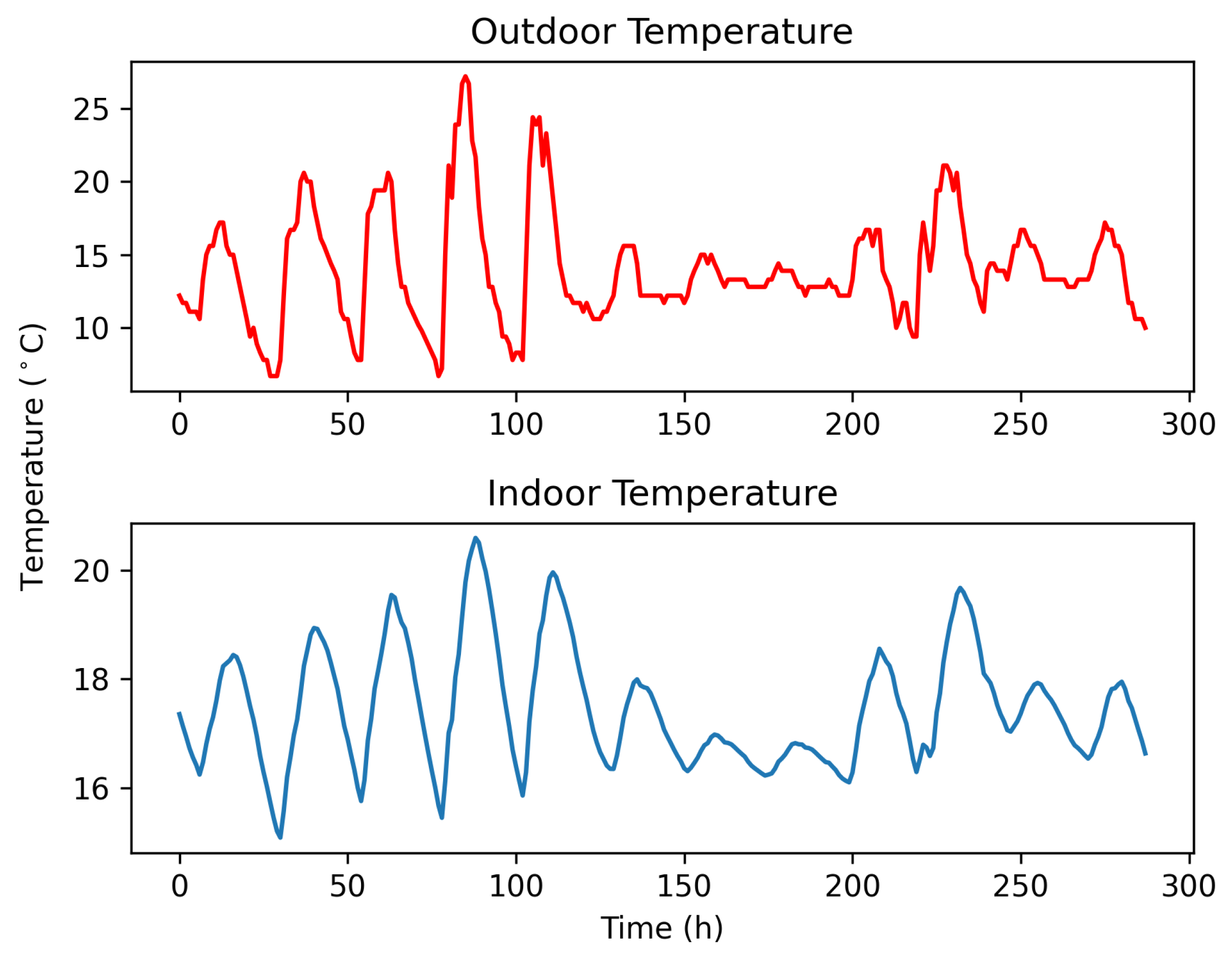
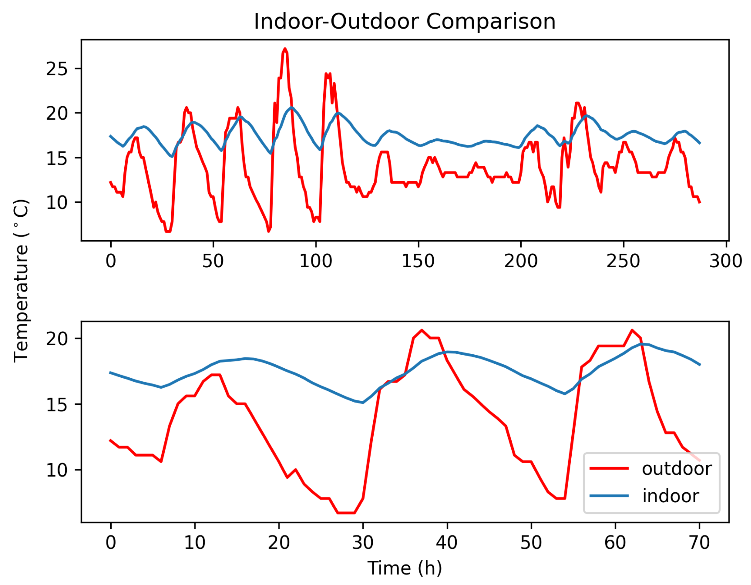
In this section, we report results obtained using a single-zone model and multi-zone. In OpenStudios we turned off all interior loads such as electrical loads and human schedule paterns for each particular space. We kept the thermal properties of heat transport according the each specific space type standards. In order to illustrate some of the complexity of temperature changes, in Figure 3 and Figure 4 we provide the indoor and outdoor temperature plots for our observation period in these simulations of 286 operational hours. There is a noticeable shift (delay) between the peaks of temperature between the outdoor and indoor temperatures. Control of the shift can be done, e.g., by the old fashioned manual implementation of opening the window before the sun is out and closing it afterwords in order to cool the home. However, the complexity of the delay timing indicates a system on chip control would be better in determining the exact times for such action, especially if the actuation is done using non-standard means such as active thermal mass.
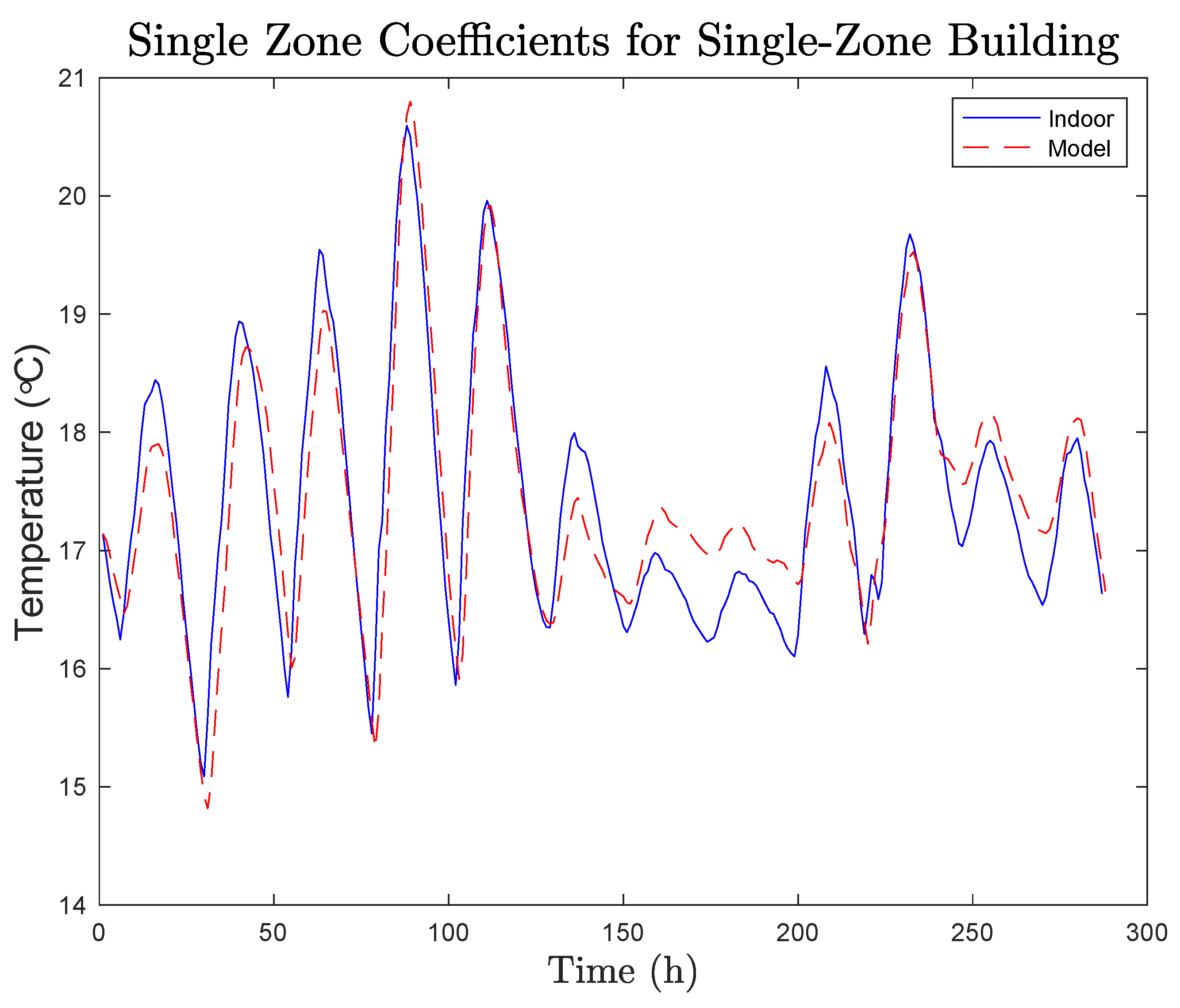
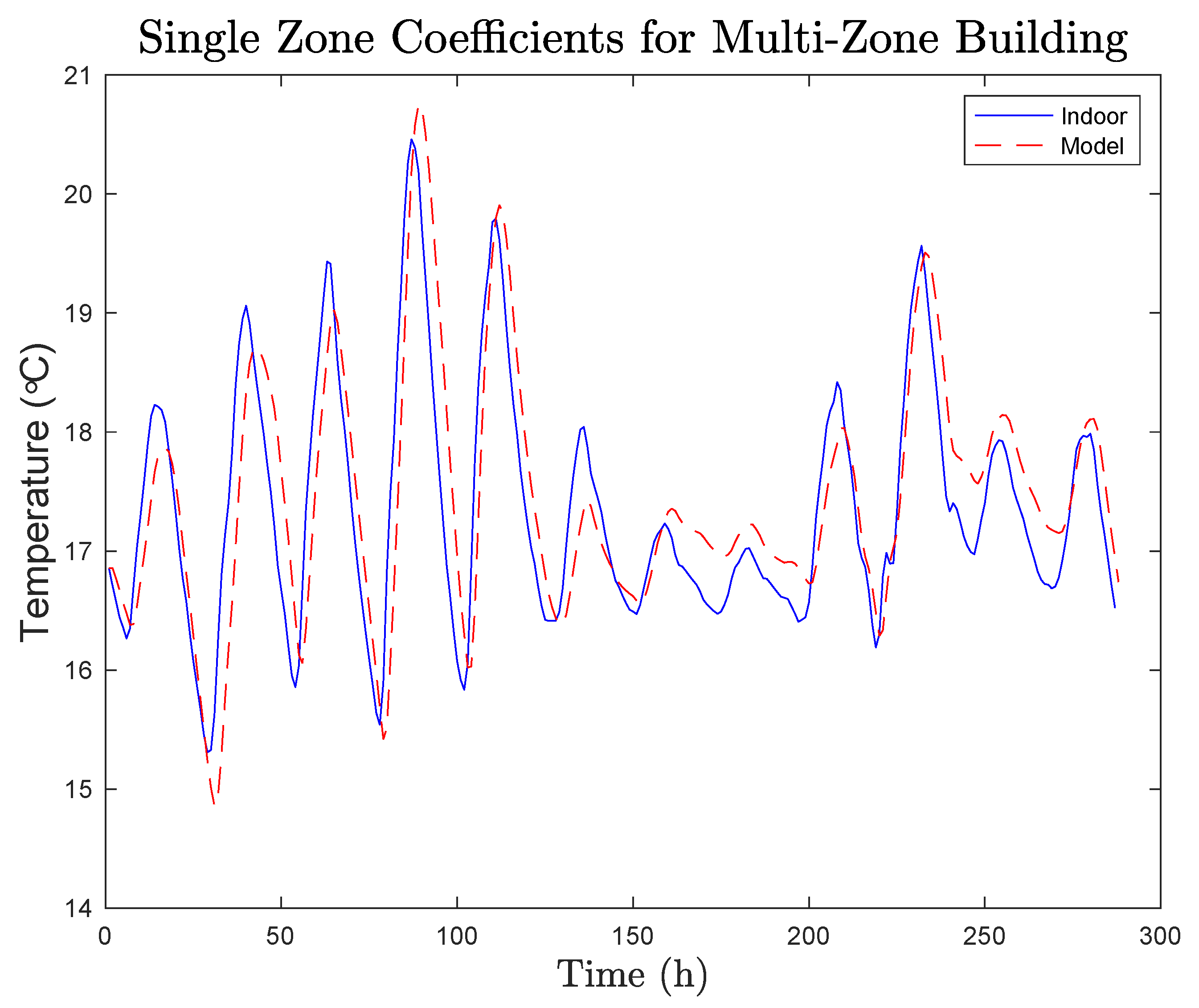
Once implement the grid parameter search in order to get the optimal coefficients described in Equation (9). The modeled indoor temperature compared to the “actual” indoor temperature from single zone building simulation from the EnergyPlus is shown in Figure 5. The percentage error found between the actual indoor temperature from simulation to our model is using Equation (11) to calculate error. This initial result is promising but we can extend it even further.
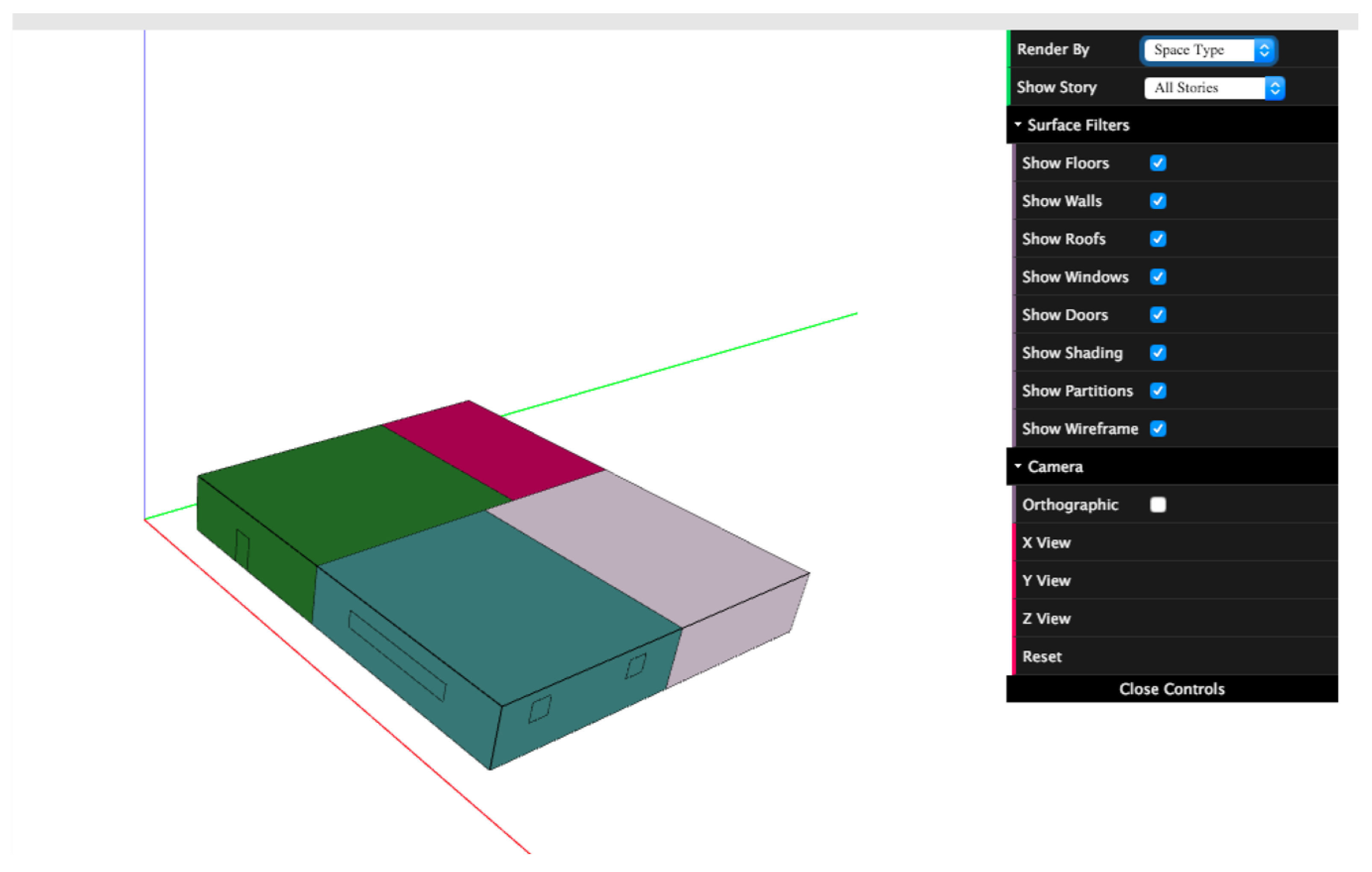
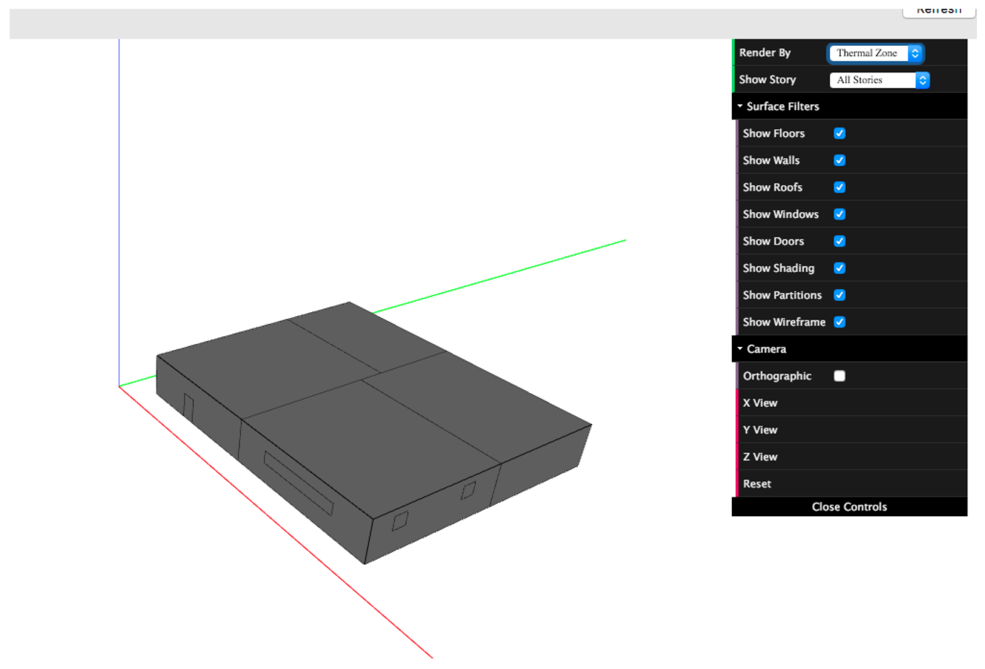
In order to better represent a model of a “real“ building or house structure, we need to investigate different properties within each particular space. We provide Sketchup and OpenStudio visual constructions in Figure 6, Figure 7 and Figure 8. Figure 7 is defined in OpenStudio after the construction was made, where each definition of a new space type will have it’s own unique properties. Each different space type will represent certain properties associated such as load, schedule of use, and even amount of airflow through the given area [19]. Zoning based on thermal properties of neighboring spaces based on Koopman operator methods was done in [20]. Since we have four different space types, we compute one thermal zone for the entire building which is illustrated in Figure 8. This one thermal zone is used in the EnergyPlus simulation as our true indoor temperature.
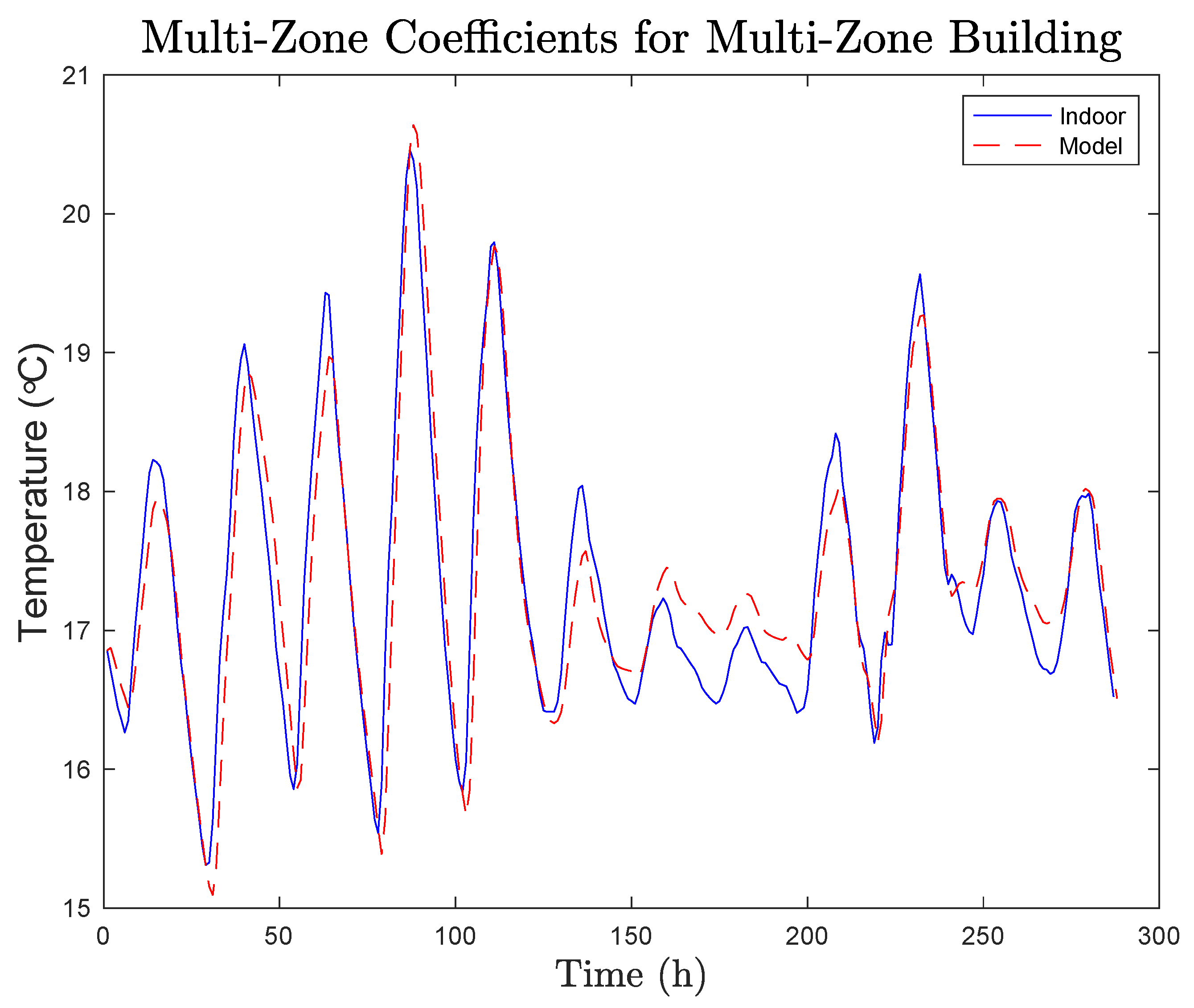
In Figure 9, we see that the proposed model performance is similar, with a difference from the “true” indoor temperature obtained using EnergyPlus. Even with having one thermal zone but four different spaces in a house, we see that the model will still capture the temperature regardless of the thermal properties between the spaces. In this sense, the reduced order model recognizes the homogenized coefficients such as the thermal mass for the whole building, indicating that the modeling can be done using a systematic layered approach, where both single zone and multi zone reduced order models are constructed.
Using the optimized parameters we found for a single zone building (Figure 5), we explored how well would that model do if we changed the construction parameters (i.e., more space types) while keeping the construction build material the same. In order to preform this test, we took the EnergyPlus simulation data from a multi-zone building (Figure 6) and tried to fit our model to it. In this experiment our model has never fit multiple zones and was not initial exposed to it, so this particular data set would be unique. Our model ended up preforming just as google as the single zone model on the single zone building, getting an astonishing percent difference of , seen in Figure 10.
5. Discussion
The result of this work provides framework for reduced order models to be implemented on embedded system on chip platforms. Studies have shown that retrofitting and introducing smart technology in buildings is the future for low energy consumption refs. [21,22].
Optimization of our coefficients in Equation (9) was an important factor in order to come up with the best model for our simulation results. It can be seen from our results that we can use the single zone model parameters that we fit and apply it to the same construction type regardless if more space types are added. It is better to fit the model parameters once we are exposed to a new construction such as adding more space types, this will make the model preform better which we saw when we refit our model to adjust to multi-zones.
In order to better understand the physical properties of our equation we examine Equation (10) closer to see what each parameter represents. The thermal mass influences the term strongly. Thermal mass is a very important aspect in buildings due to it being the main source of absorption of outside and inside thermal and passive control of the living space inside. The thermal mass is influenced by the physical structure of the walls of the building, because of the varying ability of the material to absorb and store heat energy. For example, a lot of thermal energy is needed to change the heat inside a building that has been constructed out of brick, due to the fact that the density of the material is high. In fact, any material that has greater thermal mass can store more heat and therefore it will take longer to release the thermal energy after the heat source or the sun is gone. Studies has shown maintaining healthy and comfortable conditions inside a residential building without causing high energy consumption can be implemented by using high thermal mass build material like concrete instead of lightweight timber [23,24].
Thermal insulation affects the “damping term” . It is used to reduce heat loss or gain by providing a barrier between areas that are significantly different in temperature. Insulation is commonly added between the outside walls and inside walls of the house, this is what provides that barrier of protection from the sun. Insulation and thermal mass both slow down the movement of heat between exterior and interior space. Insulation is used when a desired temperature differential is wanted between the indoor and outdoor space. Thermal mass is inertial, as it involves a substance that will slowly take on heat and then slowly release it over time [25].
Heat conduction affects the term. Thermal conduction happens when internal energy or heat is transferred by collision of particles and movement of electrons. Material within the walls have different heat conduction properties. The coefficient affects is in a sense a “global” heat conduction coefficient. Changing the materials in the walls affects both the thermal mass, and the thermal conduction term.
Thermal radiation, the heat transferred by electromagnetic waves such as the visible light or transfer of heat within or through two bodies affects the term in our equation. It was shown in [26] that radiation heat transfer results in an increase in the heat transfer rate reflecting significant radiation effects that contribute to less thermal resistance.
We note that the coefficients above are also affected by factors such as the orientation of the building. Thus, various physical and design considerations affect the coefficients in a heterogeneous way. Roughly, thermal mass affects , insulation affects , heat conduction coefficients , and thermal radiation . The above ROM (9) reduces computational complexity, from a computationally expensive EnergyPlus simulation to the simple model that can be implemented using embedded controllers and has all the essential physics encoded in its coefficients. Having ROM’s it is also easier to understand the nature of systems due to its simplicity.
Future Work
The proposed model also has some improvements that can be made. These improvements are adding load actuation to it, in terms of heating and cooling. This would be a easy addition to the model by adding another set of coefficients to our equation and doing another grid search for that new model parameter. The methodology described in [27,28], using occupancy based control would be a great implementation to our model for load actuation. This of course increases the model size in terms of having to search for more than three coefficients but now having to search for four or five, however this will still be faster than any EnergyPlus simulation.
We also mentioned system on chip capabilities and this is where the model would fit well. If we have real data from a residential building, we would be able to try and fit our model to that particular building. This system could live on the thermostat and recalculate if needed but after doing an initial calculation, the building itself will not change it’s orientation, size or construction type. Therefore one calculation would be needed to best fit the model to the real building and then let the thermostat regulate the actuation of the heating and cooling system as discussed above.
6. Conclusions
In this paper, we proposed a reduced order modeling methodology based on the backing of Koopman operator theory. The methodology leads to linear second order zone models featuring coefficients related to global physical properties of the space, such as the thermal mass. In fact, our effort can be seen as a way to define thermal mass for a zone as the coefficient in the reduced order model.
We tested the approach using simulated data from Energy Plus model for single and multi-zone buildings and found that optimized coefficients provide a good match of the reduced order model with the data. Building materials can affect the reduced order model coefficients substantially, illuminating their role in performance and efficiency of the thermal design of a building. In the Appendix A we present results of reduced order model coefficients with a variety of building materials, showing their effect on physical coefficients. From the results, it is evident that the variation of the thermal mass coefficient can be substantial, almost an order of magnitude. The damping coefficient and the “thermal stiffness” are affected less. In all the cases, the optimal coefficients provided for a good match with the Energy Plus data.
The low complexity, high accuracy reduced order models developed here can be used in development of controllers with standard actuation, but also non-standard, such as the active thermal mass actuation.
Author Contributions
Conceptualization, L.B. and I.M.; methodology, software, validation, data curation, writing—original draft preparation, writing—review & editing, L.B.; supervision, I.M. All authors have read and agreed to the published version of the manuscript.
Funding
This research was made possible by the generous gift from the Zaleski Foundation and particle funding from the ARO-MURI grant W911NF-17-1-0306.
Acknowledgments
The authors are grateful to the anonymous reviewers for their helpful comments and questions.
Conflicts of Interest
The authors declare no conflict of interest. The funders had no role in the design of the study; in the collection, analyses, or interpretation of data; in the writing of the manuscript, or in the decision to publish the results.
Appendix A. Variation of Coefficients of the Reduced Order Model with Different Materials
Appendix A.1. Standard Model
We created test models in OpenStudio with different structural materials (steel and brick) and different wall material. The size of the test building is 11.86 m × 13.99 m × 4.57 m and will have three windows and one door.
Figure A1.
The sketchup model used for varying internal parameters.

We used the total of 288 hourly data points. In the tables below we show Energy Plus model construction settings.

Table A1.
Standard model construction settings.
| Name | Material | External Wall Setting |
|---|---|---|
| Standard Model | 1/2in gypsum Wall insulation [39] MAT-sheath | Steel-framed |
For the standard model, we observed: , , . With an error of and the model read
Appendix A.2. Brick Model
The brick design used four different cases of materials showm in Table A2.
Table A2.
Brick case study construction layout.
| Name | Material | External Wall Setting |
|---|---|---|
| Brick Model | 1in stucco 8in concrete 1/2 gypsum Wall insulation [40] | Brick-framed |
| Brick and Insulation | 1in stucco 8in concrete 1/2 gypsum Wall insulation [40] Wall insulation [40] | Brick-framed |
| Brick, Insulation, and Gypsum | 1in stucco 8in concrete 1/2 gypsum Wall insulation [40] Wall insulation [40] 1/2in gypsum | Brick-framed |
| Brick, Insulation, and Concrete | 1in stucco 8in concrete 1/2 gypsum Wall insulation [40] Wall insulation [40] 8in concrete | Brick-framed |
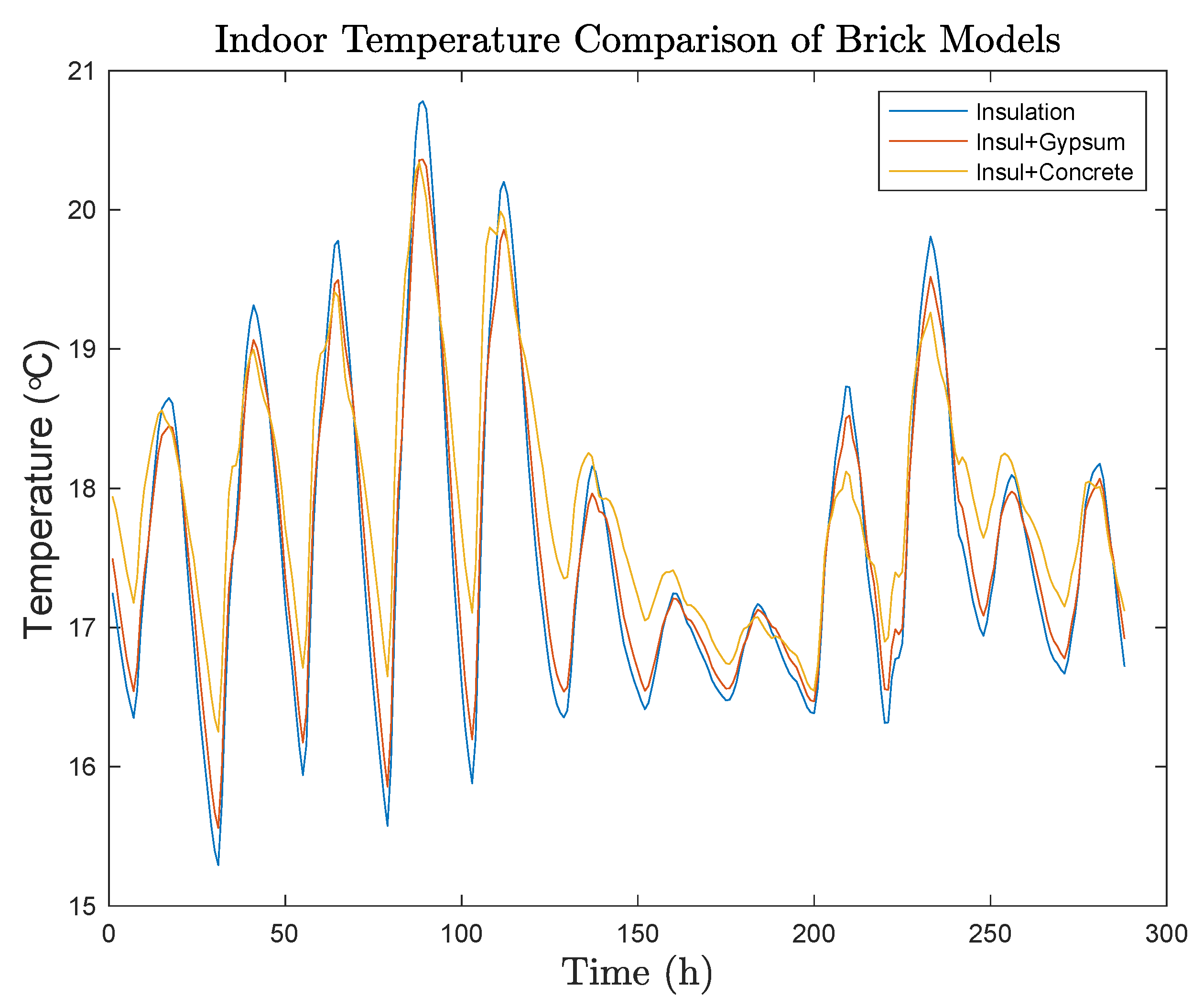
Figure A2.
Comparison of the indoor temperature for the three different internal structures of the model.
Figure A2.
Comparison of the indoor temperature for the three different internal structures of the model.

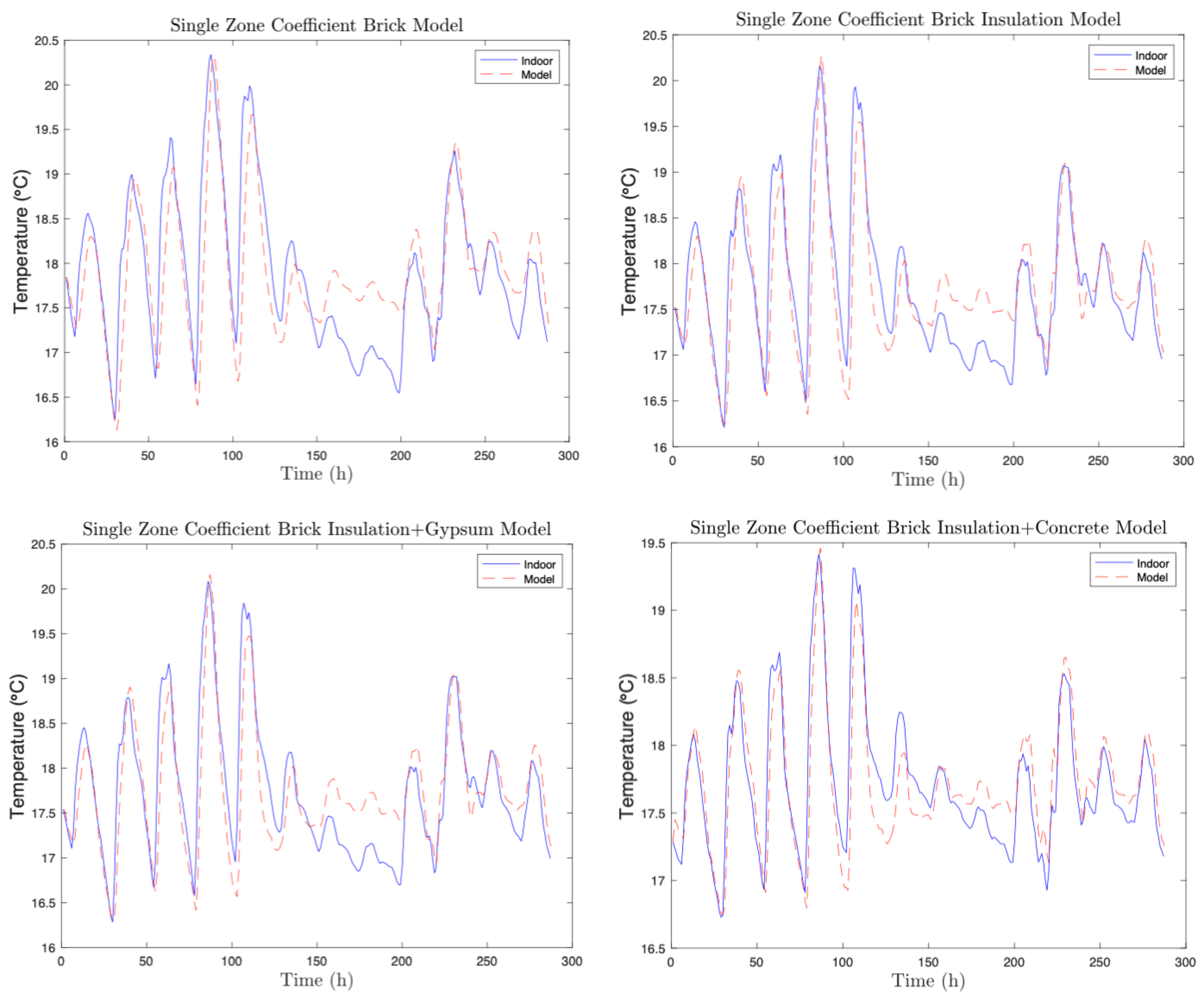
Figure A3.
Second order model plot of the four test cases with varying brick construction parameters defined in Table A2.
Figure A3.
Second order model plot of the four test cases with varying brick construction parameters defined in Table A2.

For the pure brick model the coefficients were found to be, , , and . Error = 7.7222%, and the model read
For the brick mode with added insulation the coefficients were found to be, , , and . Error = 6.0809% and the model reads
For the brick mode with added insulation and gypsum teh coefficients were found to be, , , and . Error = 5.9672% and the model read
For the brick mode with added insulation and concrete the coefficients were found to be, , , and . Error = 3.3882% and the model reads
References
- Hoicka, C.E.; Parker, P. Assessing the adoption of the house as a system approach to residential energy efficiency programs. Energy Effic. 2018, 11, 295–313. [Google Scholar] [CrossRef]
- Littooy, B.; Loire, S.; Georgescu, M.; Mezić, I. Pattern recognition and classification of HVAC rule-based faults in commercial buildings. Big Data (Big Data). In Proceedings of the 2016 IEEE International Conference, Melaka, Malaysia, 28–29 November 2016; pp. 1412–1421. [Google Scholar]
- Georgescu, M.; Mezić, I. Building energy modeling: A systematic approach to zoning and model reduction using Koopman Mode Analysis. Energy Build. 2015, 86, 794–802. [Google Scholar] [CrossRef]
- Mezic, I. Dynamics of System of Systems and Applications to Net Zero Energy Facilities; Technical Report; University of California-Santa Barbara Santa Barbara United States: Santa Barbara, CA, USA, 2017. [Google Scholar]
- Bureau, U.S.C. Number of Housing Units in the United States from 1975 to 2017. 2018. Available online: https://www.statista.com/statistics/$240267$/number-of-housing-units-in-the-united-states/ (accessed on 20 July 2019).
- Ford, R.; Pritoni, M.; Sanguinetti, A.; Karlin, B. Categories and functionality of smart home technology for energy management. Build. Environ. 2017, 123, 543–554. [Google Scholar] [CrossRef] [Green Version]
- Mezić, I. Spectral properties of dynamical systems, model reduction and decompositions. Nonlinear Dyn. 2005, 41, 309–325. [Google Scholar] [CrossRef]
- Boskic, L.; Brown, C.N.; Mezić, I. Koopman mode analysis on thermal data for building energy assessment. Adv. Build. Energy Res. 2020, 1–15. [Google Scholar] [CrossRef]
- Masaki, I.; Susuki, Y.; Mezic, I.; Ishigame, A. An LC-Circuit Model for Dynamics of In-Building Heat Transfer across Atrium Space. In Proceedings of the IOP Conference Series: Earth and Environmental Science, Malang City, Indonesia, 12–13 March 2019; Volume 238, p. 012012. [Google Scholar] [CrossRef] [Green Version]
- May-Ostendorp, P.; Henze, G.P.; Corbin, C.D.; Rajagopalan, B.; Felsmann, C. Model-predictive control of mixed-mode buildings with rule extraction. Build. Environ. 2011, 46, 428–437. [Google Scholar] [CrossRef]
- Avci, M.; Erkoc, M.; Rahmani, A.; Asfour, S. Model predictive HVAC load control in buildings using real-time electricity pricing. Energy Build. 2013, 60, 199–209. [Google Scholar] [CrossRef]
- Hazyuk, I.; Ghiaus, C.; Penhouet, D. Optimal temperature control of intermittently heated buildings using Model Predictive Control: Part I–Building modeling. Build. Environ. 2012, 51, 379–387. [Google Scholar] [CrossRef]
- Mezić, I.; Banaszuk, A. Comparison of systems with complex behavior. Phys. D Nonlinear Phenom. 2004, 197, 101–133. [Google Scholar] [CrossRef]
- Mezić, I. Analysis of fluid flows via spectral properties of the Koopman operator. Annu. Rev. Fluid Mech. 2013, 45, 357–378. [Google Scholar] [CrossRef] [Green Version]
- Susuki, Y.; Mezic, I.; Raak, F.; Hikihara, T. Applied Koopman operator theory for power systems technology. Nonlinear Theory Its Appl. IEICE 2016, 7, 430–459. [Google Scholar] [CrossRef] [Green Version]
- Mauroy, A.; Mezić, I.; Susuki, Y. The Koopman Operator in Systems and Control: Theory, Numerics, and Applications; Springer: Berlin/Heidelberg, Germany, 2019. [Google Scholar]
- SketchUp Pro 2018. 2017. Available online: https://www.sketchup.com/products/sketchup-pro (accessed on 1 September 2018).
- Openstudio. National Laboratory of the U.S. DOE. 2017. Available online: https://www.openstudio.net/ (accessed on 1 September 2018).
- OpenStudio. 12-1 Space Types in OpenStudio. Available online: https://energy-models.com/training/12-1-space-typesopenstudio (accessed on 1 September 2018).
- Georgescu, M.; Eisenhower, B.; Mezic, I. Creating zoning approximations to building energy models using the Koopman operator. Proc. Simbuild 2012, 5, 40–47. [Google Scholar]
- Prada, M.; Prada, I.F.; Cristea, M.; Popescu, D.E.; Bungău, C.; Aleya, L.; Bungău, C.C. New solutions to reduce greenhouse gas emissions through energy efficiency of buildings of special importance–Hospitals. Sci. Total Environ. 2020, 718, 137446. [Google Scholar] [CrossRef] [PubMed]
- Sittón-Candanedo, I.; Alonso, R.S.; García, O.; Munoz, L.; Rodríguez-González, S. Edge Computing, IoT and Social Computing in Smart Energy Scenarios. Sensors 2019, 19, 3353. [Google Scholar] [CrossRef] [PubMed] [Green Version]
- Kuczyński, T.; Staszczuk, A. Experimental study of the influence of thermal mass on thermal comfort and cooling energy demand in residential buildings. Energy 2020, 195, 116984. [Google Scholar] [CrossRef]
- Sharaf, F. The impact of thermal mass on building energy consumption: A case study in Al Mafraq city in Jordan. Cogent Eng. 2020, 7, 1804092. [Google Scholar] [CrossRef]
- Çengel, Y.A.; Boles, M.A. Thermodynamics an Engineering Approach, 8th ed.; The McGraw-Hill Companies, Inc.: New York, NY, USA, 2007. [Google Scholar]
- Antar, M.A. Thermal radiation role in conjugate heat transfer across a multiple-cavity building block. Energy 2010, 35, 3508–3516. [Google Scholar] [CrossRef]
- Krarti, M. Evaluation of occupancy-based temperature controls on energy performance of KSA residential buildings. Energy Build. 2020, 220, 110047. [Google Scholar] [CrossRef]
- Wang, C.; Pattawi, K.; Lee, H. Energy saving impact of occupancy-driven thermostat for residential buildings. Energy Build. 2020, 211, 109791. [Google Scholar] [CrossRef]
Figure 1.
The sketchup model construction used for EnergyPlus as the single zone house.

Figure 2.
OpenStudio Application work flow, displays how a sketchup model can be loaded in and configured prior to running a EnergyPlus simulation.
Figure 2.
OpenStudio Application work flow, displays how a sketchup model can be loaded in and configured prior to running a EnergyPlus simulation.

Figure 3.
Hourly indoor-outdoor simulation temperature data during 2/26 to 3/09.

Figure 4.
Indoor-outdoor temperature closeup of a 72 h window within the data above.

Figure 5.
Single zone coefficients fit to a single zone building using the second order model.

Figure 6.
The multi-zone sketchup model construction used for EnergyPlus.

Figure 7.
OpenStudio diagram of the four different space type declarations, where each different space type will have different properties such as electrical usage.
Figure 7.
OpenStudio diagram of the four different space type declarations, where each different space type will have different properties such as electrical usage.

Figure 8.
Single thermal zone representation of a multi-zone building.

Figure 9.
Second order model for indoor air temperature of a multi-zone building.

Figure 10.
Single zone coefficients fit to a multi-zone building using the second order model.

Publisher’s Note: MDPI stays neutral with regard to jurisdictional claims in published maps and institutional affiliations. |
© 2021 by the authors. Licensee MDPI, Basel, Switzerland. This article is an open access article distributed under the terms and conditions of the Creative Commons Attribution (CC BY) license (http://creativecommons.org/licenses/by/4.0/).
Share and Cite
MDPI and ACS Style
Boskic, L.; Mezic, I. Control-Oriented, Data-Driven Models of Thermal Dynamics. Energies 2021, 14, 1453. https://doi.org/10.3390/en14051453
AMA Style
Boskic L, Mezic I. Control-Oriented, Data-Driven Models of Thermal Dynamics. Energies. 2021; 14(5):1453. https://doi.org/10.3390/en14051453
Chicago/Turabian StyleBoskic, Ljuboslav, and Igor Mezic. 2021. "Control-Oriented, Data-Driven Models of Thermal Dynamics" Energies 14, no. 5: 1453. https://doi.org/10.3390/en14051453
Note that from the first issue of 2016, this journal uses article numbers instead of page numbers. See further details here.