Article

Modelling and Control of a Grid-Connected RES-Hydrogen Hybrid Microgrid

1
Dipartimento Energia ”Galileo Ferraris”, Politecnico di Torino, Corso Duca degli Abruzzi 24, 10129 Torino, Italy
2
Energy Center Lab (EC-L), Politecnico di Torino, via Paolo Borsellino 38/16, 10138 Torino, Italy
3
Centre of Expertise Energie, Hanze University of Applied Sciences, Zernikelaan 17, 9747 AA Groningen, The Netherlands
*
Author to whom correspondence should be addressed.
Energies 2021, 14(6), 1540; https://doi.org/10.3390/en14061540
Submission received: 31 December 2020 / Revised: 22 February 2021 / Accepted: 4 March 2021 / Published: 11 March 2021

Abstract

:
This paper proposes a Hybrid Microgrid (HμG) model including distributed generation (DG) and a hydrogen-based storage system, controlled through a tailored control strategy. The HμG is composed of three DG units, two of them supplied by solar and wind sources, and the latter one based on the exploitation of theProton Exchange Membrane (PEM) technology. Furthermore, the system includes an alkaline electrolyser, which is used as a responsive load to balance the excess of Variable Renewable Energy Sources (VRES) production, and to produce the hydrogen that will be stored into the hydrogen tank and that will be used to supply the fuel cell in case of lack of generation. The main objectives of this work are to present a validated dynamic model for every component of the HμG and to provide a strategy to reduce as much as possible the power absorption from the grid by exploiting the VRES production. The alkaline electrolyser and PEM fuel cell models are validated through real measurements. The State of Charge (SoC) of the hydrogen tank is adjusted through an adaptive scheme. Furthermore, the designed supervisor power control allows reducing the power exchange and improving the system stability. Finally, a case, considering a summer load profile measured in an electrical substation of Politecnico di Torino, is presented. The results demonstrates the advantages of a hydrogen-based micro-grid, where the hydrogen is used as medium to store the energy produced by photovoltaic and wind systems, with the aim to improve the self-sufficiency of the system.

1. Introduction

During the last years, the number of research and development projects considering as main energy sources the so called Variable Renewable Energy Sources (VRES), such as photovoltaic (PV) and wind (WD), increased. These projects are largely driven by government regulations. Thus, the increase of RES challenged scientists and technicians to study and implement new strategies to improve the operation and stability of energy systems, and, in the meanwhile, to decrease the dependency by fossil fuels or, under a different point of view, lessening the emission of greenhouse gases [1]. However, the intermittency typical of VRES introduces an additional risk which could compromise the successful satisfaction of the load [2]. Therefore, the electrical system needs flexibility, that can be provided in different ways. In [3], the flexibility is guaranteed by coordinating several Peltier Effect regrigerator [4]. In [5] the flexibility is provided by a compression-based refrigerator, whereas in [6] the exploitation of distributed multi-energy system is suggested as form of flexibility for the electrical grid. In this context, Power-to-X (P2X) technologies, such as Power-to-Gas (P2G), Power-to-Fuels (P2F), and Power-to-Heat (P2H), are gaining a leading role for providing flexibility to the electricity grid, because (i) they are able to exploit the existing infrastructure (such as the gas network and district heating) and (ii) allow decarbonising other sectors using the produced commodities (i.e., gas, liquids and heat) starting from an excess of VRES [7]. Two of the above mentioned processes (i.e., P2G and P2F) are based on the production of green hydrogen that can be successively converted in methane or liquid fuels by combining it with CO2. However, this cannot determine the solution of the CO2 emission. The only way is to use as energy carrier the green hydrogen and make use of it as basic element for the future energy system: this perspective, even though was indicated as possibile and desiderable in the past (see for example [8]), is now is gaining a momentum. In particular, on the basis of the European Green Deal [9], the European Commission presented the EU Hydrogen Strategy [10], which includes two phases, having as objective to reach 6 GW of installed electrolysers up to the end of 2024 (with a production of up to 1 million tonnes of green hydrogen) and successively jump up to 40 GW at the end of 2030, with a production reaching 10 millions tonnes, to be compliant with the goal of covering around 14% of the European energy mix with green hydrogen [11]. In China, the definition of the different types of hydrogen has been debated and a recent standard reports their characteristics, by defining low-carbon hydrogen, clean hydrogen and renewable hydrogen on the basis on their specific emission and the origin of the electricity [12].
Several hydrogen-based energy projects around the world aimed or are aiming to study how to properly exploit the advantages from the coupling of RES-based power plants and hydrogen: taking as example the European Union, the activities in this topic are led by the Fuel Cells and Hydrogen Joint Undertaking (FCH JU) and, since its foundation in 2008, more than 220 projects have been propitiated [13]. This great interest is also due to the possibility to have a bi-directional conversion, i.e., from electricity to hydrogen (through electrolysers) and viceversa (by using fuel cells): this opens perspectives in which the hydrogen, properly stored, may be used as an energy buffer that, combined with electrolysers and fuel cells, could improve the self sufficiency of the prosumers, by reducing the grid dependency. With this scope, the hydrogen-based system is used as an Energy Storage System (ESS) and the prosumer plant can be seen as a Hybrid Micro-Grid (HμG).
A HμG may combine RES power plants, gas-based devices and energy storage capability. It can supply remote customers with clean and cost-effective electricity [14]: in fact, if properly designed, H μ Gs can be operated also in islanded way [15]. The structure to consider could be composed by a whole H2 energy system, which employs mainly fuel cells, electrolysers and hydrogen tanks. Therefore, to present these new hybrid systems as a potential solution, two main aspects have to be considered: (i) novel algorithms to manage the surplus of energy associated with RES, and (ii) new strategies of energy management, in order to drive the power flow calculation of hydrogen systems integrated into the H μ Gs [1].
In literature, the contributions on this topic focus on specific aspects of the system. For example, in [16], the author proposed the sizing of a hybrid plants (including photovoltaic and fuel cells) based on models included in the software HOMER. In [17], the authors evaluated the sizing of batteries and hydrogen energy storage for a real domestic load, but with infinite storage capacity. In [18] different meta-heuristic methods have been compared to optimally design an isolated H μ G. All the above contributions consider simulation time steps of one hour, which are good enough for energy evaluation, but cannot properly represent the dynamics. In [19], the time step is shorter (aroung 30 s), but the measurements of the electrical load were not based on real data and the response of electrolysers and fuel cells are based on simplified models. In [20], the authors proposed a model implemented on a real-time simulation, by considering a DC grid layout. Also in this case, a simplified response of the electrolyser and fuel cell is considered. Even though considering dynamic behaviour of the components, other contributions investigates specific aspects with small size components. For example, the authors in [21] presented a H μ G including an electrolyser and a fuel cell of size around 1kW. The same layout has been employed in [22] to investigate the use of Model Predictive Control in the energy management of the H μ G.
In this paper, a H μ G layout based on validated models of all the components is proposed. The implemented control strategy aims to reduce as much as possible the dependence from the main grid, to improve the self-sufficiency of the prosumer. The main contributions of the paper are: (i) the hydrogen-based components, whose sizes are higher than the ones previously considered for fast dynamic studies (8 kW for the electrolyser and 12.5 kW for the fuel cells), (ii) the use of a high-speed sampled real electrical load, which has been measured at Politecnico di Torino (Italy) and (iii) the validation of all the components of the system, based on real data. In particular, the validation data for the PEM fuel cell have been collected locally, whereas the validation data of the electrolyser operation have been collected remotely as in Reference [23] with high sampling frequency
The paper is organized as follows: Section 2 introduces the layout of the H μ G and the dynamic models of the components i.e., PV and WD generation systems, electrolyser, fuel cell and hydrogen tank. Section 3 shows the implemented control strategy, whereas Section 4 presents the simulation results with different case studies. Finally, the last section lists the concluding remarks.

2. HμG Modelling

2.1. HμG Layout

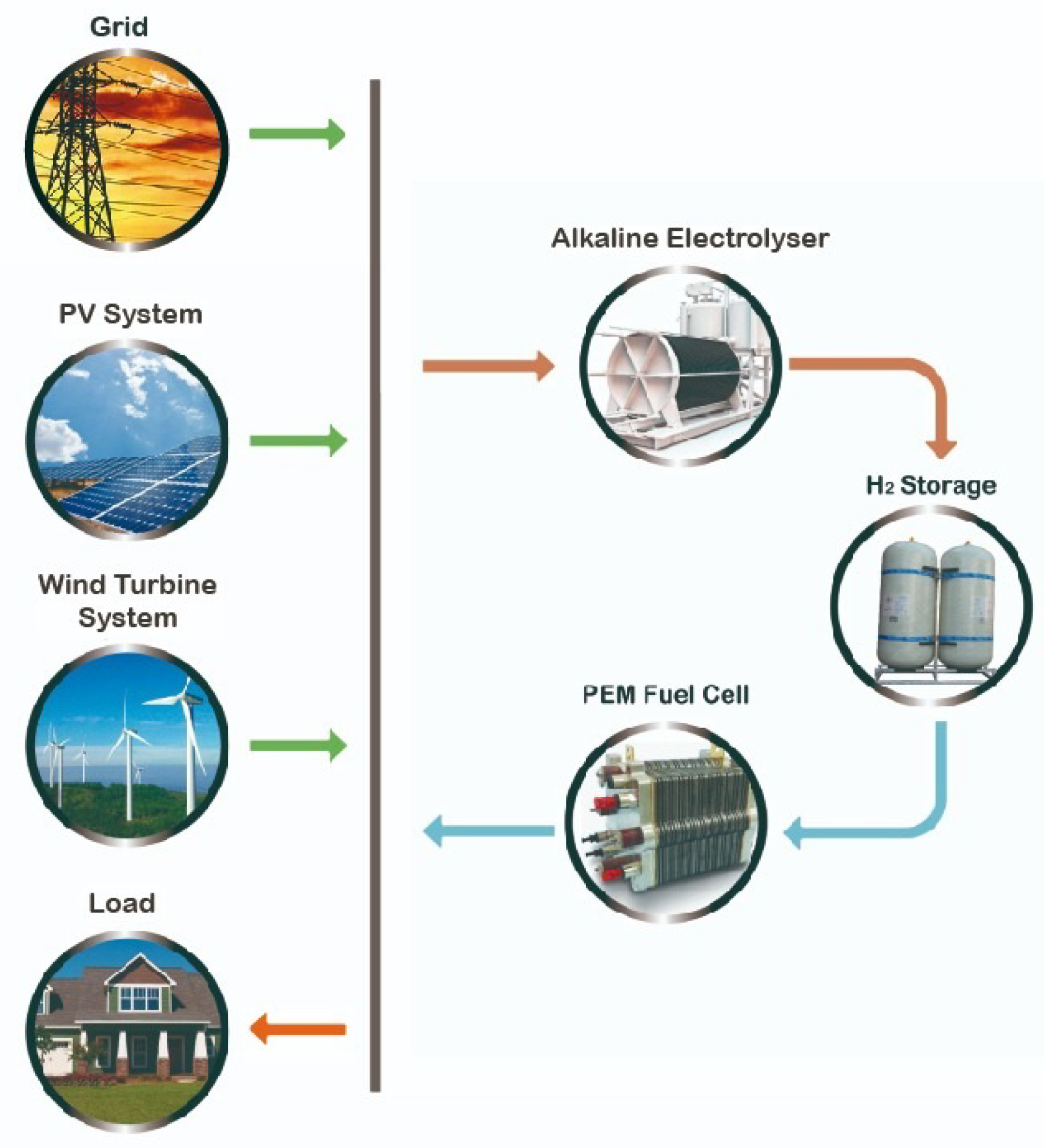
The HμG presented in this paper is composed of multiple generation sources, an EES, and a non-flexible load. The generation system is composed of a PV system, a WD generator and a Proton Exchange Membrane (PEM) fuel cell (FC). The ESS consists basically in a hydrogen storage tank (HST) coupled with an alkaline electrolyser (ELY). The ESS subsystem is connected to the non-flexible load and has enough capacity to supply the FC when needed.
A general model of hydrogen storage system is integrated to manage the production and consumption of energy from the electrolyser and the PEM FC respectively. The electrolyser is used to absorb rapidly the output power from RES and generates hydrogen as fuel for FCs [24,25].
The schematic diagram of the H μ G is presented in Figure 1. The sum of the demand and electrolyser power is equal to the sum of the grid contribution and the output power generated by WD and PV generators and PEM fuel cells.
Equation (1) represents the power balance in the H μ G:
P L O A D = P G R I D + P W D + P P V + P F C P E L Y
where P L O A D is the power demand, P G R I D is the power provided by the grid, P W D and P P V are the RES contributions, from the wind system and from the solar system respectively, P F C is the power produced by the PEM fuel cell and P E L Y the power consumed by the electrolyser.
In the following sections, a general description of the technical specifications for each component is presented. Furthermore, the models used to simulate each component are described, together with their testing and validation. All the components’ models and the overall H μ G system are simulated in Matlab Simulink®.

2.2. Load Demand

The load is considered to absorb only active power. The load profiles are loaded from a file. Two load profiles are considered in this work: (a) a synthetic load profile built with the aim to test the proper system operation and (b) a real load profile, obtained from real measurements.
The measurements were performed in a Medium Voltage (MV)/Low Voltage (LV) substation on a LV feeder supplying a data center at Politecnico di Torino on 18th and 19th June 2019. We used a high speed recorder Hioki 8880/20 MR with a direct connection to the feeder for voltage measurements and probes pico technology TA 167 for current measurements. The sampling time was set to 1 s.
The two load profiles are presented in Figure 2.

2.3. Wind Turbine System

One of the renewable generators of the H μ G is the wind turbine system. The turbine considered in the H μ G has a rated power of 15 kW, a rated speed of 15 m/s, a cut-in speed of 5 m/s and a cut-out speed of 30 m/s. The average daily elecrical production is about 8 kWh.

2.4. PV System

The second renewable generator of the H μ G is the PV system; it delivers a maximum of 23 kW at 1000 W/m 2 sun irradiance. The technical specifications of the PV system are summarized in Table 1.

2.5. Alkaline Electrolyser

Electrolysers produce hydrogen from water dissociation. For the H μ G described in this work, we modelled an alkaline electrolyser which, bytheway, it the most mature and available in the market [26].
In an alkaline electrolyser, the alkaline solution (usually based on KOH at 30% in weight) is used as electrolyte. The modelled electrolyser has rate power 8 kW and rate hydrogen flow equal to 1.255 Nm3/h, with pressure 12 barg and purity higher than 99.3%. The electrolyser comprises one stack of 8 kW, composed of 5 series-connected cells. The average efficiency is about 54.4% (low heating value). The electrolyser technical specifications are presented in Table 2.
The alkaline electrolyser model presented is related to an Advanced Alkaline electrolyser. In the electro-chemical model temperature and pressure depends on Faraday efficiency, whereas the temperature depends on current-voltage relation [27,28].
The model may forecast the cell voltage, the hydrogen production, Faraday efficiency and the electrolyser operating temperature [27]. In Figure 3 the block diagram of the sub-models is presented. The sub-models are described in detail in the next paragraphs.

2.5.1. Thermodynamic Sub-Model

The reversible voltage is defined as the minimum voltage that, applied to the water molecule, allows its separation. The reversible voltage U r e v is expressed in terms of the Gibbs Energy variation, as reported in Equation (2).
Δ G = Δ H T · Δ S
The Gibbs energy can be associated with reversible voltage and themoneutral cell voltage as shown in Equation (3).
U r e v = Δ G z · F
where the reversible voltage U r e v is measured in V and is sensible to reaction temperature and pressure, z the hydrogen molecule electrons, and F is the Faraday constant, equal to F = 96,485.3329 C/mol. The total energy demand Δ H refers to thermo-neutral cell voltage and it is expressed by Equation (4).
U t h = Δ H z · F

2.5.2. Electrical Sub-Model

The electrical sub-model allows the estimation of the voltage-current relationship. The model inputs are the electrical power and the stack temperature, whereas the output is the voltage-current couple for every stack cell at different temperatures [29].
The relationship of the electrical power on the electrolyser is given Equation (5):
W E L Y = N L E Y · I E L Y · U E L Y
where W E L Y is the consumed power in W, N E L Y is the of stack cell number, I E L Y is the stack current of the electrolyser in A, U E L Y and is the electrolyser cell voltage in V.
In Equation (5), the electrolyser cell voltage U E L Y represents an empirical I U model for electrolysers. The kinetics of the cell electrode are modeled with the I U curve, which includes the ohmic and stack temperature effects. The I U curve can be expressed by the sum of three terms, as reported in Equation (6): the reversible voltage U r e v , the activation voltage U a , and the ohmic overvoltage U o h m . All the terms are expressed in V [30].
U E L Y = U r e v + U a + U o h m
The first term of the right-side of Equation (6) represents the minimum voltage required to activate the ideal electrolyser cell, as expressed above in Equation (3). The second and third terms refer to the activation and ohmic overvoltages that can be defined as in Equations (7) and (8), respectively.
U a = σ · l o g τ A E L Y · I E L Y + 1
U o h m = r A E L Y · I E L Y
where σ and τ are empirical coefficients referring to the electrodes’ overvoltages, r represents the electrolyte ohmic effect Ω m 2 and A E L Y is the electrolyser stack area in m 2 .

2.5.3. Hydrogen Production Sub-Model

The hydrogen production is directly proportional to the current in the external circuit (i.e., transfer rate of electrons to electrodes):
m H 2 = η F · N E L Y · I E L Y z · F
where m H 2 is the hydrogen flow rate in mol/s, η F is the Faraday efficiency, and I E L Y is the stack current in A.

2.5.4. Faraday Efficiency Sub-Model

The Faraday efficiency represents the losses caused by parasitic currents: their value is inversely proportional to the current density, i.e., they increase if the current density decreases. Moreover, the value of the parasitic currents increases with a temperature rise, which lowers the Faraday efficiency, as shown in Equation (10):
η F ( ρ , T ) = f 2 ( T E L Y ) · ρ 2 ρ 2 + f 1 ( T E L Y )
where f 1 and f 2 are empirical constants taken from [31], and ρ is the current density expressed by Equation (11):
ρ = I E L Y A E L Y

2.5.5. Thermal Sub-Model

The thermal behavior of the electrolyser cannot be neglected in case of connection to RES. In fact, the temperature variation impacts the hydrogen production over the time. The temperature of the electrolyte can be determined by solving the thermal energy balance in Equation (12):
C t h , E L Y d T E L Y d t = Q ˙ E L Y ( G ) Q ˙ E L Y ( C ) Q ˙ E L Y ( L )
where C t h , E L Y is the electrolyser stack thermal capacity in W/K, T E L Y is the electrolyser temperature in K, Q ˙ e z ( G ) is the generated heat during the electrolysis (in W), Q ˙ e z ( C ) is the cooling thermal power expressed in W, and Q ˙ e z ( L ) represents the heat losses (in W).

2.6. Simulation and Validation of the Alkaline Electrolyser

The dynamic model of the electrolyser has been implemented in Simulink. The unique input of the dynamic model is the power requested in kW, while the outputs are the temperature in °C, the stack voltage and current (in V and A, respectively), the hydrogen produced in lpm and the performance in %. The main parameters of the computation model are shown in Table 3.
The model is validated using laboratory measurements on a 8 kW alkaline electrolyser. The input power has been raised up up to about 8 kW within a step. Then, the electorlyzer is operated at the nominal power for 4 min (Figure 4).
In Figure 4, the active power corresponds to the overall power of the system. i.e., power requested by the electrolyser and losses which are estimated as 400 W. The stack voltage and stack current of the validating model steadies at 44.02 V and 126 A with errors of 4.58% and 6.45% respectively. The temperature reaches its steady state to 30.65 °C after 150 s with an error of 2.13% and hydrogen production steadies at 19.91 lpm with an error of 1.89%. Furthermore, the characteristic curve of the electrolyser at 35 °C is presented. While the open circuit voltage of the ELY cell is 1.229 V, the output voltage when the electrolyser provides 50 A is 4.5 V. The results show that the model is quite accurate and may be used to predict the output variables of the electrolyser.

2.7. PEM Fuel Cell

The PEM FCproduces electricity by combining hydrogen (i.e., the fuel) and the oxygen (i.e., the oxidant). Reaction byproducts are heat and water [26,29]. The FC stack is composed of a number of cells connected in series, to have high output voltage and power. The modules obtained are able to offer as outputs powers lying in the range between 100 W to thousands kW, reaching average efficiencies between 40% and 60%. The FC modelled in the H μ G is composed by one stack of 110 cells and provides a rated power of 12.5 kW. The PEM fuel cell is equipped to guarantee the self-humidification and get from the air the required oxygen. The fuel cell technical specifications are summarized Table 4.
The architecture of the model is equivalent to the structure of the alkaline electrolyser (presented before, in Figure 3), shown for the PEM fuel cell in Figure 5. In the model, the following assumptions are considered [29]:
  • There is a prevalent dimension, i.e., the spatial distribution can be considered one-dimensional
  • The gases follow the ideal gas law and are distributed in uniform way
  • It is considered a negligible pressure variation in the FC gas flow channels
  • Both the fuel (hydrogen) and the oxidant (air) are humidified
  • Thermodynamic properties refer to the mean temperature.
  • It is considered a negligible stack temperature variation
  • It is supposed a constant stack heat capacity
The presented model is based on three sub-models, which can be run separately, but are linked to each-other. The sub-models are the electrical sub-model, the thermal sub-model and the hydrogen consumption sub-model.

2.7.1. Electrical Sub-Model

As for the alkaline electrolyser, the PEM fuel cell model is based on a number of relationships, covering thermodynamics and heat transfer aspects [27,32]. The operating cell voltage is expressed by Equation (13):
U F C = U O C U a U o h m U c
where U O C is the open circuit voltage, U a indicates the activation overvoltage, U o h m refers to the ohmic overvoltage, and U c is the overvoltage term referring to the reactant concentration. All terms are measured in V.

2.7.2. Thermal Sub-Model

The fuel cell thermal sub-model is determined on the basis of a lumped thermal model. The heat generated during the fuel cell use is expressed through Equation (14):
C t h , F C d T F C d t = Q ˙ H r e a c W e l e c Q ˙ a
where Q ˙ H r e a c indicated the enthalpy related to the water formation, W e l e c is the energy incorporated produced as electricity, and Q ˙ a is heat dissipated through convection and the one removed through the cooling system.

2.7.3. Fuel Consumption Sub-Model

The required fuel (i.e., hydrogen) is obtained through Equation (15).
m ˙ f c = N c e l l s · I f c z · F
where m ˙ f c indicated the hydrogen flow expressed in mol/s, N c e l l s is FC cell number, I f c indicated the stack current (in A), z number of molecule’s electrons, and F is the Faraday constant in C/mol.

2.8. Simulation and Validation of the PEM FC

The dynamic model of the PEM FC has been implemented in Matlab Simulink®. The inputs of the model are the hydrogen requested in lpm and the nominal FC current in A, while the outputs are the produced power in kW, the FC voltage in V, the actual FC current in A and the hydrogen consumption in lpm.
The model is validated using laboratory measurements on a 12.5 kW PEM fuel cell stack composed by 110 cells (see Figure 6). Measured data correspond to the following conditions: 40% of oxidant composition O 2 , air pressure at 1 bar and variable load. During the validation tests the H 2 consumption increases from 100 to 200 lpm, whereas the air flow rate is almost constant at 200 lpm. The maximum error obtained on the current is 0.1%, on the voltage 8.7% and on the power 7.5%.

2.9. Hydrogen Storage Tank

The storage of the hydrogen can be done under different forms, i.e., as gas, liquid or with an intermediate means. In the modelled H μ G the produced hydrogen stored in a high pressure tank [33]. The tank capacity is imposed equal to 9 m 3 . The tank specifications are summarized in Table 5.

2.10. Hydrogen Tank Modelling

The hydrogen tank modelling approach is shown in Equation (16).
m ˙ t k = m ˙ E L Y m ˙ F C m ˙ l e a k
where m ˙ t k is the hydrogen storage rate of the tank, m ˙ E L Y is the rate of hydrogen production, m ˙ F C represents the hydrogen flow withdrawn by the PEM FC, and m ˙ l e a k refers to the hydrogen leakages, all terms in m 3 / s . Despising the leakage, Equation (16) can be written again as Equation (17).
m t k = m o + ( m ˙ E L Y m ˙ F C ) · d t
where m t k and m o are the stored hydrogen and the initial condition of the tank, respectively (both in in m 3 ). Assuming ideal gas conditions, the pressure inside the tank can be obtained as Equation (18):
p t k = n t k · R · T t k V t k
where p t k is the pressure in the tank, n t k indicates the stored moles of hydrogen in the tank, R is the ideal gas constant, T t k refers to the stored hydrogen temperature, and V t k indicates the tank volume.

2.11. Simulating and Validating Hydrogen Storage Tank

The inputs of the model are the hydrogen production by the electrolyser in lpm and the hydrogen consumption by the PEM fuel cell in lpm. The output is the tank level expressed in % or m 3 . The hydrogen tank has a capacity of 9 m 3 . The model is validated with a constant flow rate of 20 lpm. It is required supplying 7.5 h with a constant inlet flow of 20 lpm of hydrogen to charge the tank from its minimum capacity (0 m 3 ) until its maximum capacity (9 m 3 ), see Figure 7.

3. Control Strategy

This section shows the implemented control strategy for the H μ G, receivingthe state variables as inputs and providing as outputsthe control signals. In the following, the conditions to enable/disable the single models and the control signals are described. The initialization of the state variables into the Central Control System (CCS) is required to avoid algebraic loops.The supervisory control of the CCS is presented in Figure 8.
In the CCS all individual models are combined, and the connection among them is made by sending and receiving the system state variable. Table 6 summarizes the inputs and outputs of the model.
The models related to RES are connected to the grid at the point of common coupling (PCC) and activated according to environmental conditions, i.e., wind speed or presence of clouds. Furthermore, an activation hysteresis has been considered to avoid an intermittent operation of the systems due to sudden changes of the environmental conditions. These models might be disconnected through an enabling signal which switches to 0 the output, i.e., the active power. On the one hand, when the wind speed is lying between 5 m/s and 30 m/s for at least 500 s, the WD turbine may inject active power into the grid or supply the alkaline electrolyser. On the other hand, when the solar irradiance is higher than 100 W/m 2 for a 500s-period, the PV system may inject active power either to the local demand or to the electrolyser.
With reference to the electrolyser, it is switched on when the following conditions are satisfied: (i) the sum of the power produced by the wind turbine P W D and photovoltaic system P P V is higher, for a period of 500 s, than the sum of the load power P L O A D and the minimum operating power of the electrolyser P E L Y ( m i n ) ; (ii) the level of hydrogen tank lies between its minimum and maximum capacity. These two conditions are shown in Equations (19) and (20).
P P V + P W D > = P L O A D + P E L Y ( m i n )
H S T L e v e l ( m i n ) < H S T L e v e l < H S T L e v e l ( m a x )
Once the electrolyser is on, the PEM fuel cell is automatically blocked (i.e., switched off).
When instead the condition shown in Equation (21) (which should be valid for a 500s-period) Equations (22) and (23) are satisfied, the electrolyser is turn off.
P P V + P W D < P L O A D + P E L Y ( m i n * )
H S T L e v e l > H S T L e v e l ( m a x )
H S T L e v e l < H S T L e v e l ( m i n )
being P E L Y ( m i n ) and P E L Y ( m i n * ) the 20% and 15% of the electrolyser rated power, respectively.
By considering the operation of the PEM fuel cell, it is switched on when the following conditions exist: (i) the tank level respects the condition (20), (ii) the sum of P W T and P P V is lower than P L O A D for a period of 500 s (as shown in Equation (24)), (iii) the load demand is higher than the minimum operating power of the PEM fuel cell (i.e., P P E M ( m i n * ) ), as reported in Equation (25).
P P V + P W D < P L O A D
P P E M ( m i n ) < P L O A D
when the PEM fuel cell is switched on the electrolyser is automatically turned off.
The PEM fuel cell is switched off when the following conditions are met: (i) the tank level is lower than its minimum level (as Equation (23), (ii) the sum of P W T and P P V is higher than P L O A D , for a period of 500s (as reported in Equation (26)), (ii) the load demand is lower than the PEM minimum operating power P P E M ( m i n ) , as shown in Equation (27).
P P V + P W D > P L O A D
P P E M ( m i n * ) > P L O A D
The values of P P E M ( m i n ) and P P E M ( m i n * ) are chosen to be 20% and 15% of the PEM fuel cell rated power, respectively.
Finally, the last component of the H μ G is the hydrogen tank. It may operate between 10% and 95% of its capacity. As mentioned before, its level allows controlling the operation of electrolyser and PEM fuel cell: when the tank level reaches its maximum value, the electrolyser (if in operation) is turned off. Conversely, when the tank level reaches its minimum value, the PEM, if in operation, is turned off. The tank model has two enabling signals, i.e., the first one allows to activate the charging of the tank, while the second one activates the discharging.

4. Simulation Results

This section shows the simulation results of the H μ G operation. In Section 4.1 the integration of the modules into the whole system is shown. Moreover, the performance of the entire system are checked with simple inputs, to verify the correctness of the system response. Then, the test load profile is substituted with a real load profile, and the results are shown in Section 4.2.

4.1. Integration of the H μ G Modules and Preliminary Tests

The global model of the H μ G is shown in Figure 9. The model is composed of eight sub-models. The first sub-model is the CCS: itreceives information simultaneously from six subsystems, i.e., (i) WD turbine, (ii) PV system, (iii) load, (iv) grid, (v) HST and (vi) PEM fuel cell. In the meanwhile, it sends command signals to the (vii) electrolyser subsystem.
Since the hydrogen-subsystems are supposed to be part of the microgrid, the RES sources are connected to the medium voltage level utility grid at the PCC, whose power balance is represented by Equation (1), which can be rewritten as in (28):
P G R I D = P L O A D P G E N + P E L Y = P L O A D ( P P V + P W T + P P E M ) + P E L Y
  • P G R I D = 0 : Absolute equilibrium between the load demand, the power produced by the RES and the contribution of the hydrogen system.
  • P G R I D > 0 : Independently of the contribution of the hydrogen system and the RES, the grid is necessary for meeting the demand.
  • P G R I D < 0 : The H μ G is injecting power into the grid.
The global model has been tested by using test profiles, for both RES and load demand. The simulations are performed under variable wind speed and solar irradiance conditions, considering different scenarios. This was done in order to demonstrate that the operation of the whole hydrogen system provides the expected results. Two scenarios have been considered: the Scenario 1 considers a favorable RES production, whereas the Scenario 2 considere a scarse RES generation. It is expected a role for the alkaline electrolyser in Scenario 1, whereas in Scenario 2, the operation of the PEM fuel cell should be predominant.
The validation profiles are shown in Figure 10. In particular, Figure 10a shows a characteristic residential load, composed of two peaks over 24 h, i.e., 20 kW at 8 h and 18 kW at 17 h. The energy demand during the day is 245.03 kWh and the time stamp of the validation profile is 40 min.
Hourly data of solar irradiance on the horizontal plane and temperature are the inputs of the PV system, whereas the unique output of the PV system is the active power produced (see Figure 10b–d. The energy produced during the day is 126.27 kWh and the profiles of solar irradiance and temperature have been chosen strategically in order to get about the 50% of the load demand from the PV system.
The wind turbine model has one input (wind speed) and one output (produced active power). As for the PV system, the WD turbine system produces 126.80 kWh contributing with the another 50% to the load demand. The input and the output of the WD turbine model are presented in Figure 10e,f.

4.1.1. Effect of the Presence of the Hydrogen-Based System

First of all, the impact of the presence of the hydrogen-based system (i.e., electrolyser, fuel cell and tank) on the PCC is analysed and the results are summerised in Figure 11. When the hydrogen-based system is not installed, during the first 5 h the contribution of the grid to the energy balance is small due to the presence of the RES. Later in the day, the power produced by the PV system reaches its peak and this leads to an injection of power into the grid. Then, in the last part of the day (night hours), due to the absence of solar irradiance, the grid provides an amount of power almost equal to the power demand.
On the other hand, when the hydrogen-based system is installed, we can note a constant reduction of the power exchanged with the grid when the electrolyser is in operation (i.e., from 0 h until 16 h). During the first 6 h, the value of the energy generated from RES is low and the electrolyser works at is minimum power. Then, during the earlier hours, the response of the system with and without hydrogen-based system are almost the same.

4.1.2. H μ G Response with the Test Profiles

The performance of the H μ G when the profiles shown in Figure 10 are used and the Scenario-1 (i.e., high RES production) is considered are summarised in Figure 12. In Figure 12a, the load demand and active power exchanged with the grid are reported: it is evident that the grid is used as buffer, because the sign of the power exchanged varies along the time. The information on load and grid power, together with the RES profiles (reported in Figure 12b), allows understanding the behavior of the hydrogen-based system. As shown in Figure 12c,d), during the first 8 h, the electrolyser works at its minimum power (10% of its rated capacity, i.e., 0.8 kW) and charges the hydrogen storage tank (as shown in Figure 12e). Then, the electrolyser operates at its rated power (i.e., 8 kW) due to the increase of RES during the midday hours. After 14 h, the hydrogen storage tank reaches its maximum level (i.e., 95% of its capacity) and the electrolyser is turned off. The energy requested by the electrolyser during the day is 60.19 kWh. When the eletrolyser operates at its rated power, the electrical values are: nominal voltage 44.02 V and nominal current 126 A.
In Figure 12d we can note a constant H 2 flow towards the storage tank equal to 20.03 lpm. The operating temperature for the device is 30 °C.
For the PEM fuel cell, we can note in Figure 12c that it works during 1.5 h out 24 h, and during this time it consumes the H 2 available into the hydrogen storage tank until it reaches the minimum level (10% of its capacity). During this relatively short period, the PEM fuel cell deliveries 6.66 kWh. The voltage of the PEM fuel cell is almost constant and is about 80 V, while the current varies as function of the power requested to reach the demand. In Figure 12d is presented the PEM H 2 flow rate in lpm, reaching up to 150 lpm.
Finally, in Figure 12e is shown the tank level in m 3 and in %. If the tank is charging, the tank level might increase until it reaches the 95% of its capacity (6.5 m 3 ), whereas, when the tank is discharging, it decreases until the 10% of its minimum capacity (0.7 m 3 ). The capacity of the tank has been chosen 7 m 3 in the validation case, in order to charge until its maximum level (6.5 m 3 ) in 5.5 h with a constant inlet flow of hydrogen of 20 lpm.
It is worth noting that the operation of the alkaline electrolyser and the PEM fuel is not simultaneously: in other words, when the electrolyser is powered, the PEM fuel cell cannot produce active power and vice versa. Furthermore, with a surplus of power produced by WD and PV systems, it is allowed the injection of power into the grid only when the surplus is higher than the rated power of the electrolyser. Hence, the performance of the global model is as it was expected. In particular, at midday (between 9 h and 14 h), the power generated from the PV system plays an important role and the electrolyser tends to work at is rated power. Then, in this period the level of the hydrogen storage tank reaches its maximum capacity. After, between 14 h and 17 h, with the presence of the hydrogen system, there is an equilibrium of the power flow ( P G R I D = 0 ) due to the response of the PEM fuel cell: over this period, the demand is reached by the sum of the power generated from the RES and the PEM fuel cell. Finally, in the nights hours (after 18 h), the hydrogen storage decreases until its minimum capacity and the PEM fuel cell is turned off. Being during the night a poor production of power from the PV system, the electrolyser cannot be turned on, and, as a consequence, the load demand is met mainly thanks to the contribution of the grid. It is clear the contemporary presence of RES generation and load demand is fundamental for understanding the performance of the H μ G. Hence, the zoom of the subplots reported in Figure 12 (related to Scenario-1) between 12.5 h and 14.5 h and the curves related to the Scenario-2 in the same time range are shown in Figure 13a,b, respectively.
For Scenario-1, as already mentioned, the electrolyser operates at rated power, while the PEM fuel cell is off and the tank is filled until its maximum level (95% of its capacity). Between 12.5 h and 14.5 h the amount of RES power generated is relatively high and there is an injection of power into the grid as well. Conversely, in the Scenario-2 the PEM fuel cell is in operation, while the electrolyser is off. Moreover, there is no power injected into the grid and the hydrogen tank tends to discharge constantly (due to the PEM consumption).

4.2. Perfomance of the H μ G withMeasured Load Profile

4.2.1. Effect of the Presence of the Hydrogen-Based System

The performance of the H μ G, with and without the hydrogen-based system, is reported in Figure 14. In the first 6 h, it is observed a small difference in the response in the two cases due to the operation of the electrolyser at its minimum power (0.8 kW) when the RES power is not high. In the midday hours (between 6 h and 16 h), the system is sensible to the presence of the hydrogen system and it is worth noting a high discrepancy between the responses of the two cases. The operation of the PEM fuel cell occurs between 16 h and 18 h: in this period, we can see an almost null contribution from the grid to meet power demand. Finally, after 19 h, the hydrogen tank is empty and the RES energy produced is not high enoughto supply the electrolyser: hence, the behavior with and without the hydrogen-based system is similar.

4.2.2. H μ G Response with the Measured Load Profile

The power balance at the PCC is shown in Figure 15. We can see for the first 7 h a constant contribution of the grid, whereas a reverse power flow exists during the midday hours. In this case, the electrolyser produces hydrogen between 9 h and 16 h (midday hours when RES generation is high) and the PEM fuel cell works to meet the demand between 16 h and 18 h. Finally, during the latest hours, the contribution of the grid to meet the power demand is predominant. Overall, it is consumed the 23.79% (60.20 kWh) of the total energy obtained from the RES (253.08 kWh) to operate the electrolyser. Moreover, 12.66 kWh are provided by the PEM fuel cell to meet the power demand.

4.2.3. Sensitivity Analysis

The performance of the H μ G with the real load profile is assessed through a sensitivity analysis presented in Table 7 based on the following cases:
  • One photovoltaic system, one wind turbine system and one electrolyser.
  • Two photovoltaic systems, two wind turbine systems and one electrolyser.
  • Two photovoltaic systems, two wind turbine systems and two electrolysers.
In these three cases, the capability of the hydrogen tank is increased gradually, studying the response of the PEM fuel cell and the power balance at the PCC. Wind speed, solar irradiance and operating temperature of the photovoltaic system are common for all the cases. In the first case (one photovoltaic system, one wind turbine system and one electrolyser), the total energy produced by RES is 253.07 kWh, which is almost equal to the energy of the load (245.03 kWh). When the system operates without the hydrogen system, the grid contribution of the system is −8.04 kWh (i.e., there is an injection of power in the grid). Then, adding the hydrogen system and having constant from RES, if the capability of the hydrogen tank increases (from 12 m 3 to 54 m 3 ), the power returned from the PEM fuel cell decreases (from 12.13 kWh to 5.07 kWh) and the grid contribution becomes positive (passing from −8.04 kWh to 47.24 kWh).
The second case (two photovoltaic systems, two wind turbine systems and one electrolyser) doubles the contribution from the RES (506.15 kWh), but there is still only one electrolyser. When the capability of the hydrogen tank increases (from 7 m 3 to 54 m 3 ), the power given by the PEM fuel cell to the load increases (from 10.16 kWh to 21.71 kWh) and the grid contribution increases as well, i.e., the reverse power flow is reduced from −261.11 kWh to −166.98 kWh). Finally, in the last case (two photovoltaic systems, two wind turbine systems and two electrolysers), again the contribution from the RES is doubled and a second electrolyser is added. By increasing the capability of the hydrogen tank (from 7 m 3 to 54 m 3 ), the power returned from the PEM fuel cell to the load increases (from 10.73 kWh to 40.66 kWh) and grid contribution increases (from −204.38 to −88.89 kWh).
The results obtained with the sensitivity analysis show the importance of the hydrogen tank capability for the contribution of the PEM fuel cell. The operation of the electolyzer is directly proportional to the capability of the tank and the energy produced from the RES, whereas the operation of the PEM fuel cell depends on the dimension of the hydrogen tank. With a small tank, it is not possible to have a high value of power injected to the grid, independently by the RES production.

5. Conclusions

This work presented a methodology to simulate the behavior of a Hybrid Microgrid, i.e., aWind-Solar-Hydrogen Energy System. The system can produce hydrogen from the generation surplus and can use the produced hydrogen, stored in a tank, as energy carrier to be used later by a fuel cell for electricity generation. Mathematical models to simulate the dynamic behaviour of every system component (i.e., photovoltaic system, wind generator, alkaline electrolyser, PEM fuel cell and hydrogen tank) have been developed. The models encompass both dynamics and low computational requirements. The validation of electrolyser and PEM fuel cell models are presented as well. The outputs confirmed that both models may successfully depict the validation data. Results in validation process indicated an average error less than 2% for hydrogen production by electolyzer and 6% for the power produced by PEM fuel cell. Furthermore, a supervisory control strategy for the Wind-Solar-Hydrogen system has been introduced as well.
The dynamic behavior of the Wind-Solar-Hydrogen system model has been shown by performing simulations in different wind velocity and solar irradiance conditions by considering a real load profile. The simulation results have shown a satisfactory operation, in which wind turbine, photovoltaic system and hydrogen-system are compensating each other, even if the complete self-sufficiency cannot be reached.
A sensitivity analysis has been also reported: it highlighted how the decoupling between the energy and power is positive to exploit the potential of the hydrogen system. In this way, the importance of the capability of the storage tank has been demonstrated for hydrogen systems integrated with RES.
In summary, the models of the different components developed in this paper were able to jointly operate under the supervision of the control logic, that was appositely designed to improve the self-sufficiency of the Hybrid Microgrid. The overall system has also proven to be a reliable tool for the performance evaluation of Wind-Solar-Hydrogen plants. Even though the developed model does not refer to any existing system, it allows to size the components of the hybrid microgrid at the design stage, by considering the real dynamics of both loads (electrolyser and passive load) and generation (fuel cell and renewable energy sources). Furthermore, it is possible to evaluate the overall system efficiency when the tank size is varied, as well as the self-sufficiency and the self-consumption of the system. This demonstration project can prepare the way for a future hydrogen marketplace and it will help researches to run scenario analysis, verify theoretical findings and optimize system operations. It is therefore expected that this work will help improving cost competitiveness of renewable energy and reduce market barriers for new energy and technology solutions in general, and hydrogen technology in particular. We trust that it is possible to supply remote areas with wind and solar power using hydrogen as storage medium, even if there are several aspects to improve in order to make the system competitive with respect to alternative systems (like wind-diesel).

Author Contributions

Conceptualization, A.M. and E.P.; methodology, A.M., E.P., J.E.V.L.; software, J.E.V.L.; validation, J.E.V.L., H.L.; data curation, A.M., E.P., H.L.; writing—original draft preparation, J.E.V.L.; writing—review and editing, A.M. and E.P.; supervision, E.B. All authors have read and agreed to the published version of the manuscript.

Funding

This research was partially funded by European Union’s Horizon 2020 research and innovation programme under grant agreement No. 691797 (project STORE&GO). The paper only reflects the authors’ views and the European Union is not liable for any use that may be made of the information contained herein.

Acknowledgments

The Authors would like to acknowledge the valuable support provided by Massimo Santarelli (Politecnico di Torino) and Sabina Fiorot (EnviPark-Torino).

Conflicts of Interest

The authors declare no conflict of interest.

Abbreviations

The following abbreviations are used in this manuscript:
CCSCentral Contro System
DGDistributed Generation
ELYElectrolyser
ESSEnergy Storage System
FCFuel Cell
FCH JUFuel Cells and Hydrogen Joint Undertaking
HμG Hybrid Microgrid
HSTHydrogen Storage Tank
P2FPower-to-Fuel
P2GPower-to-Gas
P2HPower-to-Heat
PEMProton Exchange Membrane
PCCPoint of Common Coupling
PVPhotovoltaic
SoCState of Charge
VRESVariable Renewable Energy Sources
WDWind

References

  1. Zhou, T.; Francois, B. Modeling and Control Design of Hydrogen Production Process for an Active Hydrogen/Wind Hybrid Power System; Ecole Centrale de Lille, Cite Scientifique: Villeneuve d’Ascq, France, 2008. [Google Scholar]
  2. Spertino, F.; Ahmad, J.; Chicco, G.; Ciocia, A.; Leo, P.D. Matching between Electric Generation and Load: Hybrid PV-Wind System and Tertiary-Sector Users. In Proceedings of the UPEC 2015, Stoke-on-Trent, UK, 1–4 September 2015. [Google Scholar]
  3. Diaz-Londono, C.; Eneacu, D.; Ruiz, F.; Mazza, A. Experimental modeling and aggregation strategy for thermoelectric refrigeration units as flexible loads. Appl. Energy 2020, 272, 115065. [Google Scholar] [CrossRef]
  4. Enescu, D.; Ciocia, A.; Mazza, A.; Russo, A. Solutions based on thermoelectric refrigerators in humanitarian contexts. Sustain. Energy Technol. Asses. 2017, 22, 134–149. [Google Scholar] [CrossRef]
  5. Tindemans, S.H.; Trovato, V.; Strbac, G. Decentralized control of thermostatic loads for flexible demand response. IEEE Transact. Control Syst. Technol. 2015, 23, 1685–1700. [Google Scholar] [CrossRef]
  6. Chicco, G.; Riaz, S.; Mazza, A.; Chicco, G. Flexibility from Distributed Multienergy Systems. Proc. IEEE 2020, 108, 1496–1517. [Google Scholar] [CrossRef]
  7. Sternberg, A.; Bardow, A. Power-to-What?—Environmental assessment of energy storage systems. Energy Environ. Sci. 2015, 8, 389–400. [Google Scholar] [CrossRef]
  8. Mazloomi, K.; Gomes, C. Hydrogen as an energy carrier: Prospects and challenges. Renew. Sustain. Energy Rev. 2012, 16, 3024–3033. [Google Scholar] [CrossRef]
  9. European Commission. European Green Deal. 2019. Available online: https://ec.europa.eu/info/strategy/priorities-2019-2024/european-green-deal_en (accessed on 22 February 2021).
  10. European Commission. EU Hydrogen Strategy. 2020. Available online: https://ec.europa.eu/energy/sites/ener/files/hydrogen_strategy.pdf (accessed on 22 February 2021).
  11. European Commission. A Clean Planet for All. A European Strategic Long-Term Vision for a Prosperous, Modern, Competitive and Climate Neutral Economy. 2018. Available online: https://ec.europa.eu/energy/sites/ener/files/documents/european_commission_-_a_european_strategic_long_term_vision_for_a_prosperous_modern_competitive_and_climate_neutral_economy.pdf (accessed on 22 February 2021).
  12. China Industry-University-Research Institute Collaboration Association. Standard and Evaluation of Low-Carbon Hydrogen, Clean Hydrogen and Renewable Hydrogen. Available online: http://www.fuelcellchina.com/cnt_143.html (accessed on 29 December 2020).
  13. Nastasi, B. Hydrogen policy, market and R&D project. In Solar Hydrogen Production; Calise, F., D’Accadia, M.D., Santerelli, M., Lanzini, A., Ferrero, D., Eds.; Elsevier: Cambridge, MA, USA, 2019. [Google Scholar]
  14. Saury, F.; Tomlison, C. Hybrid Microgrids: The Time Is Now; Caterpilar Inc.: Houston, TX, USA, 2016. [Google Scholar]
  15. Chandak, S.; Bhowmik, P.; Mishra, M. Autonomous Microgrid Operation Subsequent to an Anti-Islanding Scheme. Sustain. Cities Soc. 2018, 39, 430–448. [Google Scholar] [CrossRef]
  16. Okundamiya, M.S. Size optimization of a hybrid photovoltaic/fuel cell grid connected power system including hydrogen storage. Int. J. Hydro. Energy 2020, in press. [Google Scholar] [CrossRef]
  17. Puranen, P.; Kosonen, A.; Ahola, J. Technical feasibility evaluation of a solar PV based off-grid domestic energy system with battery and hydrogen energy storage in northern climates. Solar Energy 2021, 213, 246–259. [Google Scholar] [CrossRef]
  18. Mohseni, S.; Brent, A.C.; Burmester, D. A comparison of metaheuristics for the optimal capacity planning of an isolated, battery-less, hydrogen-based micro-grid. Appl. Energy 2019, 259, 114224. [Google Scholar] [CrossRef]
  19. Cau, G.; Cocco, D.; Petrollese, M. Modeling and simulation of an isolated hybrid micro-grid with hydrogen production and storage. In Proceedings of the ATI2013, Bologna, Italy, 11–13 September 2013. [Google Scholar]
  20. Li, L.; Chen, W.; Han, Y.; Li, Q.; Pu, Y. A Stability Enhancement Method Based on Adaptive Virtual Resistor for Electric-hydrogen Hybrid DC Microgrid Grid-connected Inverter Under Weak Grid. Electric Power Syst. Res. 2021, 191, 106882. [Google Scholar] [CrossRef]
  21. Valverde, L.; Rosa, F.; Bordons, C. Design, Planning and Management of a Hydrogen-Based Microgrid. IEEE Transat. Ind. Inf. 2013, 9, 1398–1404. [Google Scholar] [CrossRef]
  22. Petrollese, M.; Valverde, L.; Cocco, D.; Cau, G.; Guerra, J. Real-time integration of optimal generation scheduling with MPC for the energy management of a renewable hydrogen-based microgrid. Appl. Energy 2016, 166, 96–106. [Google Scholar] [CrossRef]
  23. Mazza, A.; Estebsari, A.; Morandi, G.; Bompard, E.; Lok, H. Remote Hardware-in-the-Loop Measurement System for Electrolyser Characterization. In Proceedings of the EEEIC 2019, Genova, Italy, 11–14 June 2019. [Google Scholar]
  24. Lee, D.; Wang, L. Small-Signal Stability Analysis of an Autonomous Hybrid Renewable Energy Power Generation/Energy Storage System Part I: Time-Domain Simulations. IEEE Transact. Energy Conv. 2008, 23, 1. [Google Scholar] [CrossRef]
  25. Senjyu, T.; Uezato, K.; Funabashi, T. A Hybrid Power System Using Alternative Energy Facilities in Isolated Island. IEEE Transact. Energy Conv. 2005, 20, 2. [Google Scholar] [CrossRef]
  26. Gonzatti, F.; Farret, F.A. Mathematical and experimental basis to model energy storage systems composed of electrolyser, metal hydrides and fuel cells. Energy Conv. Manag. 2017, 132, 241–250. [Google Scholar] [CrossRef]
  27. Ulleberg, O. Modeling of advanced alkaline electrolysers: A system simulation approach. Int. J. Hydr. Energy 2003, 28, 21–33. [Google Scholar] [CrossRef]
  28. Calise, F.; Figaj, R.D.; Massarotti, N.; Mauro, A.; Vanoli, L. Polygeneration system based on PEMFC, CPVT and electrolyser: Dynamic simulation and energetic and economic analysis. Appl. Energy 2017, 192, 530–542. [Google Scholar] [CrossRef]
  29. Valverde-Isorna, L.; Ali, D.; Hogg, D.; Abdel-Wahab, M. Modelling the performance of wind-hydrogen energy systems:Case study the Hydrogen Office in Scotland/UK. Renew. Sustain. Energy Rev. 2016, 53, 1313–1332. [Google Scholar] [CrossRef]
  30. Khalilnejad, A.; Sundararajan, A.; Abbaspour, A.; Sarwat, A. Optimal Operation of Combined Photovoltaic electrolyser Systems. Energies 2016, 9, 332. [Google Scholar] [CrossRef] [Green Version]
  31. Pino, F.J.; Valverde, L.; Rosa, F. Influence of wind turbine power curve and electrolyser operating temperature on hydrogen production in wind-hydrogen systems. J. Power Sources 2011, 196, 4418–4426. [Google Scholar] [CrossRef]
  32. Martin, I.S.; Ursua, A.; Sanchis, P. Modeling of PEM Fuel Cell Performance: Steady-State and Dynamic Experimental Validation. Energies 2014, 7, 670–700. [Google Scholar] [CrossRef] [Green Version]
  33. Yigit, T.; Selamet, O.F. Mathematical modeling and dynamic Simulink simulation of high-pressure PEM electrolyser system. Int. J. Hydr. Energy 2016, 41, 13901–13914. [Google Scholar] [CrossRef]
Figure 1. Schematic diagram of H μ G.
Energies 14 01540 g001
Figure 2. Load demand with active power in kW. (a) validation profile and (b) static load.
Energies 14 01540 g002
Figure 3. Block diagram of sub-models for an advanced alkaline electrolyser.
Energies 14 01540 g003
Figure 4. Alkaline electrolyser validation. Input: (a) active power in W. Outputs: (b) stack voltage in V; maximum error at steady state of 4.58%. (c) stack current in A; maximum error at steady state of 6.48%. (d) stack temperature in °C; maximum error at steady state of 2.13%. (e) flow rate in lpm; maximum error at steady state of 1.89%. (f) I-U characteristic curve at 35 °C.
Energies 14 01540 g004
Figure 5. Block diagram of sub-models for a PEM fuel cell.
Energies 14 01540 g005
Figure 6. PEM fuel cell validation at 40% of oxidant composition 2 and 1 bar of air pressure. Inputs; (a) H 2 flow rate in lpm and (b) air flow rate in lpm. Outputs: (c) stack power in W with maximum error of 7.5%, (d) stack voltage in V with maximum error of 8.7% and (e) stack current in A with maximum error of 0.1%, (f) I-U characteristic curve.
Energies 14 01540 g006
Figure 7. Hydrogen storage tank model. Charging-discharging hydrogen tank with a constant flow rate of 20 lpm.
Energies 14 01540 g007
Figure 8. Central control system. Flow chart of model proposed. P P V : PV power, P W D : Wind power, P W D ( c u t i n ) : Wind power at cut-in velocity, P W D ( c u t o u t ) : Wind power at cut-out velocity, P R E S : RES power, P L O A D : Load power, P E L Y ( m i n ) : Minimum power electrolyser, P P E M ( m i n ) : Minimum power fuel cell and P E L Y ( R a t e d p o w e r ) : Electrolyser rated power.
Energies 14 01540 g008
Figure 9. Global model. Integration of single models to central control system.
Energies 14 01540 g009
Figure 10. Load profile; (a) active power in kW. PV system; Inputs: (b) solar irradiance in W/m 2 and (c) temperature in °C. Output: (d) active power in kW. WD system; Input: (e) Wind speed in m/s. Output: (f) Active power in kW.
Energies 14 01540 g010
Figure 11. Integrated System Simulation. Confronting performance of the system with/without hydrogen-based system. Active power exchange with the grid in kW.
Energies 14 01540 g011
Figure 12. Global model of HμG. Response to validation load profile. Power balance at PCC with active power in kW.
Energies 14 01540 g012
Figure 13. Global model performance of the HμG in different scenarios using a validation load profile. Scenario 1: H 2 production; both favorable wind and solar irradiance conditions. Scenario 2: H 2 consumption; scarce wind speed and solar irradiance conditions.
Energies 14 01540 g013
Figure 14. Confronting performance of the system with/without hydrogen system under a static load profile. Active power exchange with the grid in kW.
Energies 14 01540 g014
Figure 15. Response of the H μ G under a real load profile. Power balance at PCC in kW.
Energies 14 01540 g015
Table 1. Technical specifications of the PV system.
Technical Parameter ValueUnit
Array rated power23kW
Cells per module60-
Module Open Circuit voltage36.3V
Module Short Circuit current7.8A
Series strings4-
Parallel strings27-
Voltage at Maximum Power Point (MPP) per module29V
Current at MPP per module7.35A
Maximun power per module at MPP213.15W
Maximun power per array at MPP23.02kW
Table 2. Technical specifications of the alkaline electrolyser.
Technical Parameter ValueUnit
Nominal voltage45V
Nominal current130A
Minimum Power2kW
Outlet pressure12barg
H 2 rate flow1.255Nm 3 /h
ElectrolyteKOH 30%
Operation temperature31°C
Cell number5-
Electrode area0.15m 2
Table 3. Alkaline electrolyser. Parameters of thedynamic model.
ParameterValueUnit
s0.35V
t0.11A m 2
r0.011 Ω m 2
C t h , E L Y 4184J K 1
Table 4. Technical specifications of the PEM fuel cell.
Technical Parameter ValueUnit
Rated power12.5kW
Nominal voltage83.7V
Nominal current150A
H 2 consumption at rated power178lpm
Membrane thickness178μm
Nominal air fuel rate250lpm
Humidity14-
Cell number110-
E 0 potential1.229V
Table 5. Technical specifications of the hydrogen storage tank.
CharacteristicValueUnit
Storage capacity9m 3
Maximum level10%
Minimum level95%
Table 6. Inputs and outputs of CCS.
SystemInputUnitOutputs
PVActive powerkWPV enable signal
PVActive solar irradiance W/m 2 -
WDActive powerkWWT enable signal
WDWind speedkW-
LoadPower demandkW-
PEMFCPower producedkWPEMFC enable signal
ELYPower requestedkWELY enable signal
HSTTank level%Charging subsystem enable signal
HST--Discharging subsystem enable signal
Table 7. Sensitivity analysis of hydrogen system performance with a real load profile.
PVWTELYHST m 2 PV kWhWT kWhELY kWhPEM kWhGrid Injection kWh
1100126.27126.800.000.00−8.04
11112126.27126.8060.2012.1340.04
11115126.27126.8060.2011.6040.57
11127126.27126.8060.349.6942.61
11154126.27126.8060.345.0747.24
2200252.54253.600.000.00−261.11
2217252.52253.5955.3910.16−215.84
2219252.52253.5965.6313.42−208.87
22112252.52253.5983.6416.66−194.10
22115252.52253.59101.6720.89−180.29
22127252.52253.59111.3621.71−171.43
22154252.52253.59111.3617.26−166.98
2227252.53253.6067.4510.73−204.38
2229252.53253.6075.9113.44−198.63
22212252.53253.6095.2116.91−182.79
22215252.53253.60113.2321.13−169.00
22227252.53253.60183.6637.74−115.18
22254252.53253.60212.8640.66−88.89
(i) wind speed average: 6.58 m/s. (ii) solar irradiance average: 249.11 W/m2. (iii) temperature average: 30.38 °C. (iv) demand energy: 245.03 kWh.
Publisher’s Note: MDPI stays neutral with regard to jurisdictional claims in published maps and institutional affiliations.

