Abstract
Different types of classifiers for acoustic partial discharge (PD) pattern classification have been widely discussed in the literature. The classifier performance mainly depends on the measurement conditions (location and type of the PD, acoustic sensor position and frequency response) as well as extracted features. Recent research posits that features extracted by singular value decomposition (SVD) can exhibit the natural characteristics and energy contained in the signal. Though the technique by itself is not novel, in this paper, SVD is employed for PD classification in a revised way starting from data arrangement in Hankel form, to embedding the hypergraph-based features and finally to extracting the required set of optimal features. The algorithm is tested for various measurement conditions that include the influences of various PD locations and oil temperatures. The robustness of the algorithm is also tested using noisy PD signals. Experimental results show the proposed feature extraction method supremacy.
1. Introduction
Recent rapid technological development has emphasized the need for a reliable power grid. Power transformers are one of the main components of the power system network. Reliable and continuous performance is, therefore, a quintessential objective to achieve profitable generation and transmission of electric power. During the transmission and distribution of energy from generating stations to load points, the insulation system of power transformers plays a major role in the reliability of the whole power system. The deterioration of the transformer insulation system is a natural occurrence during its service life. The insulation system will inevitably deteriorate during long-term operation, resulting in partial discharge (PD). Moreover, insulation ageing may also be intensified by abnormal electric, mechanical, and thermal stresses [1].
Hence, one way to assess the transformer insulation degradation is by PD measurement. Several types of PD defects are encountered in transformer insulation system and since each defect type exhibits certain distinct features, these characteristics can be used to compare PD patterns to assess the type of each defect [2]. A wide variety of sensors and techniques for PD measurement are available and are briefly discussed in [3]. In practice, three methods of detection are most common for oil/paper insulated transformers, namely, acoustic emission (AE), dissolved gas analysis (DGA) and ultra-high frequency (UHF). Each approach has its own merits and demerits. In contrast to other methods, the AE sensors have several advantages, such as being neither intrusive nor susceptible to external electrical and electromagnetic interference, and being relatively cost effective. However, AE sensors are vulnerable to external mechanical noise [4].
Various feature extraction methods and classifiers are proposed in the literature to classify AE PD sources [5,6,7,8,9]. The aim of extracting features is to find the most insightful features for improving the classifier’s efficiency. In addition, feature extraction is used to derive characteristics from the original signal to achieve accurate classification. Hence, the classifier performance might be poor if the features are not chosen properly. A carefully selected feature vector would contain the most discriminatory information, but it should be significantly smaller than the original signal vector to improve the classification accuracy and reduce the overall computational effort [10].
Until now, feature extraction methods for pattern classification emphasize on the use of statistical spectrum analysis and waveforms. Features extracted by texture analysis, statistical features (mean, standard deviation, cross-correlation), fractal features, pulse shaped features, frequency domain-based features, time-frequency domain-based features (Wavelet, Hilbert Huang transform, empirical mode decomposition, s-transform) are some of the features proposed by researchers for classifying PD sources [11]. Some of the above features are combined and more than 90% accuracy has been reported.
In previous studies carried out by the authors [12], 92% was the highest classification accuracy when training and testing samples were obtained from the same conditions and 65% accuracy was achieved when classifiers were trained and tested with different measurement conditions. In addition, the maximum accuracy was 72.9% when noisy PD signals were classified.
This research aims to increase the accuracy of classification by introducing new features irrespective of the measurement condition. Singular values obtained by singular value decomposition (SVD) is a potential technique because of its commendable success in denoising PD signals which can be attributed to the flexibility in constructing the Hankel matrix structure. Singular values reflect the matrix’s inherent feature and represent the energy information in each sub-space, which means that higher singular values contain more energy [12]. In addition, sudden data changes can lead to changes in singular values and the energy redistribution in every subspace and, hence, singular values are considered one of the features. Singular features extracted from SVD, Hankel based SVD (HSVD), Enhanced SVD (ESVD), Enhanced Hankel SVD (EHSVD) are proposed here for feature extraction [13].
Moreover, this work examines the ability of hyper-features extracted from hypergraph (HG) to capture detailed subset information. HG representation allows grouping related features as hyperedges and hence supporting multiple and higher-order relationships to be captured via intrinsic properties. These advantages of singular features and hyper features motivated the authors to use singular-hyper combination features in classifying PD sources. The fusion of the two different groups of features obtained from the Hankel structure of PD data together with hypergraph structure of PD data can capture the discriminative features for PD classification irrespective of measurement condition. The proposed feature extraction method is validated using the laboratory data and also compared with the early works [4,14].
In this study, we seek to examine the importance of the proposed feature extraction method in classifying PD sources by considering different practical measurement conditions:
- Location of the PD source;
- Temperature of the transformer oil.
Changes in these conditions have been found to significantly influence the characteristics of the resulting AE signals. The results show that the proposed feature extraction technique is appropriate for the classification of acoustic PD sources and could be applied during online measurement.
2. Experimental Methodology
The experimental conditions proposed in [12] is used here to capture the PD data. The overall test setup is given in Figure 1. Three different types of PD, namely, PD from a sharp point to ground plane, surface discharge and PD from a void in the insulation are developed as shown in Figure 2. Examples of noise free measured PD signals (sharp, surface and void) are given in Figure 3.
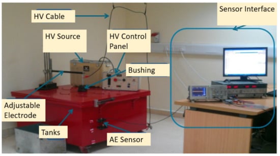
Figure 1.
Overall Experimental Setup.
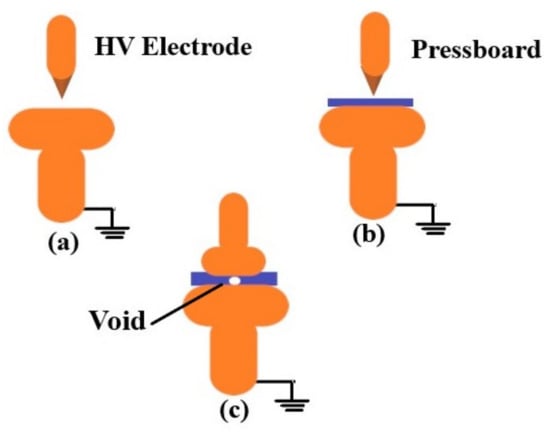
Figure 2.
Generated PD (a) sharp point to plane electrode (b) surface discharge (c) void discharge.
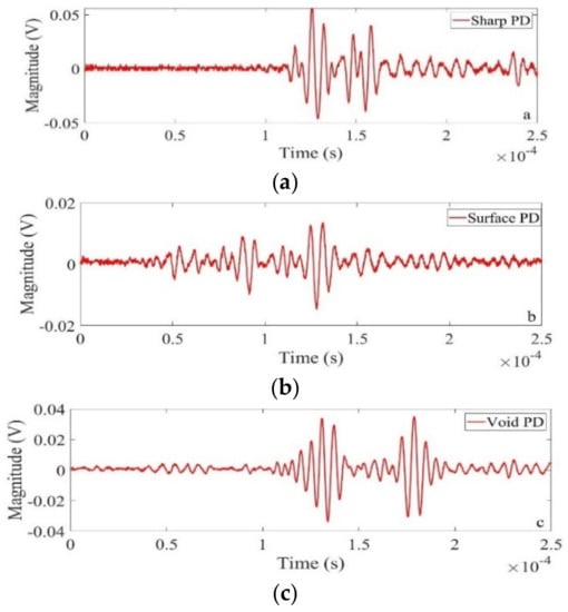
Figure 3.
Laboratory measured PD signals. (a) Sharp PD, (b) Surface PD, (c) Void PD.
The high voltage source is a 40 kV, 10 mA 50/60 Hz AC tester that is connected to an electrode system that could be adjusted to produce the desired PD type. An AE sensor connected with an oscilloscope at a sampling frequency of 10 M sample/sec for a window of 2500 samples interfaced with MATLAB is used for data acquisition. The oil-filled tank used here is of dimension 1 × 1 × 0.5 m. The AE sensor has a bandwidth of 100–450 kHz with a resonance frequency of 150 kHz. Silicone grease is applied between the surface of the tank and AE sensor to reduce the reflections.
2.1. PD Source Location
Figure 4 shows the top view of the tank where 9 holes are created in order to change the PD source location accordingly. The various PD forms are simulated in locations 4 and 9. Location “4” is 36 cm away from the AE sensor and location “9” is 95 cm away. The main objective of using 2 locations is to investigate the impact of training and testing at 2 different locations and to analyze the performance of the extracted features in classifying PD sources.
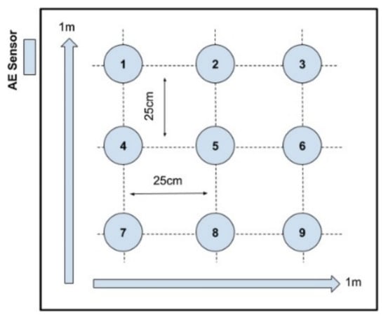
Figure 4.
PD location relative to AE sensor.
2.2. Oil Temperature
The temperature has a significant effect on the propagating velocity of the signal. Based on the loading condition, the transformer’s insulating oil temperature varies. This can affect the efficiency of the classifier as AE waves have different speeds at different oil temperature. Since there seems to be a limited maximum velocity at a low temperature where the oil was approaching the consistency of grease. As the temperature rises, the velocity drops off significantly. The relationship between oil temperature and acoustic wave speed is given in Table 1.

Table 1.
Speed of AE Waves in Oil at Different Oil Temperatures.
3. Extraction of Singular and Hyper Features
3.1. Singular Value Decomposition
Singular value decomposition is an orthogonal matrix transformation algorithm where the singular value has strong numerical stability when the matrix elements are shifted. A matrix [A] of rank R can be broken down into the product of three matrices with the SVD process. This method is usually represented as,
where and are orthogonal matrices; is a diagonal matrix. The diagonal matrix contains the square root of the eigen values of and represented as
These are called the singular values of the matrix [S] and ≥ SR ≥ 0. The rank of the matrix represents the number of independent hidden variables in the data.
The singular features have their advantages like the singular values represent each subspace’s energy distribution, which implies that the larger singular values contain more energy. Expressing a feature matrix in the form of singular values is conducive to compressing the scale of the feature vectors. In other words, if the feature matrix element is modified, there is no significant variation in its singular values.
3.2. Hankel Matrix-Based Singular Value Decomposition
Jiang had proposed Hankel SVD (HSVD) for bearing fault analysis [15]. Similar to their concept, this study also uses the Hankel matrix in SVD to extract the features. A Hankel matrix is a symmetric matrix that is built from the original time series. Let A be the measured acoustic PD signal. i.e., . The Hankel matrix of the input signal A can be obtained by sliding a window having a length of m over the corresponding vector and can be written as,
The Hankel matrix in Equation (4) is used in Equation (1) for singular value decomposition. The change in the order of the Hankel matrix can result in different decomposition results, and hence the SVD model could show more versatility as a feature extraction method in data classification.
3.3. Enhanced Singular Value Decomposition
The Enhanced SVD (ESVD) method proposed in [13] is used here to extract singular features. In the traditional SVD method, the data is decomposed into three matrices, and the dominant eigen values are selected as singular values. In the ESVD method, reconstruction is done similar to PCA. In Equation (1), V is the right singular vector that satisfies the equation, VVT = I. These right singular vectors are found to be sufficient for procuring the singular values. This reconstruction helps to capture the important components in the lowest index.
3.4. Enhanced Hankel Singular Value Decomposition
Instead of applying the ESVD to a normal matrix, in this paper, it will be applied to the Hankel matrix. The enhanced Hankel SVD (EHSVD) is used to generate the residual matrix by selecting a few singular vectors corresponding to the largest singular values.
3.5. Selection of Singular Features by Difference Spectrum
Singular features depict the characteristics of the signal and, hence, greatly influence the recognition rate of the classifier. In general, the singular values of a signal will be in the front, and the singular values of the noise will be uniformly distributed across the sequence. Here, the difference spectrum concept is proposed to select the effective singular values. The automatic selection of effective singular values can be realized by the peak of the difference spectrum. A signal corrupted with noise can be expressed as,
where x is the original signal, n is the noise signal, N is the length of the signal. After the signal arranged in Hankel matrix, we get matrix A as sum of two matrices.
where Ax and An are Hankel matrices created from x(i) and n(i), respectively. In a Hankel matrix, the next row lags the first row by only one data. According to [16], the two adjacent row vectors of the Hankel matrix created from signal s(i) will be highly correlated and the number of non-zero singular values will be just equal to the rank of the matrix. If the rank is K, then number of non-zero singular values will be equal to the rank K and rank is less than min (m, n). The singular vector of the signal can be written as . Whilst considering the noise, even though the next row trails by only one element of the first-row vector, there is no correlation between the data. Hence, the matrix is a full rank matrix, and the rank is .
The singular vector of noise can be written as, and its length is . Hence, in a Hankel matrix of the noisy signal, L-j values are less than first j values and to identify the sudden change in the jth singular value, the difference spectrum is introduced. The forward difference between the singular values is calculated by,
The sequence is called difference spectrum of singular value. When the difference in two adjacent singular values is high, a peak is generated in the difference spectrum, which implies that the maximum sudden shift in sequence occurs in the kth singular value. The singular value sequence obtained by HSVD and the calculated difference spectrum is given in Figure 5. The change in variation of singular feature is clearly visible in the plot. There are, totally, two peaks in the difference spectrum plot, and the highest peak is at the fourth coordinate, which shows that maximum sudden change in a singular value is happening at the coordinate. This represents the border between the signal and noise singular values.
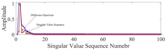
Figure 5.
HSVD singular value sequence and its difference spectrum.
Apart from the singular values, the structure of the Hankel matrix also greatly influences the signal processing results. The column of the H-Matrix is calculated using the formula (N + 1 − m), where m is number of rows and N denotes the number of samples (here N = 2500) and in a trial-and-error method m values are varied from 100 to 200 and the highest accuracy is achieved for m = 100.
3.6. Hypergraph Based Hyper Features
Hypergraph (HG) is a tool in the area of clustered data in the form of hyper-edges, which nicely exhibit the relation among features in terms of both geometry and topology mainly to reduce the computational burden of a chosen problem and, hence, it has been widely used for classification problems. Moreover, exploiting its properties to move towards their features called “hyper features” necessitate machine intelligence to be made inbuilt in any proposed technique [17].
HG can represent the binary relation between vertices representing data points to n-array relations by including more than two vertices in an edge called hyper-edge. Mathematically, hypergraph can be defined as, , where is the non-empty, finite set called vertices and is the non-empty subset of X called hyper-edges. In many data science applications, when we represent data points as vertices, we come across having pairwise relations, where an interesting and useful property (called Helly property) is observed. If all pairwise intersecting hyper-edges have a common intersection, then that hypergraph is said to obey Helly property. Consequently, there can be Helly (Figure 6a), Non-Helly (Figure 6b) and Isolated hyperedges (Figure 6c) can be observed once the represented in terms of hyper-edges constituting a Hypergraph. A machine learning algorithm learns Helly and Non-Helly and isolated hyper-edges from the incidence Matrices of the Hypergraph [18].
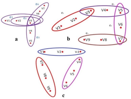
Figure 6.
Hypergraph representation of data: (a) intersecting hyper-edges with common intersection (Exploits Helly property), (b) pairwise intersecting hyper-edges without common intersection (Lack of Helly property) and (c) isolated hyper-edges.
3.6.1. Hypergraph Preliminaries
Every feature selection method mainly aims at a reduced number of features to achieve good classification accuracy when trained with any learning model. The error of the learning model increases due to the presence of redundant features. Hence, HG is introduced for the identification of optimal feature subset with minimal time complexity. The HG feature selection consists of two phases. In the first stage, hyper-edges of the HG are obtained by establishing topological and geometrical connections between the features. The hyper-edges and vertices correspond, respectively, to the data set samples and features [18]. In the second stage, Helly property of the HG is applied to the intersecting hyper-edges. In the further process, the features contained in the nonintersecting hyperedges are removed. The time complexity for identifying the ideal reduction is minimum because of HG’s Helly property. Even though the hypergraph can capture even small information, sometimes there is a possibility for redundant features. This is eliminated by using the Trim Hypergraph algorithm. After trimming, the Helly, Non-Helly and isolated hyperedges are taken for classification. This repetitive feature removal helps in reducing the computation time [19].
3.6.2. Selection of Hyper Features
The Helly property of HG helps in eliminating the redundant features in the data. Hyperedges are procured after applying the HG algorithm which helps in reducing the structure of the PD data (Table 2). The threshold is varied between 0.25 to 1.5 and we attained the best accuracy when the threshold to select isolated hyperedges was 1. Redundant hyperedges are eliminated using the HG’s trim property, as there may be an instance where these redundant hyperedges may be mistakenly predicted to apply to isolated hyperedges [18].
Table 2.
Hypergraph Representation of Data.
3.7. Fusion of Hankel Singular and Helly Hypergraph Features
The fusion of the two different groups of features obtained from the Hankel structure of PD data and hypergraph structure of PD data have been obtained using the following steps:
- Singular features have been derived from the Hankel structured data.
- Helly features have been extracted from HG representation of PD data as mentioned below.
- The feature vectors of PD data obeying the Helly property of HG have been considered first.
- The isolated and Non-Helly features of PD data have been obtained from the respective incidence matrices of the HG.
- The interdependencies of hyper features (Helly, Non-Helly and isolated) and the singular features have been found by using the rank minimization algorithm [20] by rearranging both the group of features once again in Hankel form.
- The interdependent Hyper features obtained from rank minimization algorithm of step 3 have been removed by trim hypergraph property.
The rank minimized Hankel-Hyper features thus provide the fused features which caused the higher recognition rate. Extraction of singular features and hyper features from the measured PD signal is given in Figure 7.
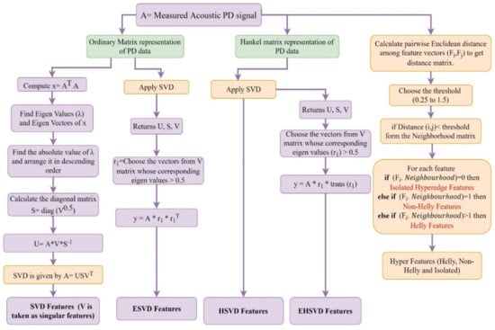
Figure 7.
Flowchart of singular feature and hyper feature extraction from acoustic PD signals.
The metric accuracy is used to quantify the performance of classifiers. Accuracy () is the ratio between correct observation and total observations defined in Equation (8):
where TP, TN, FP and FN are the true positives, true negatives, false positives and false negatives, respectively, in the confusion matrix.
4. Results and Discussion
In this work, singular features, along with hyperparameters, are used to discern between different PD types. A total of three different types of PD are considered; namely, sharp, void and surface discharges. The simulations are conducted using Python programming language running in Intel(R) Core i5-7300HQ processor with 2.50 GHz clock frequency and 8 GB RAM. The acoustic PD datasets captured from the experiments consists of 432 samples for each PD type. The main objective of this study is to examine the recognition rate with different measurement conditions. PD data is processed using different combinations of feature extraction techniques and classifiers. It is a multi-class classification problem. Training and testing data were acquired following a stratified shuffle split. In a total 855 samples (70% samples were taken for training, 10% for testing and 20% were taken for validation in each case study. All samples do exhibit insulation defects (one of the three defects mentioned earlier). Moreover, the imbalance in the data is measured for which we used the metric Imbalance Ratio (IR) to normalize the imbalanced data to the extent of balancing them to run the algorithm. IR is defined as:
is the sample size of the largest majority class and is the sample size of the smallest minority class.
4.1. Case Study-I: PD Type Classification at Different PD Locations
In the first case study, PD experiments targeted the PD source location with respect to the AE sensors are considered. At first classification performance of individual location (location 9) is considered and the results are given in Table 3. The singular values are calculated from each sub-matrix arranged in the form of a vector and used to train the classifiers. The performance of the four different singular features is evaluated with and without hyper features.
Table 3.
Case Study-I: Singular Feature Performance with and Without Hyper Parameters (for Different PD Location).
It is evident from Table 3 that HSVD features along with HG attained the highest accuracy using all classifiers. Moreover, RF and KNN showed the highest classification accuracy in all cases. Additionally, using HG resulted in a significant increase in the classification accuracy with all classifiers. This could be attributed to the fact that hypergraph representations allowed hyperedges to be linked in vertices and, hence, they can capture relationships between features.
The performance of the proposed feature extraction method is also compared to the results of features extracted by principal component analysis, wavelet, discrete Fourier transform (as given in [14]), EEMD and FD based extraction method and its results are tabulated in Table 4. The accuracy shows the superiority of the singular-hyper feature combination in classifying the PD sources. The extracted HSVD-HG features attained the highest accuracy of 97.8% in classifying PD sources measured at location 9 using KNN as a classifier.
Table 4.
Case Study-I: Singular-Hyper Feature Performance-Comparison with [14] (for Different PD Location).
The effectiveness of the features with different training and testing samples is also addressed. Here, PD data is trained with location 4 samples and tested with location 9 samples. In the previous work reported in the literature [14], the highest achieved accuracy was 65% using wavelet features with KNN as the classifier and 85% of accuracy was reported when using short time Fourier transform features with convolutional neural network as classifier [21]. The reason for the low accuracy was attributed to the fact that as the signals captured from PD location 9 suffered from additive attenuation; hence, these signals will be more prone to noise. Since the proposed singular-hypergraph feature combination can classify the PD sources in high noisy condition, it is expected to classify attenuated PD signals that might be corrupted with noise. The classification accuracy is given in Table 5.
Table 5.
Case Study-I: Classifiers Performance when Training and Testing with Different Samples.
It is evident that the highest attained classification accuracy is 94.1% with the HSVD-HG feature combination. This relatively high accuracy outperforms previously reported research where the maximum attained classification accuracy was 85%. One of the major restrictions to expand the application of machine learning in PD classification is the necessity to train the data at a large number of scenarios. However, being able to test the data at a condition that has never been used in the classifier training process is significant and can help to further apply this approach in the field.
4.2. Case Study-II: Classification of PD Sources for Input Data Trained and Tested under Different Oil Temperature
In the case study-II, PD data measured at a single location, but at different oil temperatures are considered. Two types of PDs are investigated here: surface and void PDs. 432 samples are considered per PD type with about 70% used for training and 30% for testing. As told in the previous case study, the recognition rate of the algorithm is tested for two conditions.
In practice, the recognition rate of the classifier reduces when a system is trained and tested with different conditions. Table 6 shows the recognition rate of the classifier when training and testing are done with different data (training at 23 °C and testing at 70 °C) and Table 7 shows the classifier performance of case study-II (training at 70 °C and testing at 23 °C). The performance of ESVD-HG attains lower accuracy since it cannot capture the non-linearity in the dataset. The performance of the EHSVD-HG is better than ESVD-HG in this case study. The Hankel structure helps in enhancing the recognition rate here. From the results, it is evident that the recognition rate of HSVD-HG features outperforms other feature combinations for all the classifiers. It is interesting to see the good performance of RF with all the combination of features. Compared with the previous work reported in literature [4], the RF classifier attained higher accuracy of 100% data (training at 23 °C and testing at 70 °C and for vice versa condition). This ensures our previous observations in case study-I, that the recognition rate of HSVD-HG is better compared with other feature extraction methods.
Table 6.
Case Study-II: Classifiers Performance when Training and Testing with Different Oil Temperatures (training at 23 °C and testing at 70 °C).
Table 7.
Case Study-II: Classifiers Performance when Training and Testing with Different Oil Temperatures (training at 70 °C and testing at 23 °C).
4.3. Case Study-III: PD Classification under Noisy Condition
The previous results showed that the proposed features could classify the PD sources with higher accuracy compared to previous research [14]. The results also suggested that under noise-free condition, the extracted singular and hypergraph features performed better when they are combined. Therefore, when investigating the performance of the classification accuracy under noisy conditions, the combination of singular-hypergraph features is taken into account.
The major three types of noise that couples with PD are discrete spectral interference, pulse shaped interference and white noise and random noise. The sources of these noise are clearly explained in [20,22]. To mimic the real noise environment, a dc motor is used at different speed to generate different levels of noise. The motor is placed 5 cm away from the transformer tank on the ground. The classifiers are tested with noisy PD data that are not used for training. The tests are repeated on an average of 20 times and the classification accuracy is given in Table 8.
Table 8.
Case Study-III: Classifiers Performance on Noisy PD Data.
It is evident that there is decrease in the accuracy of the classifiers compared to previous case studies. However, the rate of decrease is not same, since each feature combination and classifier has its own noise tolerance. The classification accuracy of HSVD-HG is high compare to other feature extraction methods. The recognition accuracy of ESVD-HG and EHSVD-HG is not more than 87%. This poor performance is due to the problem in the reconstruction and in the selection of singular values. Similar to the noise-free cases, the performance of the HSVD-HG outperforms all other feature extraction methods. The classification accuracy of HSVD-HG feature extraction for different noise levels and for different classifiers is given in Figure 8. It is evident from Table 7 that other feature extractions methods are not consistent, as, in some cases, they provide high classification accuracy and in others, the classification accuracy is extremely low.
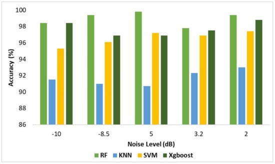
Figure 8.
Accuracy comparison plot for different noise level for HSVD-HG features.
4.4. Influence of Hyperparameter
The Structure of the Hankel matrix and the selection of the hyper feature plays the major role in achieving higher accuracy. The choice of window length (m) and the number of singular values selected influence the classification results, since choosing improper values will lead to misinterpretation. The variations in “m” may influence the closeness in the singular values. Figure 9 shows the variations in classification accuracy for different values of m. The m values are varied between 20 to 250. The highest accuracy is achieved for m = 100. The number of singular values is selected by the difference spectrum concept and it is explained in Section 3.5 [23]. In the selection of hyper features, the threshold places the major role. The threshold is varied between 0.25 to 1.5 in calculating pairwise distance among the features by Euclidean distance method. The variations in the accuracy for different threshold value is given in Figure 10. The highest accuracy is achieved when threshold is set to 1 for hyperedges selection. Table 9 below shows how hyper parameter tuning can improve the classification accuracy. Before tuning the classification accuracy of case study-I is 96.8%. After hyper parameter tuning the classification accuracy increased to 99.2%.
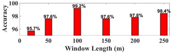
Figure 9.
Accuracy comparison plot for various values of ‘m’.
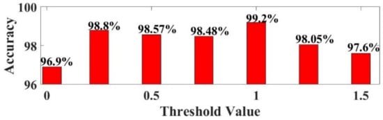
Figure 10.
Accuracy comparison plot for different threshold value.
Table 9.
Classification accuracy before and after hyper parameter Tuning.
4.5. The Complexity Analysis
The complexity of the proposed algorithm is dependent on two levels of the model: (1) Singular feature extraction, (2) Hyper features extraction.
4.5.1. Singular Feature
Starting from SVD till EHSVD, we only use Matrix structures. The complexity is proven to be , where are constants. Therefore, it can be represented by its highest component bounded above by , where n is the order of the Hankel Matrix.
4.5.2. Hyper Feature
The hyper features are obtained through HG representation of the data through hyperedges. The related features (points) are represented as a vector quantity. The related hyperedges are captured through incidence matrices of the Hypergraphs. The Helly hyperedges (vectors) generation leaves a complexity of , n-vertices and m-hyperedges and it is bounded above by . Hence, complexity of the algorithm turns out to be . Since the occurrence of PD events are random, the algorithm is expected to be of exponential complexity. As we infer that both Helly Hypergraph and SVD have polynomial complexity, we started hybridizing them. The algorithm is found to be convergent for all sample data and we have ascertained complexity through recalculations.
5. Conclusions
In this paper, feature extraction methods based on singular features (SVD, HSVD, ESVD and EHSVD) and hypergraph features are proposed for partial discharge feature extraction. Artificial defects are created in the lab and AE sensor is used to measure the PD signals. The experiments provided insight into understanding the characteristics of AE sensor signals. Among all the four cases, classification accuracy achieved by HSVD-HG combination features is notably high compared to the other features.
First, the algorithm is tested for different measurement locations. The proposed feature extraction method recognition rate is high even though the classifier trained and tested with different data. The algorithm’s recognition rate efficacy is also tested for PD measurement at different temperature conditions. The results showed that the HSVD-HG combination classified the PD with higher recognition rate.
The proposed feature extraction method is impervious to noise addition, which hinders the use of noise elimination schemes during classification. Overall, developments based on these findings are expected to be developed and tested for the design of automated power transformer monitoring systems in the future. Moreover, this proposed algorithm could be implemented to separate multiple PD sources by integrating Stockwell transform with Hankel transform.
Author Contributions
Conceptualization, S.G. and J.S.; methodology, S.G. and K.K.; software, V.R.; validation, A.E.-H. and S.G.; formal analysis, S.G. and J.S.; investigation, A.E.-H. and S.G.; resources, A.E.-H.; data curation, A.E.-H.; writing—original draft preparation, S.G.; writing—review and editing, S.G., A.E.-H. and K.K.; visualization, J.S. and A.E.-H.; supervision, A.E.-H.; project administration, A.E.-H.; funding acquisition, N/A. All authors have read and agreed to the published version of the manuscript.
Funding
This research received no external funding.
Institutional Review Board Statement
Not applicable.
Informed Consent Statement
Not applicable.
Data Availability Statement
Not applicable.
Acknowledgments
The authors thank the Management of SASTRA University and Tata Realty-IT City- SASTRA Srinivasa Ramanujan Research cell.
Conflicts of Interest
The authors declare no conflict of interest.
References
- Kuo, C.C.; Shieh, H.L. Artificial classification system of aging period based on insulation status of transformers. In Proceedings of the 2009 International Conference on Machine Learning and Cybernetics, Baoding, China, 12–15 July 2009; Volume 6, pp. 3310–3315. [Google Scholar]
- Kreuger, F.H.; Gulski, E.; Krivda, A. Classification of Partial Discharges. IEEE Trans. Electr. Insul. 1993, 28, 917–931. [Google Scholar] [CrossRef]
- Hikita, M.; Okabe, S.; Murase, H.; Okubo, H. Cross-equipment evaluation of partial discharge measurement and diagnosis techniques in electric power apparatus for transmission and distribution. IEEE Trans. Dielectr. Electr. Insul. 2008, 15, 505–518. [Google Scholar] [CrossRef]
- Woon, W.L.; El-Hag, A.; Harbaji, M. Machine learning techniques for robust classification of partial discharges in oil-paper insulation systems. IET Sci. Meas. Technol. 2016, 10, 221–227. [Google Scholar] [CrossRef]
- Raymond, W.J.K.; Illias, H.A.; Bakar, A.H.A.; Mokhlis, H. Partial discharge classifications: Review of recent progress. Meas. J. Int. Meas. Confed. 2015, 68, 164–181. [Google Scholar] [CrossRef]
- Dey, D.; Chatterjee, B.; Chakravorti, S.; Munshi, S. Cross-wavelet transform as a new paradigm for feature extraction from noisy partial discharge pulses. IEEE Trans. Dielectr. Electr. Insul. 2010, 17, 157–166. [Google Scholar] [CrossRef]
- Wu, M.; Cao, H.; Cao, J.; Nguyen, H.L.; Gomes, J.B.; Krishnaswamy, S.P. An overview of state-of-the-art partial discharge analysis techniques for condition monitoring. IEEE Electr. Insul. Mag. 2015, 31, 22–35. [Google Scholar] [CrossRef]
- Evagorou, D.; Kyprianou, A.; Lewin, P.L.; Stavrou, A.; Efthymiou, V.; Metaxas, A.C.; Georghiou, G.E. Feature extraction of partial discharge signals using the wavelet packet transform and classification with a probabilistic neural network. IET Sci. Meas. Technol. 2010, 4, 177–192. [Google Scholar] [CrossRef]
- Dai, D.; Wang, X.; Long, J.; Tian, M.; Zhu, G.; Zhang, J. Feature extraction of GIS partial discharge signal based on S-transform and singular value decomposition. IET Sci. Meas. Technol. 2017, 11, 186–193. [Google Scholar] [CrossRef]
- Sahoo, N.C.; Salama, M.M.A.; Bartnikas, R. Trends in partial discharge pattern classification: A survey. IEEE Trans. Dielectr. Electr. Insul. 2005, 12, 248–264. [Google Scholar] [CrossRef]
- Raymond, W.J.K.; Illias, H.A.; Bakar, A.H.A. High noise tolerance feature extraction for partial discharge classification in XLPE cable joints. IEEE Trans. Dielectr. Electr. Insul. 2017, 24, 66–74. [Google Scholar] [CrossRef]
- Xia, Y.; Zhou, W.; Li, C.; Yuan, Q.; Geng, S. Seizure detection approach using S-transform and singular value decomposition. Epilepsy Behav. 2015, 52, 187–193. [Google Scholar] [CrossRef] [PubMed]
- Mandal, S.; Santhi, B.; Sridhar, S.; Vinolia, K.; Swaminathan, P. Sensor fault detection in Nuclear Power Plant using statistical methods. Nucl. Eng. Des. 2017, 324, 103–110. [Google Scholar] [CrossRef]
- Harbaji, M.; Shaban, K.; El-Hag, A. Classification of common partial discharge types in oil-paper insulation system using acoustic signals. IEEE Trans. Dielectr. Electr. Insul. 2015, 22, 1674–1683. [Google Scholar] [CrossRef]
- Jiang, H.; Chen, J.; Dong, G.; Liu, T.; Chen, G. Study on Hankel matrix-based SVD and its application in rolling element bearing fault diagnosis. Mech. Syst. Signal Process. 2015, 52–53, 338–359. [Google Scholar] [CrossRef]
- Zhao, X.; Ye, B. Selection of effective singular values using difference spectrum and its application to fault diagnosis of headstock. Mech. Syst. Signal Process. 2011, 25, 1617–1631. [Google Scholar] [CrossRef]
- Raman, M.R.G.; Somu, N.; Kirthivasan, K.; Sriram, V.S.S. A Hypergraph and Arithmetic Residue-based Probabilistic Neural Network for classification in Intrusion Detection Systems. Neural Netw. 2017, 92, 89–97. [Google Scholar] [CrossRef] [PubMed]
- Suganya, G.; Ardila-Rey, J.A.; Krithivasan, K.; Subbaiah, J.; Sannidhi, N.; Balasubramanian, M. Development of Hypergraph Based Improved Random Forest Algorithm for Partial Discharge Pattern Classification. IEEE Access 2021, 9, 96–109. [Google Scholar] [CrossRef]
- Krithivasan, K.; Pravinraj, S.; Shankar Sriram, V.S. Detection of Cyberattacks in Industrial Control systems using Enhanced Principal Component Analysis and Hypergraph based Convolution Neural Network (EPCA-HG-CNN). IEEE Trans. Ind. Appl. 2020, 56, 4394–4404. [Google Scholar] [CrossRef]
- Suganya, G.; Subbaiah, J.; Cavallini, A.; Krithivasan, K.; Jayakumar, J. Development of Hankel-SVD hybrid technique for multiple noise removal from PD signature. IET Sci. Meas. Technol. 2019, 13, 1075–1084. [Google Scholar] [CrossRef]
- Woon, W.L.; Aung, Z.; El-Hag, A. Intelligent monitoring of transformer insulation using convolutional neural networks. In Lecture Notes in Computer Science (Including Subseries Lecture Notes in Artificial Intelligence and Lecture Notes in Bioinformatics); Springer: Cham, Switzerland, 2018; Volume 11325, pp. 127–136. [Google Scholar]
- Hussein, R.; Shaban, K.B.; El-Hag, A.H. Robust Feature Extraction and Classification of Acoustic Partial Discharge Signals Corrupted With Noise. IEEE Trans. Instrum. Meas. 2017, 66, 405–413. [Google Scholar] [CrossRef]
- Mahmoudvand, R.; Zokaei, M. On the singular values of the Hankel matrix with application in singular spectrum analysis. Chil. J. Stat. 2012, 3, 43–56. [Google Scholar]


Publisher’s Note: MDPI stays neutral with regard to jurisdictional claims in published maps and institutional affiliations. |
© 2021 by the authors. Licensee MDPI, Basel, Switzerland. This article is an open access article distributed under the terms and conditions of the Creative Commons Attribution (CC BY) license (http://creativecommons.org/licenses/by/4.0/).