Abstract
This paper contains studies of daily energy production forecasting methods for photovoltaic solar panels (PV panel) by using mathematical methods and fuzzy logic models. Mathematical models are based on analytic equations that bind PV panel power with temperature and solar radiation. In models based on fuzzy logic, we use Adaptive-network-based Fuzzy Inference Systems (ANFIS) and the zero-order Takagi-Sugeno model (TS) with specially selected linear and non-linear membership functions. The use of mentioned membership functions causes that the TS system is equivalent to a polynomial and its properties can be compared to other analytical models of PV panels found in the literature. The developed models are based on data from a real system. The accuracy of developed prognostic models is compared, and a prototype software implementing the best-performing models is presented. The software is written for a generic programmable logic controller (PLC) compliant to the IEC 61131-3 standard.
1. Introduction
The basis for being on the electricity market is forecasting generation and demand for electricity. Power generators and distributors use short-term forecasting most often. The main problem of energy producers are external factors that affect the production level; in other words, weather conditions [1,2]. In case of producers that sell energy on energy exchanges, the use of a forecast with a high error may result in financial losses. The reason for these losses is an inappropriate evaluation of energy supply and presenting an offer with a price significantly deviated from the market price. However, accurate forecasts reduce costs and increase profits, thanks to improving the efficiency of the procurement process and energy distribution [3,4]. The choice of prognostic methods may depend on the scope of information. There are many forecasting methods, and some of them are used in power engineering.
Generally, the methods of power forecasting in solar systems can be divided into physical, statistical, artificial intelligence and others. Some statistical methods in prediction can be found in [2,5]. The comparison of the physical model with the multilayer perceptron neural network (MLP NN) model for power predictions is presented in [6]. Among others artificial intelligence methods, MLP neural networks [1,2,6,7], radial basis function neural networks (RBF NN) [8], physical hybrid artificial neural networks [9], recurrent neural networks [8] and deep neural networks [10] are used to predict the power and energy of photovoltaic sources.
A large part of the developed methods has some disadvantages, such as a relatively large average accuracy error and the dependence of a specific photovoltaic system design on the geographical location. In order to increase quality of forecasting power, some authors have developed hybrid models [11,12] and applied various methods of optimization of model parameters calculation [13] or used methods for input data imputation [14]. Implementation of the mentioned methods requires devices with high computing power and the use of specialized software libraries. This may lead to the limitation of technology to the area of computing centers and a lack of possibility to deploy the technology on platforms commonly used in the industry, such as programmable logic controller (PLC) devices.
The goal of the paper is to evaluate fuzzy logic-based analytical models applied to forecast daily energy generation by an installation of PV panels and compare these models to an ANFIS system and to analytical models taken from the literature. The purpose of the research is the following. The market forces green energy producers to have models for energy production forecasting. In order to improve the accuracy of these models, local climate conditions should be taken into account. The existence of these conditions has impact on the precision of models. Having set up a PV panel site, it is recommended to conduct measurements in order to obtain data required for building a model of the site. Several examples of fuzzy logic applications in power engineering are control of a battery energy storage system [15], energy management in a DC microgrid [16], design of a voltage source inverter [17] and control of grid-connected inverters [18]. Experience from these areas points to the fact that the quality of fuzzy logic-based models is better or comparable to systems designed by applying other methods. An advantage of fuzzy models is their rule-based form, which is easy to understand for a human. However, this implies that in order to examine properties of the system, oftentimes, simulations must be performed because of absence of analytical methods. Model-free and heuristic design methods, deficit in analytical tools, can be a reason that the fuzzy logic is not preferred solution in a given domain [19]. Authors of this paper focused on models that are based on the zero-order Takagi-Sugeno fuzzy inference system with special kinds of fuzzy sets, as described in the thesis [20]. This approach allows to express fuzzy rules as polynomials, compare models designed as a set of fuzzy rules with mathematical models and utilize analytical methods to examine features of the system. A practical application of the theory described previously [20] is presented in [21,22] for an attitude control system and a mechanical vibration limiting system. In one paper [23], it was shown that fuzzy models obtained by the use of methods from [20] can be efficiently implemented in hardware field-programmable gate array devices (FPGA).
The novelty of this work is an application of analytical methods in fuzzy modeling from [20] in the area of power engineering. The paper shows that using the presented techniques, we can obtain a high-quality fuzzy logic-based model for predicting daily energy production by a PV panel. Because the model is identical with a polynomial function, its characteristics can be studied with the use of formal methods.
We also show an exemplary implementation of our achievements. Commercial products utilizing fuzzy logic are considered to be innovative. The result of our research can be a base to develop a novel device that can be deployed as a data processing node at the layer 2 in the edge computing architecture of a Smart Energy System [24]. The hardware platform for the device can be a standard general-purpose PLC unit. The program, which implements fuzzy logic systems, neither requires high computing power nor non-standard software components.
2. Methods for Predicting the Power and Energy of Photovoltaic Panels
2.1. Description of the PV System
The research was carried out on the basis of a photovoltaic panel system. The PV system is composed of three modules (monocrystalline type), connected to the Soladin 600 solar inverter. Photovoltaic panels are positioned at 30 degrees to the horizon and are directed to the South. The total installation power is 330 [Wp]. The PV system works in Rzeszów (geographical location 50°02′ N 22°17′ E).
The photovoltaic measurement system included measurement of voltage and DC current in front of the inverter, voltage, AC current, power and frequency at the inverter output. At the same time, measurements of solar radiation in the plane of PV panels were made using a pyranometer. All parameters were measured on a current basis; however, their average values were recorded every minute in the database. The measurement data taken in the time interval from November to October of the next year were used for the research.
In our research, two measured factors were used in the PV system: the daily value of insolation and the total value of DC energy generated during the day, calculated per 1 [m2] of the active area of photovoltaic panels. In addition, measurements of the daily maximum temperature in the analyzed period came from a meteorological station in the system’s work place. Therefore, the forecasts of the daily energy produced in a PV system will be generated on the basis of two factors, i.e., air temperature and daily insolation. Developed forecasting models generate forecasts in the perspective of one day.
The total set of measurement data consisting of 347 samples (days) was divided into a training set (174 samples) and a test set (173 samples). This manner of division allowed to achieve even coverage of the measurement space with test and learning points. The algorithm for creating the learning set was as follows:
Let MST = (mST1, mST2, …, mSTn) be a sequence of measurements ordered by ascending temperature: mSTi is a tuple <t, g>, where t is the value of temperature and g is the value of insolation; ∀i = 1, 2, …, n − 1: mSTi·t ≤ mSTi + 1·t ∧ mSTi·g ≤ mSTi + 1·g.
Let MSG = (mSG1, mSG2, mSGn) be a sequence similar to the mentioned before, but ordered by ascending insolation: ∀i = 1, 2, …, n: mSGi·g ≤ mSGi + 1·g.
The learning set is defined as ML = MLT ∪ MLG, where MLT and MLG are given by (1) and (2):
MLT = {mSTi ∈ MST|∀i = 1, 2, …, n − 1: mSTi·t ≠ mSTi + 1·t},
MLG = {mSGi ∈ MSG|∀i = 1, 2, …, n − 1: INT(mSGi·g/50) ≠ INT(mSGi + 1·g/50)}.
The test set is defined as MT = MST/ML.
Based on the training set the parameters of the forecasting models were determined and the test set was used to verify these models.
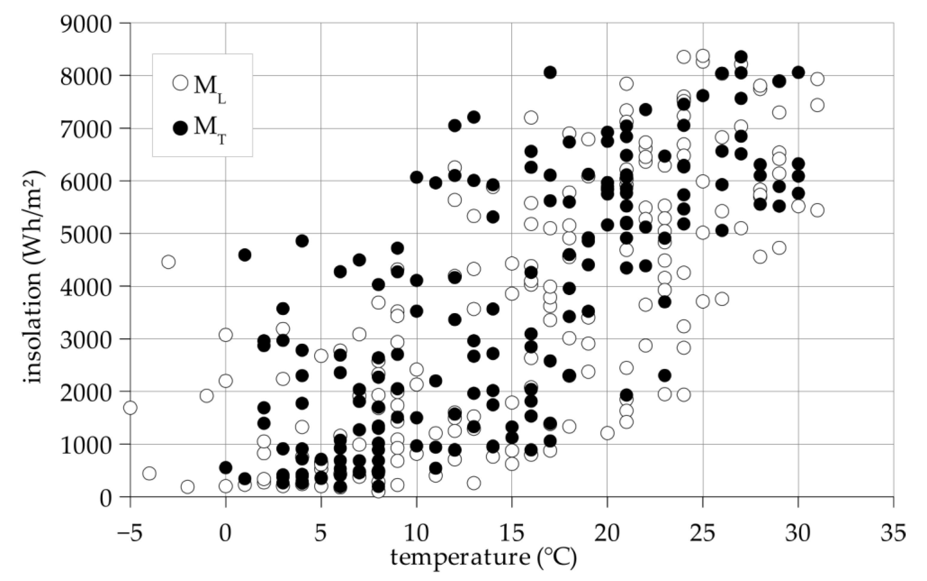
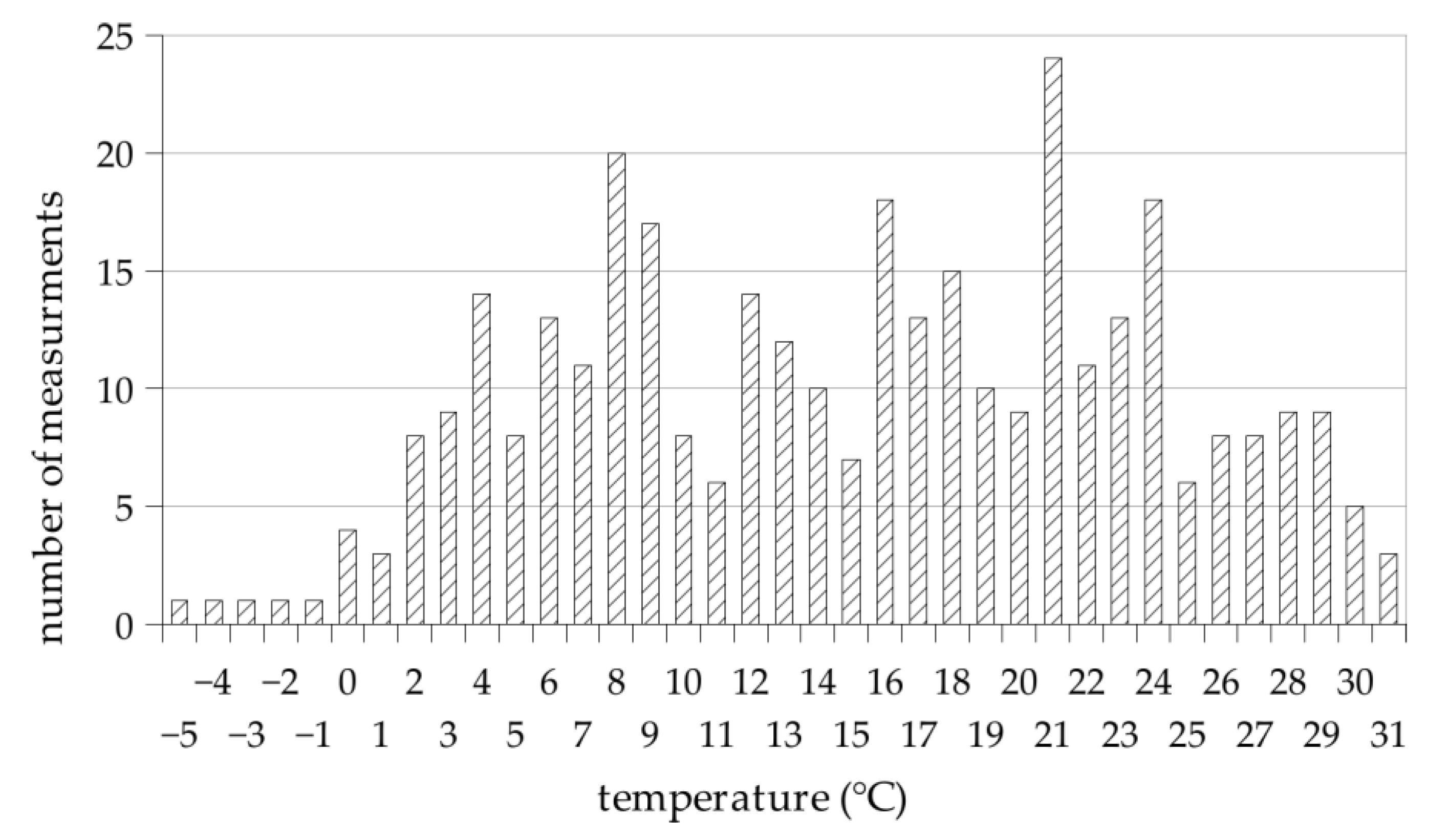
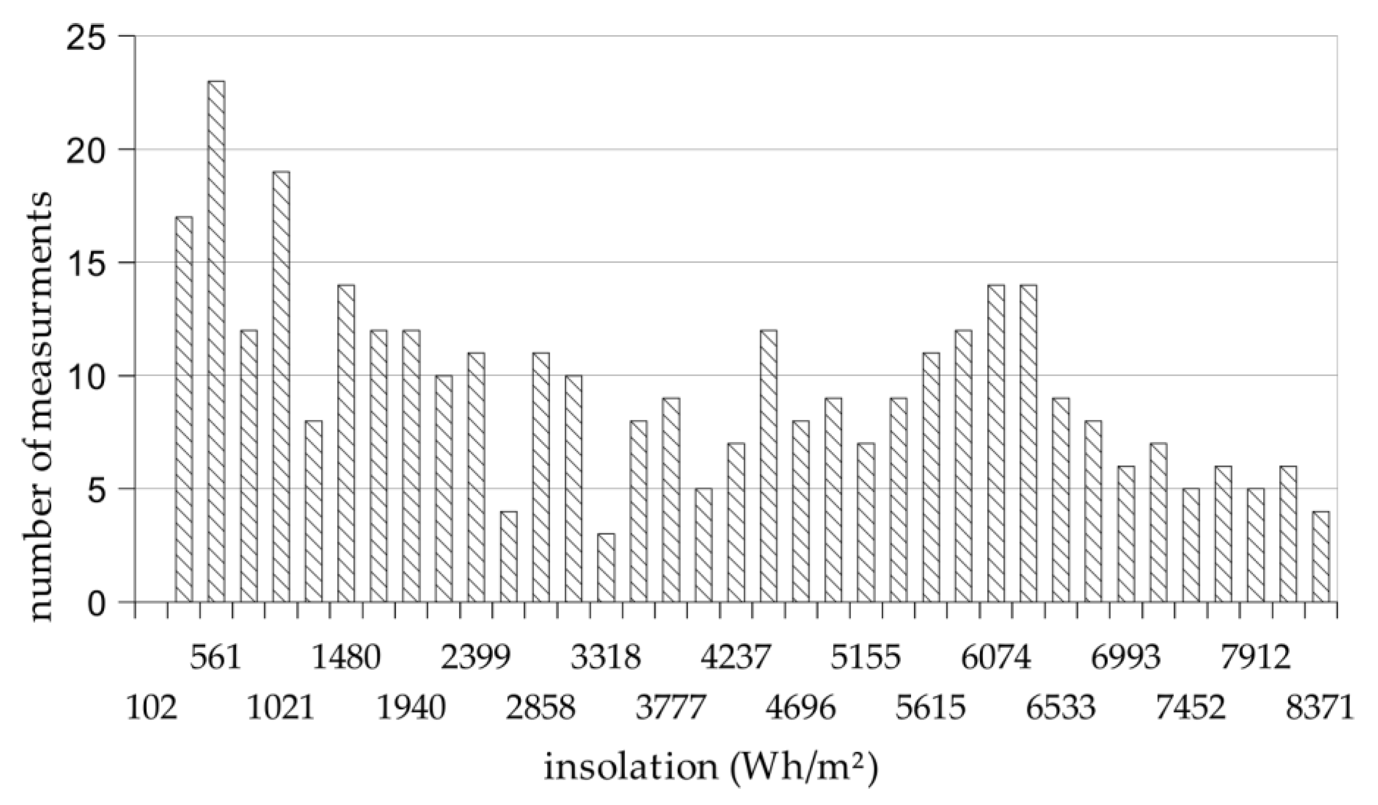
Figure 1 presents the distribution of measure points in space of air temperature (T) and insolation (G). Figure 2 presents the distribution of measurements in the air temperature set (T) and Figure 3 shows the distribution of measurements in the set of daily insolation (G).

Figure 1.
Distribution of measurement points (MT—test, ML—learning) in the space of temperature T and insolation G, T × G.

Figure 2.
Distribution of measurement points in the temperature set T.
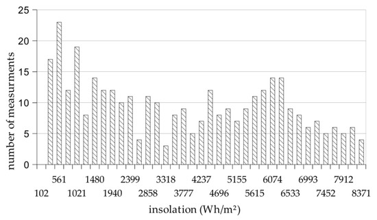
Figure 3.
Distribution of measurement points for the set of insolation G.
Figure 1, Figure 2 and Figure 3 allow to visually evaluate the quality of input data. From Figure 1, we can say that elements of learning and test sets are distributed quite uniformly over the space of measurements. Two remaining charts show values of temperature and insolation typical for the temperate climate area where the city of Rzeszów lies. Short winder days, cloudy spring and autumn are the reason for many measurements with low values of insolation and values of temperature around 8 °C.
2.2. Mathematical Modes of the Power Production of Photovoltaic Panels
In the literature [25,26], several models of estimation of daily power production by a solar panel operating in Maximum power point tracking (MPPT) conditions are presented. One paper [25] proposes the equation:
where: a′, b′, c′ and d′ are constants. Another model for determining the power of a PV panel is presented by the following formula [26]:
where G is the insolation in the plane of the PV panel, Gn is the insolation on the surface of the Earth in the horizontal plane, G0 is the standard insolation 1000 (Wh/m2), T is the air temperature, Tj is the temperature of the PV panel, Tjref is the reference temperature of the PV panel and Tjref = 25 (°C), AM is the air mass ratio, AM0 is the air mass ratio for the Sun at the zenith, AM0 = 1.5, A is the active surface of the panel and p, q, m and u are constants.
The following dependence allows replacing the solar insolation Gn with solar radiation G. We consider the average daily parameter measurements and assume that AM has a constant value for one daily measurement, depending on the calendar day. Because the G values are measured, the daily change of the AM parameter is included in the G measurement. With these assumptions, (2) takes the form:
where c′1, c′2, c′3, c′4 and c′5 are constants.
In [18], the value of c’5 ∈ (1.0618, 1.6601) was determined, depending on the panel manufacturer. In Equations (3)–(5), there is the parameter Tj—the panel temperature. The authors made air temperature measurements. In [27], it was shown that there is the following relationship between the air temperature and the panel temperature:
where h is a constant and t is the air temperature. Considering the above, Equation (3) takes the form:
and (5) can be simplified to the following formula:
where: a, b, c, d and e and c1, c2, c3, c4, c5 and c6 are constants.
Tj = t + h·G,
Pmax1 = a·G2 + b·G·t + c·G + d·t + e
Pmax2 = c1·G3+ c2·G2 + c3·G2·t + c4·t + c5·G + c6,
A higher degree of polynomial approximating power in relation to (5) results from the fact that (8) takes into account the dependence of photovoltaic panel efficiency on insolation. This phenomenon was not modeled in (5).
The measurements contain the total energy produced by one square meter of the PV panel surface during the period of 24 h, e.g., E = P × t, where P is the power of the PV panel operating under the MPPT condition, time t = const = 24 h.
Taking the above into account, we obtain energy E = k×P. If we use Matlab to find the constant coefficients of the polynomial equation of the power output of a PV panel, we have:
E = k·P = k·(c1·G3+ c2·G2+ c3·G2·t+ c4·t + c5·G + c6).
The value of the constant k will be included in the calculated coefficients c1, …, c6. The presented analysis allows to use measured energy E instead of power in the process of calculation constants c1, …, c6.
In order to interpolate the measurement results with (7) and (8), the following parameters were determined: a, b, c, d, e, c1, …, c6, h using Matlab’s lsqcurvefit function [28]. The interpolation method with minimization of mean square error was applied, as shown in Algorithm 1. Table 1 and Table 2 contain the calculated values of parameters.
| Algorithm 1 A Matlab program for computing coefficients of the Equation (5). | |
| 1: | fileID = fopen(’measurements.csv’,’r’); |
| 2: | formatSpec = ’%d %f %f’; sizeA = [3 Inf]; |
| 3: | test = fscanf(fileID,formatSpec,sizeA); test = test’; |
| 4: | fclose(fileID); |
| 5: | x1 = test(:,1); x2 = test(:,2); y = test(:,3); x = [x1 x2]; |
| 6: | p = [1, 1, 1, 1, 1]; |
| 7: | f = @(p,x) p(1) * x(:,2).^2 + p(2).*x(:,1).*x(:,2) + ... |
| 8: | p(3) * x(:,2) + p(4) * x(:,1) + p(5); |
| 9: | abcde = lsqcurvefit(f,p,x,y) |

Table 1.
Values of the parameters of Equation (7), calculated from the training data set.

Table 2.
Values of the parameters of Equation (8), calculated from the training data set.
2.3. Adaptive Network-Based Fuzzy Inference System ANFIS
In this section, the goal is to design a fuzzy application system that predicts the total daily production of electricity by the solar panel, based on insolation and air temperature.
The structure of the forecasting system was obtained using a classic engineering approach. The optimal values of the fuzzy system parameters were determined by Matlab software. The components of the system are presented in Figure 4.
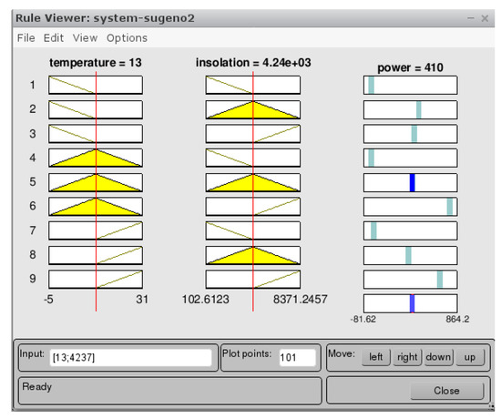
Figure 4.
The draft rule system based on ANFIS.
Based on the models presented in Section 2.2 and in accordance with the principles given in [29], let us introduce the following linguistic variables: temperature t, insolation g and power P. Let us define the following sets of linguistic values for the introduced variables:
t ∈ {low, medium, high},
g ∈ {low, medium, high},
P ∈ {low1, low4, low7, medium2, medium3, medium5, medium8, high6, high9}.
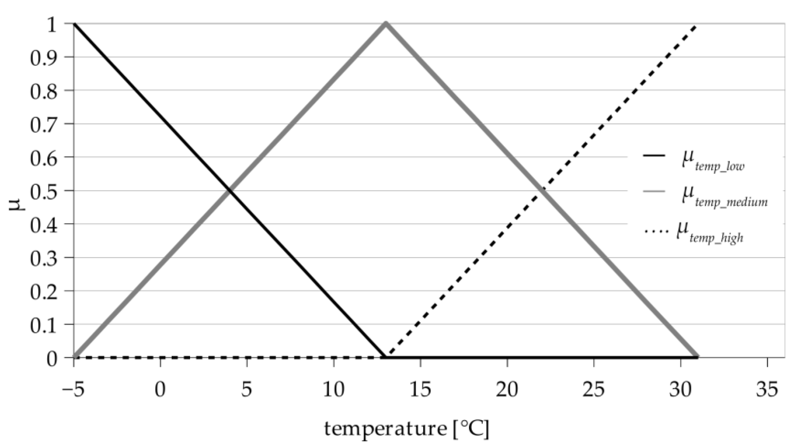
For the given values of the linguistic variables, we specify the triangular fuzzy sets, as shown in Figure 4. We do not specify sets for the variable P, because they will be determined automatically. Membership functions for the linguistic values are given by the following equations (where the symbols ∧ and ∨ mean the minimum and maximum, respectively):
and
Numerical constants that appear in (13) and (14) are taken from the measurements data and depend on minimal and maximal values of temperature and insolation. Ranges for t and g are as follows: t ∈ (−5; 31), g ∈ (102.6; 8371). Figure 5 shows the chart of functions given by (13); the chart of functions (14) looks similar.
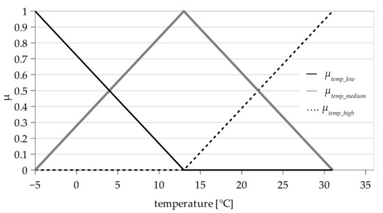
Figure 5.
The chart of membership functions of Equation (13).
Taking into account the power models from Section 2.2 and the values of variables t and g, nine rules can be formulated to determine the power produced by the panel.
| P | Temperature t | |||
| Low | Medium | High | ||
| insolation g | low | low1 | low4 | low7 |
| medium | medium2 | medium5 | medium8 | |
| high | medium3 | high6 | high9 | |
Applying the algorithm described in [30] and the Matlab software for the training data, numerical values for elements of the P set were obtained, as shown in the Table 3.

Table 3.
Computed linguistic values of P based on the training data set.
2.4. Rule Based System with Linear Membership Functions
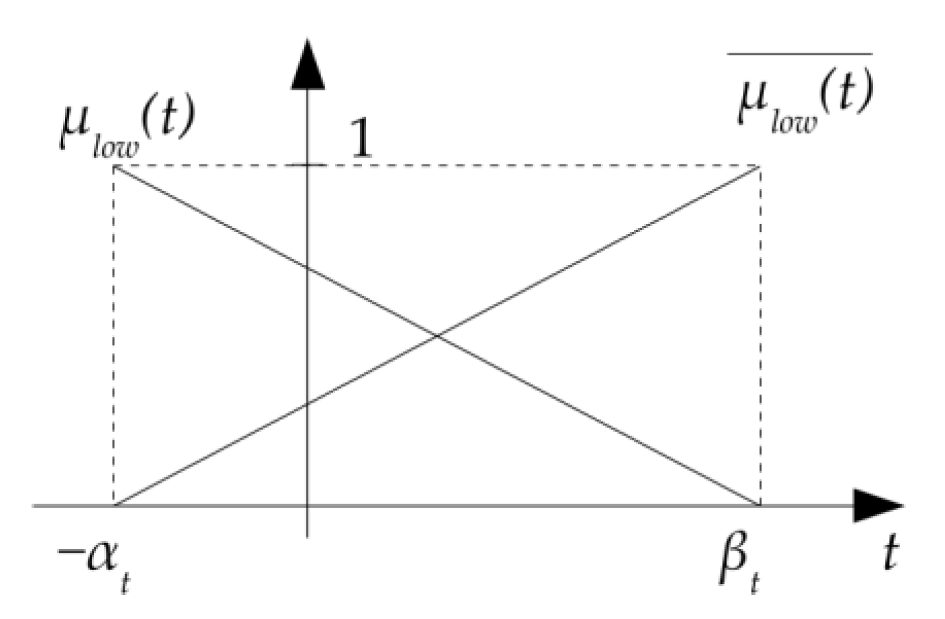
Equations (15)–(18) and the chart form the Figure 6 are citations from [20]. We place them here so that the reader can understand the method without the need for checking other publications. Similarly to Section 2.3, let us introduce the following linguistic variables: temperature t ∈ {low, }, insolationg ∈ {low, } and power P = {p1, p2, p3, p4}. Let us assume that the temperature and irradiation are bounded: t ∈ (−αt, βt), g ∈ (−αg, βg). For the given values of linguistic variables, let us define fuzzy sets shown below:

Figure 6.
The chart of the linear membership functions given by (12) and (13) [20].
Figure 6 shows the charts of the membership functions µlow(t) and . The values of the variable P will be real numbers. In [20], it is shown that with expressed conditions the zero-order Takagi-Sugeno system described by the following rules:
- IF t is low AND g is low THEN P = p1,
- IF t is AND g is low THEN P = p2,
- IF t is low AND g is THEN P = p3,
- IF t is AND g is THEN P = p4,
is equivalent to the following equation:
TS(t, g) = a·g·t + b·t + c·g + d.
Equations (3) and (19) define the same polynomial: they have a degree of 1 and both are functions of temperature and insolation. Therefore, the system can be modeled by (19) only when on the input there is given the temperature of the PV panel, not the air temperature.
2.5. Rule Based System—Nonlinear Membership Functions
As in Section 2.4, we cite Equation (20) and the chart from the Figure 7 from the work [20], where it was shown that using a certain class of nonlinear membership functions, it is possible to present a zero-order Takagi-Sugeno system as the scalar product of two matrices. Let us assume the following denotes:
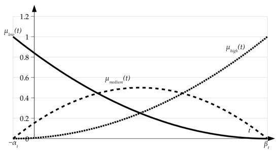
Figure 7.
The chart of nonlinear membership functions given by (20) for λ = 1 [20].
- Temperature, t ∈ {low, medium, high}
- Insolation, g ∈ {low, medium, high}
- Power, P ∈ {p1, p2, …, p9}
Suppose that temperature t ∈ (−αt, βt) and insolation g ∈ (−αg, βg), i.e., the values of temperature and solar radiation are limited to a certain range. For given values of linguistic variables, let us define fuzzy sets as follows:
where parameter λ satisfies the condition 0 < λ ≤ 1. In the further part of the discussion, we will assume that λ = 1. The chart of the membership functions µlow(t), µmedium(t) and µhigh(t) for the parameter λ = 1 is shown in Figure 7.
In [20], it was shown that with the given assumptions, the zero-order Takagi-Sugeno system described by the rules:
- IF t is low AND g is low THEN P = p1,
- IF t is medium AND g is low THEN P = p2,
- IF t is high AND g is low THEN P = p3,
- IF t is low AND g is medium THEN P = p4,
- IF t is medium AND g is medium THEN P = p5,
- …
- IF t is high AND g is high THEN P = p9,
is equivalent to the following equation:
where: n1, …, n9 are constant parameters. The Formula (21) is a generalization of polynomials (3), (7) and (8), so the system is able to model the daily production of energy with both air temperature and the panel temperature.
TS(t, g) = n1 · t2 · g2 + n2 · t2 · g + n3 · t2 + n4 · t · g2 + n5 · t · g + n6 ·t + n7 · g2 + n8 ·g + n9,
Using the test data file and the Matlab program similar to the one showed on the Algorithm 1, parameters of Equation (21) were computed. Table 4 contains obtained values.

Table 4.
Parameters of Equation (18) calculated from the training data set.
3. Results
This section presents the results of energy forecasting for developed models. The accuracy of the models was estimated on the bases of various forecast error measures.
3.1. Measures for Estimating Forecast Errors
In the literature on the problem of forecasting energy, the accuracy of prognostic models is determined by means of various measures. This often makes it difficult to compare the results of different authors and their prognostic methods. Therefore, it is advisable to present the obtained results in the form of standardized measures for calculating forecast errors. Thus, the accuracy of the models developed by us will be presented by using the error measures described below.
Mean error (ME):
Mean Absolute Error (MEA):
Mean Absolute Percentage Error (MAPE):
Root Mean Squared Error (RMSE):
Absolute Percentage Error (δP):
where is the measurement of energy in the solar installation on the i-th day, is the forecast of energy production on the i-th day, N is number of samples and ei = − Ei is the error of the forecast.
3.2. Forecast Errors Calculations
Table 5 presents the calculated errors of forecasts of particular models for the training data, where MP1 is the analytical model described by (7), MP2 is the analytical model described by (8), TSi is the ANFIS model described in Section 2.3, TS_nl is the Takagi-Sugeno fuzzy model with nonlinear membership functions given by (21). Table 6 presents forecast errors for the test data.

Table 5.
Forecasts errors for the training data.

Table 6.
Forecasts errors for the test data.
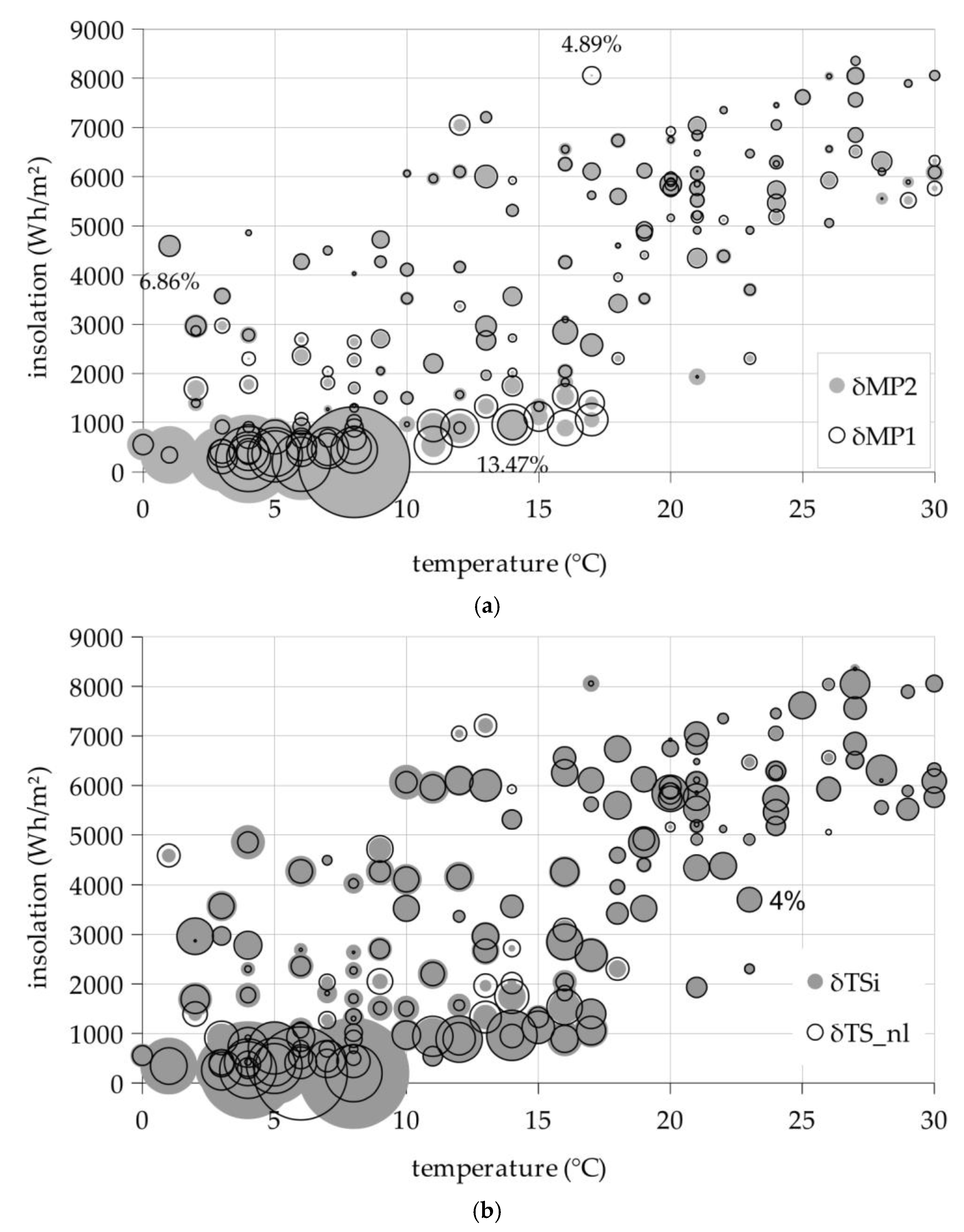
Figure 8a shows the distribution of the relative percentage errors (26) of energy forecasts for the MP1 and MP2 analytical models, marked as δMP1 and δMP2, in the test set. Figure 8b presents the distribution of the relative percentage errors of energy prediction for the TSi and TS_nl models, also in the test set. The areas of disks and areas enclosed by circles are proportional to values of errors. A gray disk included inside of the circle means that for the given pair (temperature, insolation), the model represented on the chart by the disk gives lower forecasting error comparing with the model represented by the circle. Figure 8 shows that every of investigated models has low forecasting quality for low temperatures and insolation values. Aggregated measures presented in Table 5 and Table 6 do not show these properties of models.
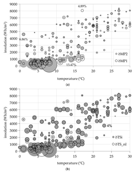
Figure 8.
Errors of approximation for the test data: (a) Equations (7) and (8) for MP1 and MP2 models; (b) TS system with triangular membership functions of the ANFIS model (δTSi) and the TS system with nonlinear membership functions given by Equation (21) (δTS_nl).
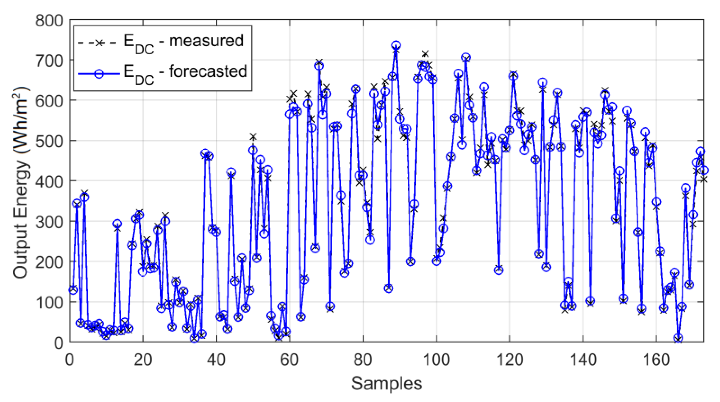
Figure 9 shows measured energy production and energy forecasts for the training data (174 days), and Figure 10 presents values energy measurements and forecasts for 173 days of the test data. Both charts allow to evaluate general quality of the model from Section 2.3 and show complexity of the PV panel energy production forecasting problem in the temperate climate area. Value of the forecasting energy for a succeeding day can be significantly different regardless of a season. The model correctly approximates training data (Figure 9) and keeps the quality for the test data (Figure 10).
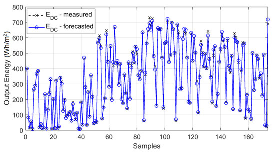
Figure 9.
The values of (EDC) energy measurements and (EDC) energy forecasts obtained from the ANFIS (TSi) model (the training data set, 174 days).
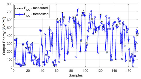
Figure 10.
The values of (EDC) energy measurements and (EDC) energy forecasts obtained from the ANFIS (TSi) model (the test data set, 173 days).
3.3. Conclusions and Discusion
After the comparison of the quality of measurement data interpolation of the acquired model with the analytical model from the references, one should draw the conclusion that such a system can be applied in forecasting (the TSi column in Table 5 and Table 6). Its performance is significantly better than that of analytical equations in all error measures. However, for one of the main error measures, namely, the MAPE error, the TS_nl rule system generates significantly smaller errors than the mathematical models and a little better than the ANFIS model.
On the basis of reference works in the area of applying analytical methods in fuzzy logic, it has been pointed out that the forecasting methods based on fuzzy logic are generalization of analytical equations, which depend on what membership function is applied to fuzzy sets. The best of the studied systems based on fuzzy logic, the analytical form of which is different than the discussed analytical equations, turn out to be better than the analytical equation (the TS_nl column in Table 5 and Table 6).
4. Software for Energy Production Forecast
Based of the above considerations, a prototype software for daily energy production forecast has been developed. The development platform is the CPDev engineering environment [31]. This platform allows to create control programs in languages of the IEC 61131-3 standard: structured chart (ST), instruction list (IL), ladder diagram (LD), functional block diagram (FBD) and sequential function chart (SFC). These programs can be deployed to different PLC devices and installed in solar panel sites. The forecasting software is currently at the Technology Readiness Level 3 (TRL) and consists of three main modules (see Figure 11a): the main program module, visualization panel management module and Human-Machine Interface (HMI) events processing module. Modules communicate by the use of global variables. The algorithm for the energy production forecast is as following (see Algorithm 2):
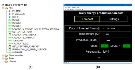
Figure 11.
(a) Structure of the program; (b) the Human-Machine Interface (HMI) in the CPVis the simulation environment.
- Get weather forecast (lines 9–11).
- Calculate the irradiation on the panel surface (lines 12–18).
- Calculate the energy production forecast (lines 19–23).
| Algorithm 2 The main function of the energy production forecast program. | |
| 1: | PROGRAM PR_MAIN |
| 2: | VAR_EXTERNAL (*$AUTO*) END_VAR |
| 3: | VAR |
| 4: | result: REAL; |
| 5: | weather_forecast_service: GET_WEATHER_FORECAST; |
| 6: | irradiation_service: IRRADIATION_IN_PANEL_SURFACE; |
| 7: | END_VAR |
| 8: | result := initialize(); |
| 9: | weather_forecast_service( |
| 10: | temperature => TEMPERATURE, |
| 11: | irradiationHorizontalSurface => IRRADIATION); |
| 12: | irradiation_service( |
| 13: | irradiation := IRRADIATION * 1e6, |
| 14: | latitudeOfTheSite := LATITUDE_OF_THE_SITE, |
| 15: | albedo := ALBEDO, |
| 16: | tiltAngle := TILT_ANGLE, |
| 17: | diffuseModel := DIFFUSE_MODEL, |
| 18: | irradiation_on_panel => IRRADIATION_ON_PANEL); |
| 19: | case FORECAST_MODEL_ID of |
| 20: | 0: result := MODEL1(MODEL_1_PARAMS,IRRADIATION_ON_PANEL,TEMPERATURE); |
| 21: | 1: result := MODEL2(MODEL_2_PARAMS,IRRADIATION_ON_PANEL,TEMPERATURE); |
| 22: | 2: result := MODEL3(MODEL_3_PARAMS,IRRADIATION_ON_PANEL,TEMPERATURE); |
| 23: | end_case |
| 24: | ENERGY_FORECAST := result; |
| 25: | END_PROGRAM |
The function of reading the weather forecast is currently being simulated but will be programmed as a custom function block, as described in the paper [32]. Two remaining functions are fully implemented. A calculation of the irradiation on the tilted PV panel surface is performed according to a previous paper [33]. Required parameters (albedo, diffusion model, solar panels total area, inverter efficiency, etc.) are entered in the settings panel (Figure 11b). Forecasting of the energy production is done by one of the three functions, MODEL1, MODEL2 and MODEL3, which implement Equations (7), (8) and (21), respectively. Coefficients of the mentioned equations are entered as constants in the settings panel.
5. Conclusions
The paper presents an overview of selected models of daily power production by photovoltaic panels. Parameters for individual models were computed and their quality assessed. The parameters of all model were determined in such a way as to ensure adjustment to the measurement data obtained from the photovoltaic system installation.
Studies have shown that the best model is a two-input Takagi-Sugeno system with nonlinear membership functions (TS_nl). Such a system is equivalent to a continuous linear function of two variables: insolation and temperature.
Noteworthy is the model described by Equations (7) and (8), because its quality is slightly lower than that of the TS_nl model, but its advantage is the low technical complexity and the existence of the analytical form of the model. The model can be used with both air and panel temperature. Since the latter quantity is not forecasted, it should be determined indirectly.
If you use the forecasts of insolation and temperature, the quality of forecasting power production depends on the quality of the weather forecast. Authors take the position that with a system model based on real measurements, one should strive to use high-quality forecasting data. With the development of weather forecasting methods, the quality of power output forecasts described in the paper will improve. High quality of the mentioned forecasts is related to the financing of green energy producers. A proper estimation of supply allows to gain a competitive advantage on the energy market.
Author Contributions
Conceptualization, D.M.; methodology, G.D. (Grzegorz Drałus) and G.D. (Grzegorz Dec); software, G.D. (Grzegorz Drałus) and G.D. (Grzegorz Dec); validation, B.K.; formal analysis, G.D. (Grzegorz Drałus) and G.D. (Grzegorz Dec); investigation, D.M., G.D. (Grzegorz Drałus) and B.K.; resources, D.M.; data curation, B.K.; writing—original draft preparation, D.M., B.K., G.D. (Grzegorz Drałus) and G.D. (Grzegorz Dec); writing—review and editing, D.M. and B.K.; visualization, B.K.; supervision, D.M.; project administration, D.M.; funding acquisition, D.M. All authors have read and agreed to the published version of the manuscript.
Funding
This project is financed by the statutory funds (UPB) of the Department of Electrical and Computer Engineering Fundamentals, Rzeszow University of Technology, and the Minister of Science and Higher Education of the Republic of Poland with in the “Regional Initiative of Excellence” program for years 2019–2022. Project number 027/RID/2018/19, total amount granted 11,999,900 PLN.
Data Availability Statement
Not applicable.
Conflicts of Interest
The authors declare no conflict of interest.
References
- Drałus, G.; Dec, G.; Mazur, D. One day ahead forecasting of energy generating in photovoltaic systems. In Proceedings of the Computing in Science and Technology (CST), ITM Web of Conferences, Rzeszów, Poland, 11–14 June 2018; Volume 21. [Google Scholar] [CrossRef]
- Piotrowski, P. Analysis of variable selection in the task of forecasting ultra-short-term production of electricity in solar systems. Electrotech. Rev. 2014, 90, 5–9. [Google Scholar]
- Mo, J.Y.; Jeon, W. How Does Energy Storage Increase the Efficiency of an Electricity Market with Integrated Wind and Solar Power Generation?—A Case Study of Korea. Sustain. J. Rec. 2017, 9, 1797. [Google Scholar] [CrossRef]
- Powell, K.M.; Hedengren, J.D.; Edgar, T.F. Dynamic optimization of a solar thermal energy storage system over a 24 hour period using weather forecasts. In Proceedings of the 2013 American Control Conference, Washington, DC, USA, 17–19 June 2013; pp. 2946–2951. [Google Scholar]
- Kudo, M.; Takeuchi, A.; Nozaki, Y.; Endo, H.; Sumita, J. Forecasting electric power generation in a photovoltaic power system for an energy network. Electr. Eng. Jpn. 2009, 167, 16–23. [Google Scholar] [CrossRef]
- Huang, Y.; Lu, J.; Liu, C.; Xu, X.; Wang, W.; Zhou, X. Comparative study of power forecasting methods for PV stations. In Proceedings of the 2010 International Conference on Power System Technology, Hangzhou, China, 24–28 October 2010; pp. 1–6. [Google Scholar]
- Nespoli, A.; Ogliari, E.; Leva, S.; Pavan, A.M.; Mellit, A.; Lughi, V.; Dolara, A. Day-Ahead Photovoltaic Forecasting: A Comparison of the Most Effective Techniques. Energies 2019, 12, 1621. [Google Scholar] [CrossRef]
- Yona, A.; Senjyu, T.; Saber, A.Y.; Funabashi, T.; Sekine, H.; Kim, C.-H. Application of neural network to 24-hour-ahead generating power forecasting for PV system. IEEE PES Gen. Meet. 2008, 1–6. [Google Scholar] [CrossRef]
- Dolara, A.; Grimaccia, F.; Leva, S.; Mussetta, M.; Ogliari, E. A Physical Hybrid Artificial Neural Network for Short Term Forecasting of PV Plant Power Output. Energies 2015, 8, 1138–1153. [Google Scholar] [CrossRef]
- Son, J.; Park, Y.; Lee, J.; Kim, H. Sensorless PV Power Forecasting in Grid-Connected Buildings through Deep Learning. Sensors 2018, 18, 2529. [Google Scholar] [CrossRef]
- Mei, F.; Pan, Y.; Zhu, K.; Zheng, J. A Hybrid Online Forecasting Model for Ultrashort-Term Photovoltaic Power Generation. Sustain. J. Rec. 2018, 10, 820. [Google Scholar] [CrossRef]
- Wang, F.; Zhen, Z.; Wang, B.; Mi, Z. Comparative Study on KNN and SVM Based Weather Classification Models for Day Ahead Short Term Solar PV Power Forecasting. Appl. Sci. 2017, 8, 28. [Google Scholar] [CrossRef]
- Ogliari, E.; Grimaccia, F.; Leva, S.; Mussetta, M. Hybrid Predictive Models for Accurate Forecasting in PV Systems. Energies 2013, 6, 1918–1929. [Google Scholar] [CrossRef]
- Kim, T.; Ko, W.; Kim, J.; Kim, T. Analysis and Impact Evaluation of Missing Data Imputation in Day-ahead PV Generation Forecasting. Appl. Sci. 2019, 9, 204. [Google Scholar] [CrossRef]
- Tephiruk, N.; Kanokbannakorn, W.; Kerdphol, T.; Mitani, Y.; Hongesombut, K. Fuzzy Logic Control of a Battery Energy Storage System for Stability Improvement in an Islanded Microgrid. Sustain. J. Rec. 2018, 10, 1645. [Google Scholar] [CrossRef]
- Kamel, A.A.; Rezk, H.; Shehata, N.; Thomas, J. Energy Management of a DC Microgrid Composed of Photovoltaic/Fuel Cell/Battery/Supercapacitor Systems. Batteries 2019, 5, 63. [Google Scholar] [CrossRef]
- Chang, E.-C. Study and Application of Intelligent Sliding Mode Control for Voltage Source Inverters. Energies 2018, 11, 2544. [Google Scholar] [CrossRef]
- Shadoul, M.; Yousef, H.; Abri, R.; Al-Hinai, A. Adaptive Fuzzy Approximation Control of PV Grid-Connected Inverters. Energies 2021, 14, 942. [Google Scholar] [CrossRef]
- Nguyen, A.-T.; Taniguchi, T.; Eciolaza, L.; Campos, V.; Palhares, R.; Sugeno, M. Fuzzy Control Systems: Past, Present and Future. IEEE Comput. Intell. Mag. 2019, 14, 56–68. [Google Scholar] [CrossRef]
- Kluska, J. Analytical Methods in Fuzzy Modeling and Control; Springer: Berlin/Heidelberg, Germany, 2009. [Google Scholar]
- Kim, S.-W.; Park, S.-Y.; Park, C. Spacecraft attitude control using neuro-fuzzy approximation of the optimal controllers. Adv. Space Res. 2016, 57, 137–152. [Google Scholar] [CrossRef]
- Smoczek, J. Experimental verification of a GPC-LPV method with RLS and P1-TS fuzzy-based estimation for limiting the transient and residual vibration of a crane system. Mech. Syst. Signal Process. 2015, 62–63, 324–340. [Google Scholar] [CrossRef]
- Kluska, J.; Hajduk, Z. Hardware Implementation of P1-TS Fuzzy Rule-Based Systems on FPGA. In Artificial Intelligence and Soft Computing; Rutkowski, L., Korytkowski, M., Scherer, R., Tadeusiewicz, R., Zadeh, L.A., Zurada, J.M., Eds.; ICAISC 2013. Lecture Notes in Computer Science; Springer: Berlin/Heidelberg, Germany, 2013; Volume 7894. [Google Scholar] [CrossRef]
- Sittón-Candanedo, I.; Alonso, R.S.; García, Ó.; Gil, A.B.; Rodríguez-González, S. A Review on Edge Computing in Smart Energy by means of a Systematic Mapping Study. Electronics 2019, 9, 48. [Google Scholar] [CrossRef]
- Gergaud, O.; Multon, B.; Ahmed, H.B. Analysis and Experimental Validation of Various Photovoltaic System Models. In Proceedings of the 7th International ELECTRIMACS Congress, Montréal, QC, Canada, 18–21 August 2002. hal-00674669. [Google Scholar]
- Durisch, W.; Bitnar, B.; Mayor, J.-C.; Kiess, H.; Lam, K.-H.; Close, J. Efficiency model for photovoltaic modules and demonstration of its application to energy yield estimation. Sol. Energy Mater. Sol. Cells 2007, 91, 79–84. [Google Scholar] [CrossRef]
- Ross, R.G. Interface design considerations for terrestrial solar cell modules. In Proceedings of the 12th Photovoltaic Specialists Conference, Conference Record (A78-10902 01-44), Baton Rouge, LA, USA, 15–18 November 1976; Institute of Electrical and Electronics Engineers, Inc.: New York, NY, USA, 1976; pp. 801–806. [Google Scholar]
- MATLAB Release 2012a (7.14.0.739); The MathWorks, Inc.: Natick, MA, USA, 2012.
- Bartman, J.; Kwiatkowski, B.; Mazur, D. The quality of data and the accuracy of energy generation forecast by artificial neural networks. Int. J. Electr. Comput. Eng. 2020, 10, 3957–3966. [Google Scholar]
- Jang, J.-S.R. ANFIS: Adaptive-network-based fuzzy inference system. IEEE Trans. Syst. Man Cybern. 1993, 23, 665–685. [Google Scholar] [CrossRef]
- Jamro, M.; Rzońca, D.; Sadolewski, J.; Stec, A.; Świder, Z.; Trybus, B.; Trybus, L. CPDev Engineering Environment for Modeling, Implementation, Testing, and Visualization of Control Software. In Advances in Intelligent Systems and Computing; Springer: Berlin/Heidelberg, Germany, 2014; Volume 267, pp. 81–90. [Google Scholar]
- Trybus, B. Development and Implementation of IEC 61131-3 Virtual Machine. Theor. Appl. Inform. 2011, 23, 21–35. [Google Scholar] [CrossRef][Green Version]
- Kamali, G.A.; Moradi, I.; Khalili, A. Estimating solar radiation on tilted surfaces with various orientations: A study case in Karaj (Iran). Theor. Appl. Clim. 2005, 84, 235–241. [Google Scholar] [CrossRef]
Publisher’s Note: MDPI stays neutral with regard to jurisdictional claims in published maps and institutional affiliations. |
© 2021 by the authors. Licensee MDPI, Basel, Switzerland. This article is an open access article distributed under the terms and conditions of the Creative Commons Attribution (CC BY) license (http://creativecommons.org/licenses/by/4.0/).

