Ocean Energy Systems Wave Energy Modeling Task 10.4: Numerical Modeling of a Fixed Oscillating Water Column

Abstract

This paper reports on an ongoing international effort to establish guidelines for numerical modeling of wave energy converters, initiated by the International Energy Agency Technology Collaboration Program for Ocean Energy Systems. Initial results for point absorbers were presented in previous work, and here we present results for a breakwater-mounted Oscillating Water Column (OWC) device. The experimental model is at scale 1:4 relative to a full-scale installation in a water depth of 12.8 m. The power-extracting air turbine is modeled by an orifice plate of 1–2% of the internal chamber surface area. Measurements of chamber surface elevation, air flow through the orifice, and pressure difference across the orifice are compared with numerical calculations using both weakly-nonlinear potential flow theory and computational fluid dynamics. Both compressible- and incompressible-flow models are considered, and the effects of air compressibility are found to have a significant influence on the motion of the internal chamber surface. Recommendations are made for reducing uncertainties in future experimental campaigns, which are critical to enable firm conclusions to be drawn about the relative accuracy of the numerical models. It is well-known that boundary element method solutions of the linear potential flow problem (e.g., WAMIT) are singular at infinite frequency when panels are placed directly on the free surface. This is problematic for time-domain solutions where the value of the added mass matrix at infinite frequency is critical, especially for OWC chambers, which are modeled by zero-mass elements on the free surface. A straightforward rational procedure is described to replace ad-hoc solutions to this problem that have been proposed in the literature.

1. Introduction

Wave energy converters (WECs) represent a small, but potentially significant, segment of the global renewable energy mix. In order to be competitive with offshore wind or solar power, however, the WEC sector will need to deploy reliable demonstration prototypes, paving the way to up-scaled commercialization and exploitation of economies of scale. This path requires accurate and reliable numerical modeling tools to allow for accurate evaluation of performance metrics during the initial design phases [1]. The International Energy Agency Technology Collaboration Program for Ocean Energy Systems (OES) was initiated in 2001 by Denmark, the United Kingdom, and Portugal, and now includes some 25 member countries. In 2016, the OES WEC modeling task was approved to assess the accuracy and reliability of numerical models for all aspects of WEC development. Initial results and conclusions from this work are reported in Reference [2], which focuses on two single degree-of-freedom point absorbers. The OES team agreed that the next step in this task would be to consider the modeling of Oscillating Water Column (OWC) devices, and this work is reported here. Of particular interest are OWC chambers designed to be integrated into a breakwater, as this is perhaps the most obvious and attractive first step for the large-scale commercialization of wave energy.

The OWC is the oldest, and arguably the most highly developed concept for exploiting ocean wave energy. OWCs have been used since the 1800s, first as whistling, and then electric, navigational buoys. Several shore-mounted installations have successfully contributed power to the electric grid for many years, and a number of floating prototypes have been launched and tested. Good reviews of the historical development of OWCs can be found in References [3,4]. More recently, a number of new designs have been developed for breakwater-mounted OWCs, many of which have been installed at various locations around the world. A good review of these developments is given in Reference [5]. For a good review of the general history of WEC development, we refer the reader to References [6,7].

The state of the art for the numerical modeling of WECs in general can be classified into three levels of refinement: linear and weakly-nonlinear potential flow theory (e.g., Reference [8]); fully-nonlinear potential flow theory (e.g., Reference [9]); and Computational Fluid Dynamics (CFD), solving the Navier–Stokes equations for either a single-phase or a two-phase fluid (see, e.g., Reference [10]). Predicting the response and energy absorption of an OWC-type device presents special challenges, both in terms of numerical modeling and model-scale experimental testing. The two main issues for scale-model testing are the effects of air compressibility, and the development of a good model for the behavior of the full-scale air turbine. A good discussion of these problems can be found in Reference [4]. The special challenges for numerical modeling are similarly mostly associated with correctly capturing the air-water interaction and possible air-compressibility effects. For weakly-nonlinear potential flow models, the interior chamber response is typically assumed to be a superposition of standing-wave modes. The hydrodynamic characteristics of these modes can be treated either through the introduction of so-called free-surface pressure (FSP) modes, as was done by Bingham et al. [11], or by treating the surface as a massless flexible plate and introducing generalized modes for the response of this plate [12]. Both methods require distributing panels directly on the free surface, which leads to singular matrices in the limit as the frequency $\omega \to \infty$. One of the contributions of this paper is to illustrate a simple method for accurately computing the added mass as $\omega \to \infty$, which is critical for time-domain modeling. This involves creating a new geometry for the device that is reflected about the $z=0$ plane and submerged to the original water depth, h, in a fluid of depth $2h$. In this way, we avoid any ad-hoc parameters associated with the finite-thickness plate methods that have been proposed in the past for solving this issue [13,14,15,16]. For CFD methods, the main issues are associated with properly resolving the two-phase fluid interaction between the water and air inside the chamber, in particular if the air phase is considered to be compressible.

The goal of this paper is to assess the accuracy of the current state of the art in numerical modeling of OWC-type WECs by comparison with a set of relatively large-scale experimental measurements for a breakwater-mounted OWC. These tests include only regular (monochromatic) incident waves that are of small amplitude with a maximum nonlinearity of about 15% of the maximum stable wave steepness. In reality, such a device would be exposed to irregular wave forcing, which complicates the analysis. In particular, for a weakly-nonlinear frequency-domain approach, a fixed wave-steepness value must be associated with each frequency component, which adds some uncertainty to the approach; whereas for CFD methods, properly resolving a large range of frequency components over a domain suited to the longer waves substantially increases the computational effort. This topic should be addressed in future work. Contributions to the study include several weakly-nonlinear potential flow solvers applying both incompressible- and compressible-flow models for the air phase, as well as several CFD solutions applying both compressible- and incompressible-flow assumptions. Unfortunately, we were not able to attract participants using fully-nonlinear potential flow. The calculations generally compare well with the experimental measurements for the amplitude of the primary-frequency, mean-chamber motion response and the pressure difference across the orifice plate, as well as the mean absorbed power. Air compressibility is found to be relatively unimportant for the flow through the orifice plate, but important for the interaction between the air volume in the chamber and the response of the internal chamber surface. This introduces a phase shift between the pressure and the elevation, which is captured by the weakly-nonlinear time-domain model; however, only the fully-nonlinear, compressible-flow CFD model is able to fully capture the detailed nonlinear chamber response. This highlights the need for a multi-level analysis strategy, where fast potential flow solutions are used to map out the response and target specific conditions for detailed analysis by much more expensive CFD calculations. Whether a fully-nonlinear potential flow model, with a compressible air-flow treatment, could also capture these details is an interesting question for future investigation.

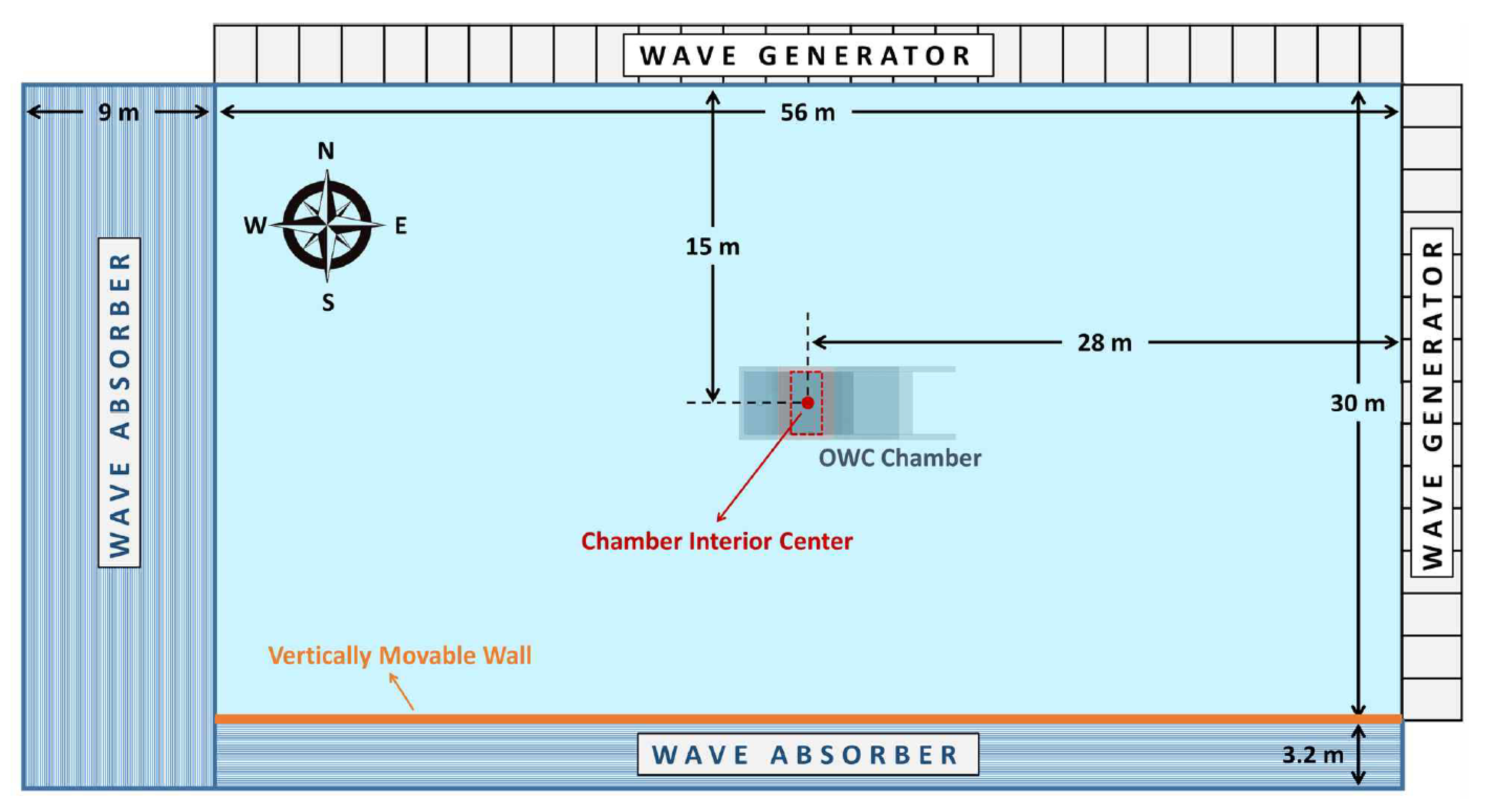
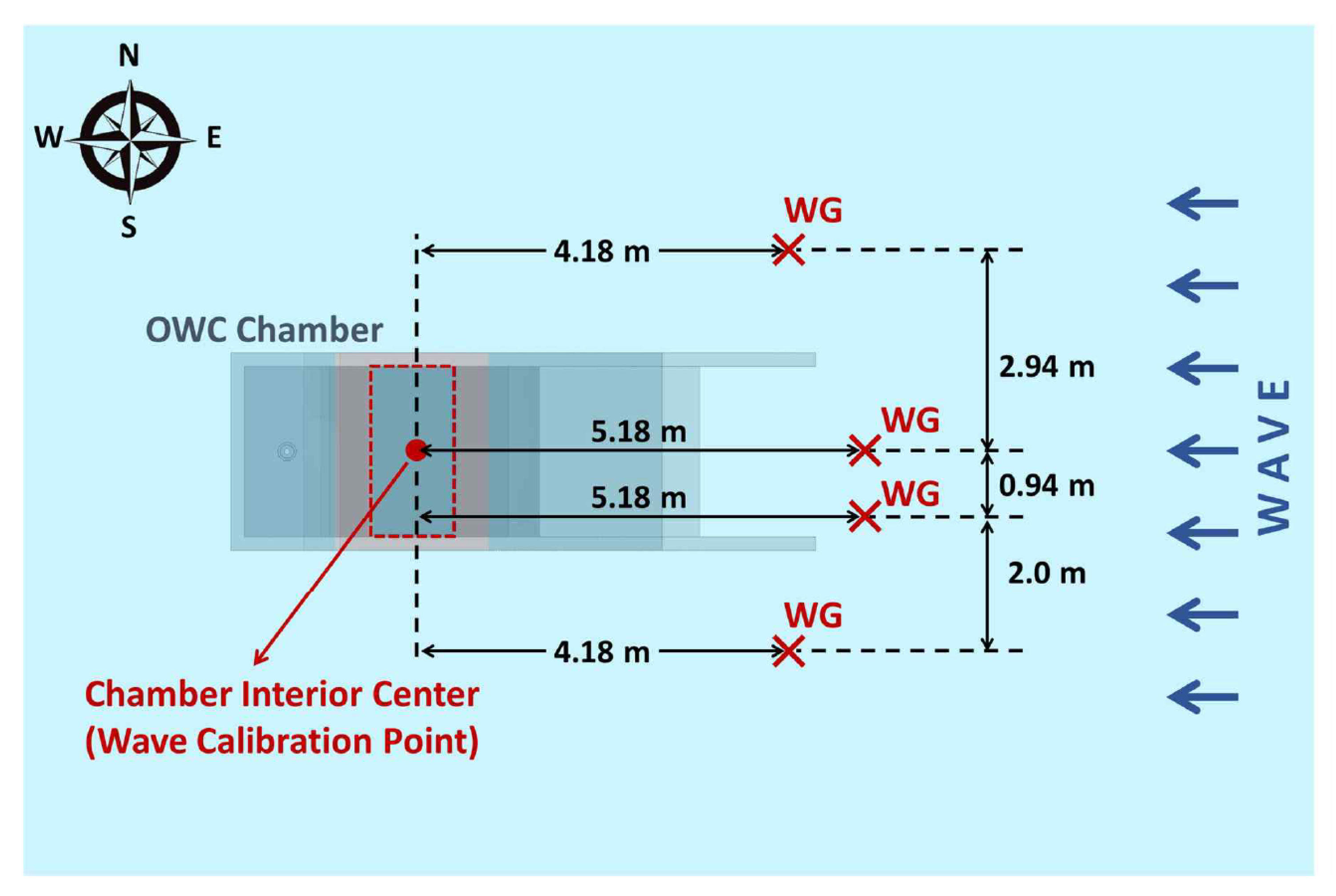
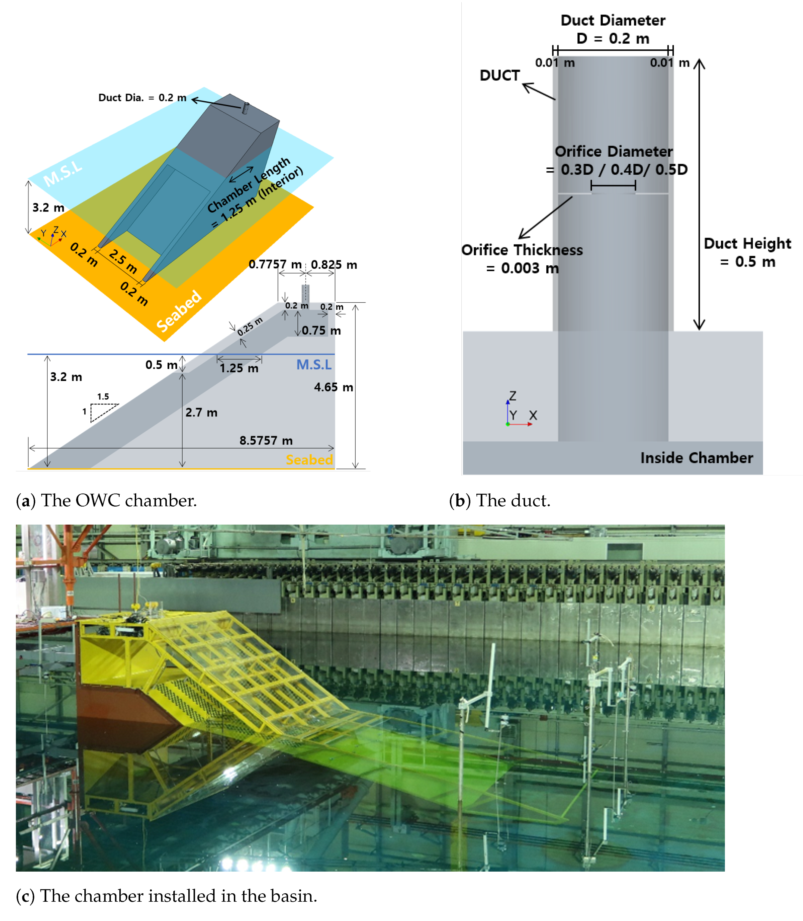
2. Experimental Measurements

The device was tested at a scale of 1:4 relative to a proposed full-scale deployment as part of a breakwater in a water depth of 12.8 m. The experimental measurements were carried out at the Korea Research Institute of Ships and Ocean Engineering (KRISO) ocean basin in 2019. Preliminary results along with a comparison to CFD calculations were presented in Reference [17]. The geometry and dimensions of the basin are shown in Figure 1, and the wave probe locations are indicated in Figure 2.

The wave conditions in terms of period T and height H are given in

Table 1. The experimental wave conditions.

WaveID	T [s]	H [m]	WaveID	T [s]	H [m]	WaveID	T [s]	H [m]
Low02	2.25	0.0450	Med02	2.25	0.0718	High02	2.25	0.1794
Low03	2.50	0.0467	Med03	2.50	0.0925	High03	2.50	0.2198
Low04	2.75	0.0459	Med04	2.75	0.0799	High04	2.75	0.1918
Low05	3.00	0.0464	Med05	3.00	0.0845	High05	3.00	0.1961
Low06	3.25	0.0454	Med06	3.25	0.0881	High06	3.25	0.1959
Low07	3.50	0.0440	Med07	3.50	0.0890	High07	3.50	0.2020
Low08	3.75	0.0480	Med08	3.75	0.0983	High08	3.75	0.2090

. As shown, three wave heights are used at each wave period, which are denoted by a WaveID of ‘Low’, ‘Med’ and ‘High’. The wave steepness values for each condition are shown in Figure 3 (left), which plots $H/\lambda$, with $\lambda$ the wavelength according to linear theory, along with the theoretical limiting value, $H_{max}$, given by the parameterized data of Reference [18]. Figure 3 (right) shows the steepness as a percentage of the maximum wave height, plotted against the relative water depth, $kh$, where $k=2\pi /\lambda$, showing that all of the wave conditions are nearly linear.

The geometry and dimensions of the chamber are shown in Figure 4. Also indicated in the figure are the dimensions of the air duct, which was fitted with orifice plates of three sizes to model the energy extraction from an air turbine. The chamber was fitted with nine wave gauges to measure the motion of the water column surface. Their locations are indicated in Figure 5, which also shows the locations of the six pressure sensors and the two hot wire anemometers that were installed in the duct. The wave gauges are capacitance-type gauges, manufactured in-house, with an accuracy of $\pm 1$ mm. The pressure gauges were connected to an Aplisens (Warsaw, Poland) model APR-2000ALW differential pressure transmitter that has a range of $\pm 2000$ Pa, with errors up to $\pm 0.075$% of the maximum differential pressure. The airflow speed through the duct was measured by two omnidirectional TSI (Shoreview, MN, USA) model number 8465 hot-wire anemometers. They have a range of 0 to 50 m/s with an uncertainty of up to $\pm 2.5$% of the maximum flow speed. All data were logged at 50 Hz.

Tests were performed with no orifice plate installed in the duct, and with three orifice plate sizes corresponding to $0.3D,0.4D$, and $0.5D,$ where $D=0.2$ m is the duct internal diameter.

Table 2. The experimental wave conditions. The cases marked by * indicate that the chamber elevations were too small to allow for synchronization of the signals.

TestID	Orifice	WaveID	TestID	Orifice	WaveID	TestID	Orifice	WaveID
402 *	$0.3D$	Med02	202 *	$0.5D$	Med02	302 *	$1.0D$	Med02
403	$0.3D$	Med03	203	$0.5D$	Med03	303	$1.0D$	Med03
404	$0.3D$	Med04	204	$0.5D$	Med04	304	$1.0D$	Med04
405	$0.3D$	Med05	205	$0.5D$	Med05	305	$1.0D$	Med05
406	$0.3D$	Med06	206	$0.5D$	Med06	306	$1.0D$	Med06
407	$0.3D$	Med07	207	$0.5D$	Med07	307	$1.0D$	Med07
408	$0.3D$	Med08	208	$0.5D$	Med08	308	$1.0D$	Med08
TestID	Orifice	WaveID	TestID	Orifice	WaveID	TestID	Orifice	WaveID
122 *	$0.4D$	Low02	102 *	$0.4D$	Med02	112	$0.4D$	High02
123	$0.4D$	Low03	103	$0.4D$	Med03	113	$0.4D$	High03
124	$0.4D$	Low04	104	$0.4D$	Med04	114	$0.4D$	High04
125	$0.4D$	Low05	105	$0.4D$	Med05	115	$0.4D$	High05
126	$0.4D$	Low06	106	$0.4D$	Med06	116	$0.4D$	High06
127	$0.4D$	Low07	107	$0.4D$	Med07	117	$0.4D$	High07
128	$0.4D$	Low08	108	$0.4D$	Med08	118	$0.4D$	High08

shows the conditions tested along with their TestID numbers. These conditions are meant to cover a wide range of possible operating conditions for the full-scale device.

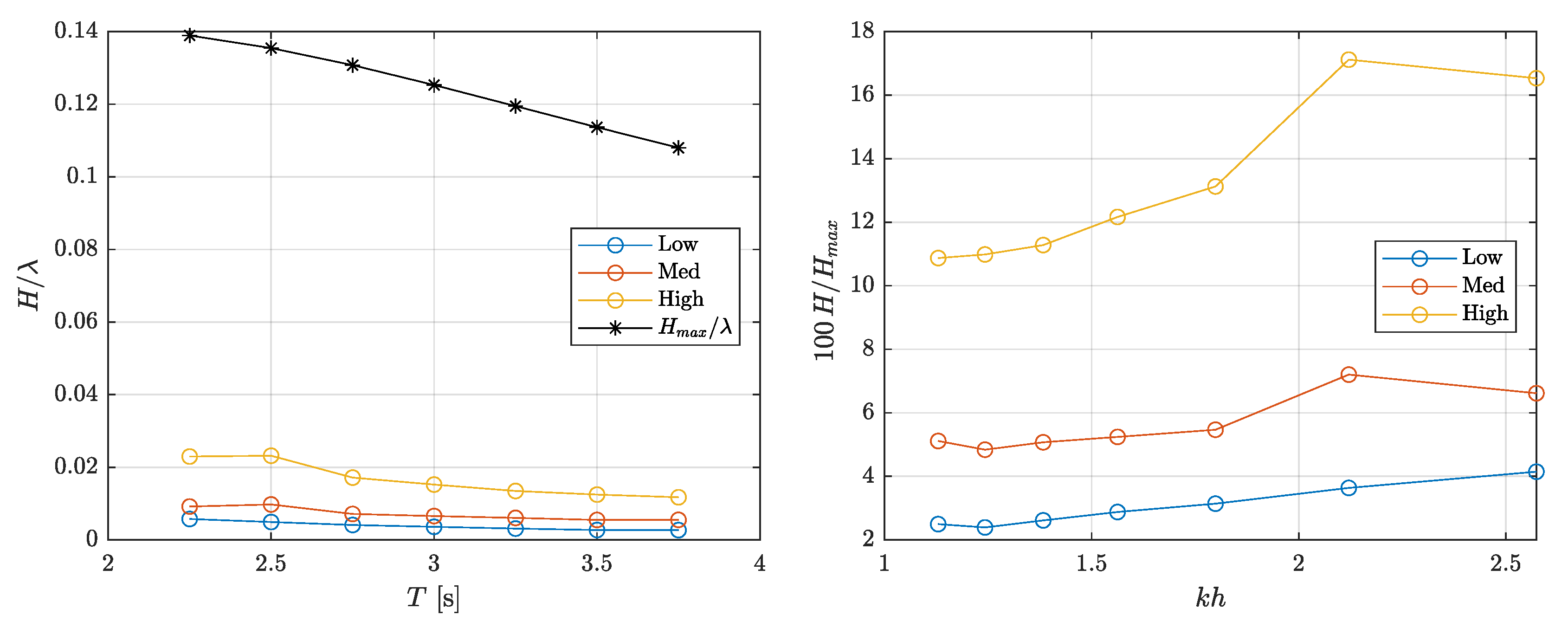
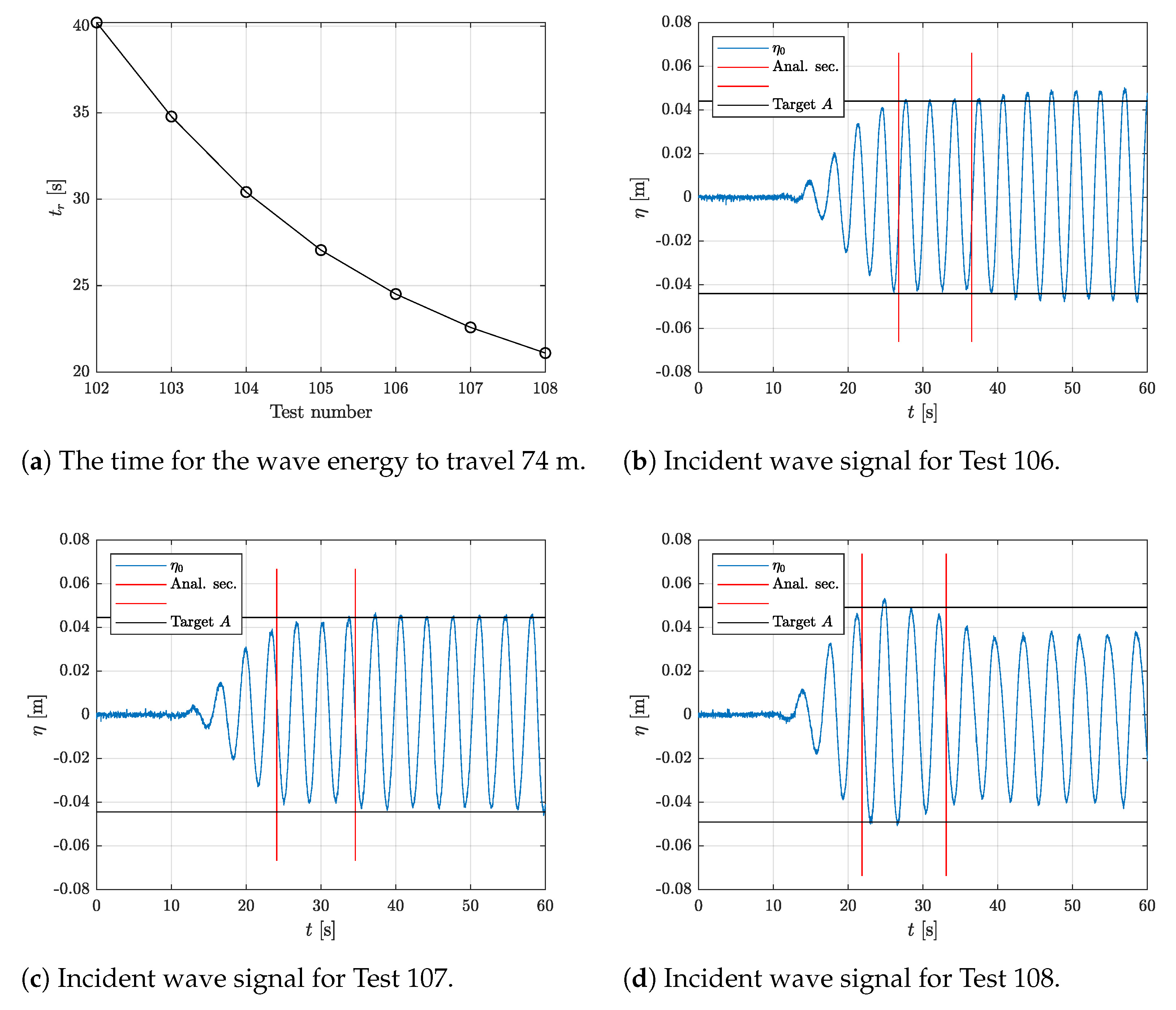
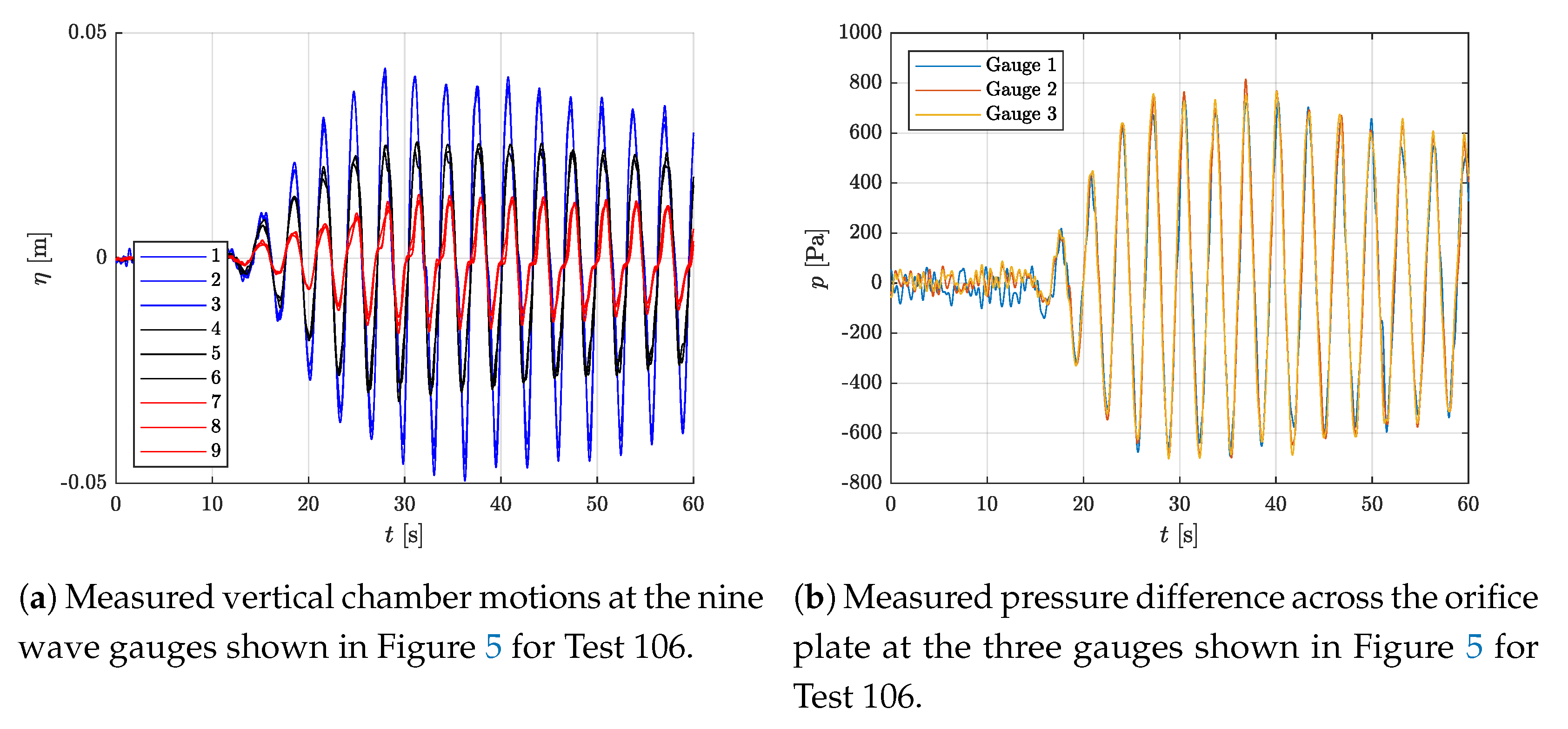
2.1. Analysis of the Experimental Data

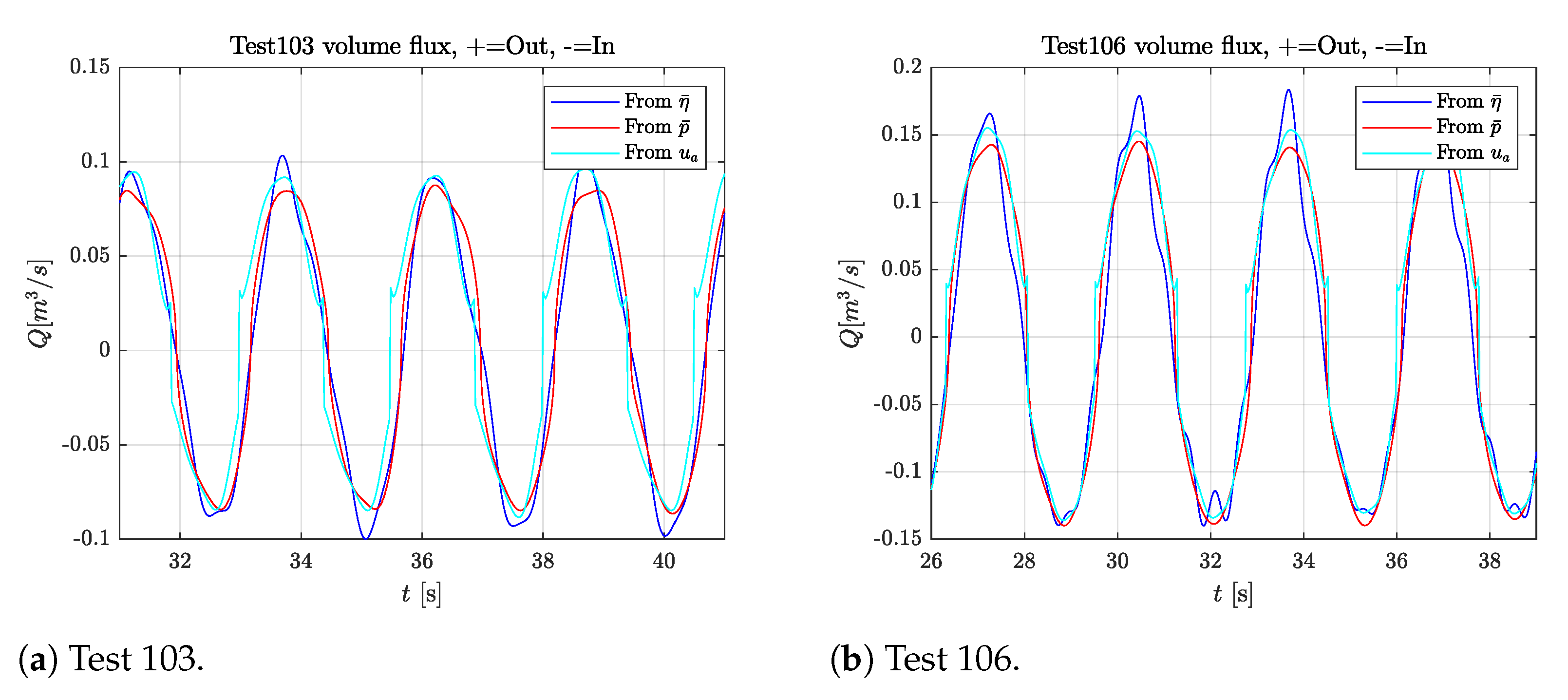
All of the tests shown in Table 2 were first performed without the chamber in place to establish the undisturbed incident wave conditions. For these tests, an additional probe was placed at the location of the center of the internal chamber, as indicated in Figure 5. Three examples of the measured incident wave signal in the open basin for Tests 106, 107, and 108 are shown in Figure 6, along with the chosen analysis section, and the target wave amplitude. The wavelengths here run from $\lambda =7.8$ m for WaveID 02 to $\lambda =17.8$ m for WaveID 08. Given that the length of the wave absorber is 9 m, we should expect wave reflections to become increasingly significant for the longer-wave cases. Also shown in this figure is an estimated time, $t_r$, for each wave to travel the 74 m from the chamber to the end of the beach and back again, based on the linear group velocity,

$$\begin{array}{ccc}\hfill c_g=\frac{c}{2}\left(1+\frac{2kh}{sinh2kh}\right),& {\displaystyle c=\frac{\omega }{k},}& {\omega }^2=gktanhkh,\hfill \end{array}$$

(1)

where c is the phase velocity, and $\omega =2\pi /T$ is the wave frequency. Considering the combination of $\lambda$ and $t_r$ for each case, WaveID 02 to 06 all provide a reliable, three to four wave period steady-state section for analysis without significant reflection effects. To extract the wave amplitude components, we make a linear least-squares fit of the signal over the analysis section to a sum of sinusoidal components at the primary wave frequency and the first four higher harmonics. In contrast to using a discrete Fourier transform, this technique is very robust and requires very few wave periods to accurately extract the harmonic components. This is verified by checking the residual of the fit and ensuring that it is at least several orders of magnitude smaller than the signal. For WaveID 07 and 08, reflections are clearly apparent during the chosen analysis section, but we have chosen to include them in the comparisons anyway, keeping in mind that they include additional uncertainty. This is justified by the observation that the departure from the target amplitude is relatively small during the analysis section, and that these cases are the most energetic of the series, thus being of interest in terms of air compressibility and nonlinear effects.

Figure 7 shows the internal-chamber, surface-elevation measurements and the measured pressure difference across the orifice plate for Test 106. Here, the chamber elevation, $\eta$, represents the vertical position of the water surface, i.e., the projection of the raw wave gauge distance to the vertical by multiplication with $sin\theta$, where $\theta =33.{69}^{\circ }$ is the chamber slope angle. In Figure 7a, we see that the three probe signals along each horizontal line are nearly identical, indicating that there is no significant transverse motion of the chamber water surface. On the other hand, we can identify a significant front-to-back standing wave oscillation from the relatively large differences in amplitude of the signals along each row of probes. In Figure 7b, we plot the pressure difference between each pair of pressure probes, so that Gauge 1 represents DP1–DP2, etc. A positive pressure difference, p, represents a greater pressure on the chamber side of the orifice plate than on the outside. Ideally, we would like to know the pressure difference between the chamber and the atmosphere, but the pressure differences between the chamber and the duct (and the duct and the atmosphere) are relatively small compared to the drop across the orifice plate. This conclusion is motivated by the following analysis.

First, we consider the effects of air compressibility. As long as the pressure differences are small compared to the atmospheric pressure, $p_a$, then a good approximation for the air density is given by

$$\rho ={\rho }_a\left(1+\frac{p}{\gamma p_a}\right),$$

(2)

where $\gamma =1.4$ is the heat capacity ratio, ${\rho }_a=1.225$ kg/m${}^3$, and $p_a=101,325$ Pa are the density and atmospheric pressure of air near sea level at 20 ${}^{°}$C. Figure 8 shows the variation in relative air density for Test 118, as estimated from Equation (2) and the measured pressure drop across the orifice plate. This case represents the largest measured pressure from the series and shows a maximum density variation of about 1.5%. From Figure 8, we might be tempted to conclude that compressibility effects should not be very significant for these experiments. However, as discussed further in Section 5.2, while air compressibility is not very important for the flow through the orifice, it leads to significant effects from the large-volume air chamber on the response of the chamber water surface.

As air flows from the chamber into the duct, it encounters a sudden pipe contraction, as discussed by Bullen et al. [19]. This is shown in Figure 9a, where $A_c$ is the area of the chamber water surface and $U_c$, $p_1$ are the mean air flow velocity and pressure in the chamber, whereas $A_d$ is the area of the duct, with $U_d$ and $p_2$ the corresponding mean velocity and pressure in the duct. Both of these control points are located away from any local disturbances caused by the contraction, so that the flows at these points are essentially homogeneous. Ignoring compressibility effects, and following Reference [19], we can write the Bernoulli equation for the pressure as

$$p_1+\frac{1}{2}\rho U_c^2=p_2+\frac{1}{2}\rho U_d^2+K_c\frac{1}{2}\rho U_d^2,$$

(3)

where $K_c$ is a pressure loss coefficient representing the head loss through the contraction. Figure 2 from Reference [19] sketches the situation showing how, in a real flow (i.e., Reynolds number less than infinity), $K_c$ consists of several contributions from the contraction phase as the flow enters the duct and from the expansion phase as the flow recovers again downstream of the transition. From mass conservation, the volume flux is $Q=U_c{A}_c=U_d{A}_d$. Using this in Equation (3), we can express the pressure drop across the contraction as

$$\begin{array}{ccc}\hfill p=p_1-p_2& {\displaystyle =\frac{1}{2}\rho \left(\frac{K_c+1}{{\sigma }^2}-1\right)U_c^2=}& \frac{1}{2}\rho \frac{1}{{\left(C_d\sigma \right)}^2}{U}_c^2,\hfill \end{array}$$

(4)

where $\sigma =A_d/A_c$ is the area ratio, and we have introduced the coefficient

$$C_d=\sqrt{\frac{1}{K_c+1-{\sigma }^2}}.$$

(5)

Considering a typical case from these experiments, the peak chamber velocity is $U_c=0.05$ m/s, which gives a chamber Reynolds number of $R=U_c{L}_1/\nu \approx 8500$. Using the model derived in Reference [19] gives $C_d=0.8356$ for this case. This gives a maximum pressure drop of about 20 Pa for the most energetic tests, which is less than 1% of the maximum pressure drop across the orifice plate with a diameter of $0.4D$. We can expect a similar effect as the flow passes from the duct to the atmosphere. Thus, for the cases that we focus on here, we can conclude that the measured pressure drop is very close to the pressure drop between the chamber and the atmosphere.

For the flow across the orifice plate, the situation is sketched in Figure 9b. Again, considering two control points located away from local disturbances due to the orifice plate, we can write the Bernoulli equation as

$$\begin{array}{ccc}\hfill p_2+\frac{1}{2}\rho U_d^2=& {\displaystyle p_3+\frac{1}{2}\rho U_d^2+K_c\frac{1}{2}\rho U_d^2}& \hfill \\ \hfill \to p=p_2-p_3=& {\displaystyle \frac{1}{2}\rho K_c{U}_d^2}& =\frac{1}{2}\rho \frac{1}{{\left(C_d\sigma \right)}^2}{U}_d^2,\hfill \end{array}$$

(6)

where, in this case, $\sigma =A_o/A_d$ is the ratio of the orifice area to the duct area and the total pressure loss across the orifice is expressed by the pressure loss coefficient, $K_c$. From the experimental measurements, the estimated value corresponds to $C_d=0.82$. Using this value, and mass conservation, we can compare estimates of the volume flux in the chamber from each of the three measurements:

• $Q=A_c\overline{u}$, where $\overline{u}={\partial }_t\overline{\eta }$, with $\overline{\eta }$ the mean of the nine internal wave gauge measurements and ${\partial }_t$ the time derivative (here taken by a fourth-order finite-difference scheme).
• $Q=A_o{u}_a$, where $u_a$ is the measured air flow velocity through the orifice. Here, it was determined that the most accurate result was found by taking the value from the upper gauge for the outflow and from the lower gauge for the inflow.
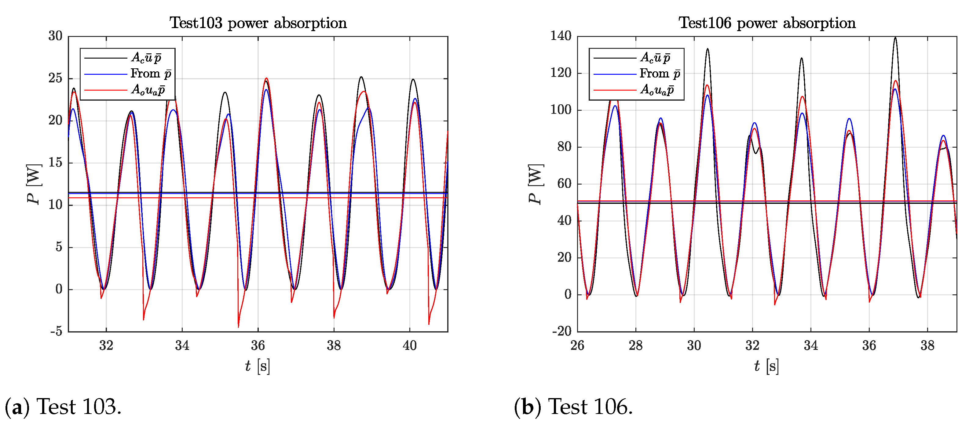
• From Equation (6), we can write $Q=\sqrt{2{\left(C_d{A}_o\right)}^2/\rho \left|\overline{p}\right|}\mathrm{sign}\left(\overline{p}\right)$, where $\overline{p}$ is the mean of the three pressure difference measurements.

Two examples are shown in Figure 10, where we can see reasonably good agreement between the predictions from the three measurements.

The absorbed power is given by $P=Qp$, so there are nine possible ways to estimate absorbed power from the three experimental measurement quantities. In order to minimize the use of the empirical pressure-flux relation, Equation (6), we chose to focus on the three of these given by the previously described estimates of Q and the average of the measured pressures, $\overline{p}$. Figure 11 shows two examples for Tests 103 and 106. The mean absorbed power, per wave cycle, is indicated by the horizontal lines.

3. Numerical Modeling of OWC Chambers

This section describes the numerical models that have been applied in this study to predict the KRISO OWC chamber response and power absorption. Three levels of modeling have been applied, corresponding to: weakly-nonlinear potential flow theory in the frequency domain, weakly-nonlinear potential flow theory in the time domain, and CFD. Both compressible- and incompressible-flow models are applied to the air phase. These models are outlined in the following subsections.

3.1. Weakly-Nonlinear Potential Flow Theory in the Frequency Domain

Detailed presentations of linearized, potential flow theory for the analysis of wave-structure interaction can be found in the classic textbooks by Newman, Falnes, or Faltinsen [20,21,22]. Here, we will summarize the theory and define the notation used. In order to apply radiation/diffraction theory to OWC chambers, there are two standard approaches. The first approach follows that outlined in References [21,23,24,25], in which new degrees of freedom are introduced to represent the pressure distribution applied to the interior free surface of each chamber by the air turbine. This approach is implemented in the software WAMIT [26], under the label Free-Surface Pressure (FSP) modes, and it was applied to the analysis of a fixed OWC chamber by Reference [11]. A second approach, which is more straightforward to apply in the time domain, is to treat the interior free surface of the chamber as a massless element of the structural boundary, which is free to move in a set of predefined generalized modes. This approach is described in Reference [27] and is also implemented in WAMIT. When generalized modes are included, the equations of motion for a floating structure can be written as

$$\begin{array}{ccc}\hfill \sum _{k=1}^{6+M_g}\left[-{\omega }^2\left(M_{jk}+A_{jk}\right)+\mathrm{i}\omega \left(B_{jk}+B_{jk}^0\right)+c_{jk}\right]{\xi }_k=& X_j,& j=1,2,\dots ,6+M_g.\hfill \end{array}$$

(7)

Here, ${\xi }_j\left(\omega \right)$ is the generalized body-response phasor in $6+M_g$ degrees of freedom, where $j=1,2,3$ correspond to translational motions in surge, sway, and heave, $j=4,5,6$ represent rotational motions in roll, pitch, and yaw, and $j=7,8,\dots ,6+M_g$ describe the motions of the interior chamber surface. Each generalized mode is defined by the boundary conditions

$$\begin{array}{ccc}\hfill \left.\begin{array}{ccc}\frac{\partial {\varphi }_j}{\partial z}=& w_j\left(\mathbf{x}\right),& \mathrm{on}{S}_i\\ \frac{\partial {\varphi }_j}{\partial n}=& 0,& \mathrm{on}{S}_b\end{array}\right\}& & j=7,8,\dots ,6+M_g,\hfill \end{array}$$

(8)

where ${\varphi }_j$ is the radiation potential in mode j, $w_j\left(\mathbf{x}\right)$ defines the vertical displacement of the interior free surface due to unit amplitude motion in mode j, $S_i$ is the internal free surface, $S_b$ is the submerged body surface, and $\partial /\partial n$ represents the derivative in the direction normal to $S_b$. $M_{jk}$ is the linearized body inertia matrix, $A_{jk}\left(\omega \right)$ and $B_{jk}\left(\omega \right)$ are the radiation added mass and damping coefficient matrices, $c_{jk}$ is the hydrostatic restoring coefficient matrix, and $X_j\left(\omega \right)$ is the diffraction exciting force coefficient vector. The assumption here is that the incident wave can be described by a superposition of linear Stokes waves at frequency $\omega$ of the form

$$\begin{array}{ccc}\hfill {\eta }_0(\mathbf{x},t)& =& \Re \left\{A{\mathrm{e}}^{\mathrm{i}[\omega t-k(xcos\beta +ysin\beta \left)\right]}\right\}\hfill \end{array}$$

(9)

$$\begin{array}{ccc}\hfill {\varphi }_0(\mathbf{x},z,t)& =& -\Re \left\{\mathrm{i}\frac{gA}{\omega }\frac{coshk(z+h)}{coshkh}{\mathrm{e}}^{\mathrm{i}[\omega t-k(xcos\beta +ysin\beta \left)\right]}\right\}.\hfill \end{array}$$

(10)

Here, $\Re \left\{\right\}$ indicates the real part of a complex quantity, $\mathbf{x}=[x,y]$ is a horizontal position vector, and the z-axis is oriented vertically upward, with $z=0$ at the still-water level and $z=-h$ at the fluid bottom. The free-surface elevation is ${\eta }_0$ and ${\varphi }_0$ is the velocity potential, with g the gravitational acceleration. The incident wave has a period $T=2\pi /\omega$, a length $\lambda =2\pi /k$, an amplitude $A=H/2$, and it propagates in the direction defined by the angle $\beta$, measured from the positive x-axis. The dispersion relation, Equation (1), relates the wave period and length, and defines the wave phase and group velocities c and $c_g$. All the coefficients appearing in Equation (7) can be computed for any desired floating structure using, for example, the frequency-domain radiation/diffraction code WAMIT [26], except for the matrix $B_{jk}^0$, which represents the damping applied to the chamber motion by the power-extracting air turbine, or in this case the orifice plate. The evaluation of $B_{jk}^0$ is discussed in Section 3.3, and, because the applied damping is a nonlinear function of the chamber flux, its inclusion in the otherwise linear equations makes them weakly-nonlinear.

3.2. Weakly-Nonlinear Potential Flow Theory in the Time Domain

As originally noted by Cummins [28], the frequency-domain formulation described earlier has an equivalent statement in the time domain. A weakly-nonlinear version of this formulation can be written as

$$\begin{array}{cc}\hfill \sum _{k=1}^{6+M_g}\left[(M_{jk}+A_{jk}^{\infty }){\ddot{x}}_k\left(t\right)+{\int }_{-\infty }^t{K}_{jk}(t-\tau ){\dot{x}}_k\left(\tau \right)d\tau +c_{jk}{x}_k\left(t\right)\right]=F_{jD}+F_{j0},& \\ \hfill j=1,2,\dots ,6+M_g,\end{array}$$

(11)

where $x_j\left(t\right)$ is the time history of the motion response in mode j, $A_{jk}^{\infty }=A_{jk}(\infty )$ is the infinite frequency limit of the added mass, and the over-dots represent time differentiation. The radiation impulse response functions, $K_{jk}$, and the diffraction exciting forces, $F_{jD}$, are related to the frequency-response functions by the Fourier transforms

$$\begin{array}{ccc}\hfill K_{jk}\left(t\right)=& {\displaystyle \frac{2}{\pi }{\int }_0^{\infty }{B}_{jk}cos\omega td\omega ,}& K_{jD}\left(t\right)=\frac{1}{2\pi }{\int }_{-\infty }^{\infty }{X}_j{\mathrm{e}}^{\mathrm{i}\omega t}d\omega ,\hfill \end{array}$$

(12a)

$$\begin{array}{ccc}\hfill F_{jD}\left(t\right)=& {\displaystyle {\int }_{-\infty }^{\infty }{K}_{jD}(t-\tau )\eta \left(\tau \right)d\tau }& ={\int }_{-\infty }^{\infty }\frac{X_{jD}}{A}\widehat{\eta }{\mathrm{e}}^{-\mathrm{i}\omega t}d\omega ,\hfill \end{array}$$

(12b)

$$\begin{array}{cc}\hfill \widehat{\eta }\left(\omega \right)=& {\displaystyle {\int }_{-\infty }^{\infty }\eta \left(t\right){\mathrm{e}}^{\mathrm{i}\omega t}dt,}\end{array}$$

(12c)

where $\eta$ is a particular incident wave elevation measured at the origin of the coordinate system. Here, $K_{jD}$ is the diffraction impulse response function, and the two equivalent forms of $F_{jD}$ indicate how the wave excitation force can be computed in either the time or the frequency domains, when the incident wave elevation signal is known for all time. Other external forces applied to the body, for example by the air turbine or a mooring system, are represented by $F_{j0}\left(t\right)$ and can be nonlinear.

3.3. Potential Flow Modeling of the Orifice Plate Damping—Incompressible Flow

Under the assumption that air compressibility effects are negligible, Equation (6) defines the relation between the flux in the chamber, Q, and the pressure difference across the orifice plate, p,

$$p\left(t\right)=\frac{1}{2}{\rho }_a{\left(\frac{1}{C_d{A}_o}\right)}^{2}Q{\left(t\right)}^2\mathrm{sign}\left(Q\right).$$

(13)

Defining generalized mode $j=7$ to be the piston mode (uniform vertical motion of the chamber surface), the flux is $Q=A_c{\dot{x}}_7$, with $A_c$ the chamber free-surface area. The force applied by the orifice plate is then

$$\begin{array}{ccc}\hfill F_{70}=-A_c{R}_0{\dot{x}}_7^2\mathrm{sign}\left({\dot{x}}_7\right),& & R_0=\frac{1}{2}{\rho }_a{\left(\frac{A_c}{C_d{A}_o}\right)}^2.\hfill \end{array}$$

(14)

As long as all other mode shapes are defined to have zero mean value, they will not contribute to the flux, and thus not directly experience any forcing from the orifice plate.

Equation (14) can be applied directly in the time-domain model, but in the frequency domain an equivalent linearized damping coefficient must be developed. For example, as shown in Reference [11], assuming a sinusoidal flux at frequency $\omega$, and a linear relationship between the pressure and the flux gives

$$B_{77}^0=\frac{8}{3\pi }\omega A_c{R}_0\left|{\xi }_7\right|,$$

(15)

as the equivalent linear damping coefficient that ensures the same power extraction per cycle as that defined by Equation (14). Because this damping coefficient depends on the chamber motion response, ${\xi }_7$, the solution to Equation (7) is also weakly nonlinear and must be found iteratively for each combination of frequency and incident wave steepness, $ϵ=2A/\lambda$.

3.4. Potential Flow Modeling of the Orifice Plate Damping—Compressible Air Volume with Incompressible Orifice Flow

As discussed in Section 2.1, the effects of air compressibility in these experiments are small but significant, suggesting that, at full scale, such compressive effects cannot be neglected. This is also discussed, for example, by Kelly et al. [29] and Sheng et al. [30]. In the current work, the influence of the air compressibility on the potential flow models of an OWC is considered from the perspective of the volume of air contained within the OWC above the water column and separately from the perspective of the air flow between the air volume and atmosphere through the orifice. A relationship between the pressure in the air chamber with respect to both the mass flow of air into or out of the chamber and the variation in the water column displacement, and in which the compressibilty of air within the chamber is considered, may be obtained from the First Law of Thermodynamics, and is given [31] by

$$\dot{p}=\frac{c_s^2}{V}\dot{m}-\frac{\gamma p}{V}\dot{V},$$

(16)

where V is the volume of air in the chamber above the water column, and $c_s$ is the speed of sound in air. Assuming air is an ideal gas, $c_s^2=\gamma p/\rho$, and the change in air density due to the compression of air may be obtained from Equation (2). The air flow direction, either into or out of the chamber, is dependent on the value of p. If the flow through the orifice is considered incompressible, then orifice theory may be used to model the mass flow of air into or out of the OWC chamber, as given in Equation (17)

$$\dot{m}=-C_d{A}_o\sqrt{2{\rho }_a\left|p\right|}\mathrm{sign}\left(p\right).$$

(17)

The force acting on the water column due to the pressure differential between the air trapped in the OWC chamber above the water column, and atmospheric pressure is $F_{70}=p{A}_c$. The pressure differential p is assumed to act uniformly over the surface of the water column and is treated as a state variable in the time-domain state-space model discussed in Section 4.3.

3.5. Potential Flow Modeling of the Orifice Plate Damping—Compressible Air Volume with Compressible Orifice Flow

If the flow of air through the orifice is also considered compressible, Equation (16) may still be used to model the pressure variation within the OWC chamber, while Equation (17) may be modified to allow for the expansion of gases flowing from a region of higher pressure to a region of lower pressure. Under unchoked conditions, the mass flow rate through an orifice may be given [32] by

$$\dot{m}=\frac{C_d}{\sqrt{(1-{\sigma }^4)}}{A}_o\sqrt{2{\rho }_1{p}_1\left(\frac{\gamma }{\gamma -1}\right)\left[{\left(\raisebox{1ex}{$p_2$}\!\left/ \!\raisebox{-1ex}{$P_1$}\right.\right)}^{\left(\raisebox{1ex}{$2$}\!\left/ \!\raisebox{-1ex}{$\gamma $}\right.\right)}-{\left(\raisebox{1ex}{$p_2$}\!\left/ \!\raisebox{-1ex}{$P_1$}\right.\right)}^{\left(\raisebox{1ex}{$\gamma +1$}\!\left/ \!\raisebox{-1ex}{$\gamma $}\right.\right)}\right]},$$

(18)

where $\sigma =A_o/A_d$, $p_1$, and ${\rho }_1$ are the pressure and density of the fluid in the region of higher air pressure, and $p_2$ is the fluid pressure in the region of lower air pressure.

3.6. Numerical Potential Flow Solutions

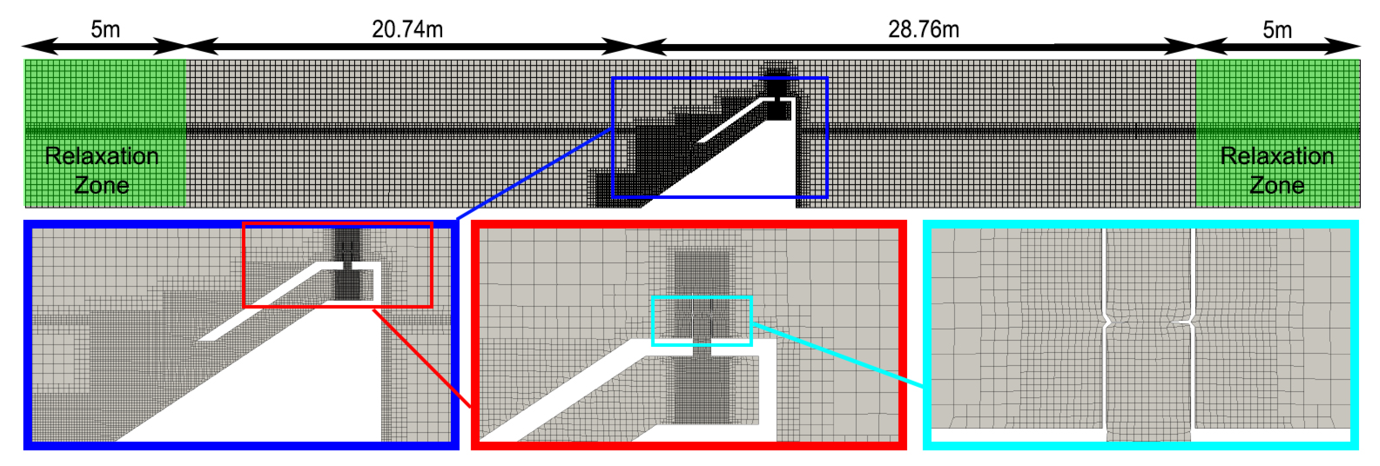
All of the participants in this study who used a potential flow assumption started by computing the coefficients appearing in Equation (7) using the high-order Boundary Element Method (BEM) solver, WAMIT [26]. Complete details on this software can be found in the WAMIT user manual and associated references on the web page. Analyzing OWC chambers with this technique presents some special challenges, which are discussed in the following subsections.

For the generalized modes representing the motion of the internal chamber surface ($j>6$), the inertia terms, $M_{jk}$, are all zero; therefore, it is of critical importance to have an accurate estimate of $A_{jk}^{\infty }$ in order to solve the problem in the time domain. Unfortunately, when the body has panels lying directly on the free surface, the integral equation is, in fact, singular [33]. Thus, the infinite-frequency problem for OWC-type modes cannot be solved in the usual way using a standard radiation/diffraction BEM, such as WAMIT. This failure has been noted by several authors and was studied in some detail by Sheng et al. [13], who suggested replacing the zero-mass (zero-thickness) internal free surface with a light piston of small finite displacement, which makes the calculation of $A_{jk}^{\infty }$ non-singular. A number of other authors have also used this approach; recent examples include References [14,15,16]. However, there are two problems with this approach. First, it is not obvious that the finite-mass floating piston is a good representation of the true free surface, nor how heavy the piston should be made to find a good balance between modeling the chamber motion and computing $A_{jk}^{\infty }$ accurately. Second, even if this gives a good representation of the piston mode, what about the other possible modes of motion for the internal free surface? In other words, it is surely possible, with some effort, to tune this approach to a particular chamber and get reliable results, but it is an ad-hoc and theoretically questionable method.

Instead of this ad-hoc approach, we suggest a more reliable and straightforward method. For a given OWC geometry, the finite-frequency values of the added mass and damping coefficients are computed as usual. Then, a new geometry is constructed by reflecting the original submerged geometry about the $z=0$ plane. The patches/panels that describe the interior free surface are then redefined as dipole patches [26], and the body is submerged to the original water depth, h, while the depth is redefined to be $2h$. Now the infinite (and zero) frequency problems can be solved accurately and reliably, and the results (divided by two) combined with the originally computed finite-frequency values. This strategy also ensures that $A_{jk}^{\infty }$ is correctly computed for all generalized modes defined on the chamber free surface, as well as the coupling between all rigid-body and generalized modes.

Figure 12 shows the two KRISO chamber geometries used here. These geometries have been created using the analytic geometry feature of WAMIT by including a dedicated subroutine that is linked to the WAMIT executable at run-time. The body-coordinate system has its origin at the center of the interior chamber surface, with the x-axis pointing toward the incoming waves. The first patch of the geometry (shown in green in Figure 12) represents the internal chamber free surface. To model the motions of the chamber water column, a corresponding set of generalized modes has been added to the newmodes.f file to describe the vertical motions of the chamber surface. These modes are of the form

$$\begin{array}{ccc}\hfill w_m\left(x\right)=cos\left[m{k}_l(x-x_0)\right],& m=0,1,\dots ;& k_l=\frac{\pi }{L_c},\hfill \end{array}$$

(19)

where $L_c=1.25$ m is the x-length of the interior free surface, and $x_0$ is the position of the front wall of the chamber in the body-coordinate system. After comparing solutions using four modes and then two modes, it was determined that, over the range of wave frequencies of interest here, the higher-mode responses are very small and do not influence the first two modes of motion. Thus, we include only $m=0$ (the piston mode) and $m=1$, the first sloshing mode. These modes correspond to $j=7,8$, respectively. Figure 13 illustrates how the two-mode approximation of the internal surface motion relates to the geometry of the chamber. The solid black lines indicate the internal walls of the chamber, and the dashed red line shows the still water surface. Although, in reality, the water surface will follow the sloped chamber walls, linear theory assumes that the motion is vertical, following the dashed black lines. The dashed green lines indicate the front and back set of wave probes, which are offset by a distance of $s_l=0.46875$ m from the chamber centerline. The dotted blue line indicates the piston mode, and the solid blue line the sum of the piston and the first sloshing-wave modes.

Three grids have been run to ensure converged results. These are labeled Grids 1–3 and correspond to setting PANEL_SIZE = [1, 0.5, 0.25] m. The resulting added mass and damping coefficients are shown in Figure 14, where we note that the $\omega =\infty$ limit is plotted at $\omega \sqrt{L/g}=4$, with $L=1$ m. Here, we can see that the damping coefficient is rapidly convergent for all frequencies, whereas the high-frequency range of the added mass is actually divergent. This is due to the singularity discussed earlier in the BEM solution as $\omega \to \infty$. This singularity also leads to increasingly ill-conditioned linear systems at high, but finite frequency, resulting in the observed slow convergence there.

Convergence of the wave-exciting force coefficients and the piston-mode response is shown in Figure 15, where we can see that these coefficients are also rapidly convergent. Figure 16 compares the undamped (no orifice plate) WAMIT response amplitude operator with the response computed in the time domain via the inverse cosine transform of the damping coefficients and $A_{jk}^{\infty }$. This confirms that the previously described strategy for computing the infinite-frequency limits of the added mass works as desired.

3.7. CFD Solutions

Recently, more computationally intensive modeling approaches (models using CFD) have become more widely applied due to the advantages of treating physical effects that are not easily captured by the aforementioned potential flow theory-based models [34]. In this paper, Unsteady Reynolds-Averaged Navier–Stokes (URANS) models are implemented from the open-source framework, OpenFOAM (versions 5.0, 7, and v1912), and the commercial code, StarCCM+ 13.06. The numerical models utilize the finite-volume method to discretize the RANS equations. The interface between the two fluid phases, including air and water flows, is tracked by a volume of fluid advection scheme (see, e.g., Reference [35]). Both the air phase and the water phase are treated as viscous, isothermal, and immiscible flows. Modeling has been done using both an incompressible flow assumption and allowing for the air phase to be compressible.

4. Description of the Participating Teams Solution Strategies

4.1. The Technical University of Denmark Team

DTU_FD: The Technical University of Denmark (DTU) weakly-nonlinear frequency-domain contributions solve Equation (7) using coefficients computed by the high-order BEM solver, WAMIT [26]. The computed coefficients are read into a post-processing program, and combined with an initial guess for $B_{77}^0$ at each value of $\omega$ and $ϵ$, to solve Equation (7) iteratively until the maximum change in ${\xi }_j$ is below a tolerance of ${10}^{-6}$. This gives the weakly-nonlinear, frequency-domain solution.

DTU_TD: The DTU weakly-nonlinear time-domain contributions solve Equation (11) using the open-source package, DTUMotionSimulator [36], which is described in the associated documentation. This code is based on the solution originally described by Bingham [37]. In brief, the Fast Fourier Transform (FFT) is used to compute the coefficients in Equation (12), and the explicit fourth-order Runge-Kutta integration scheme is applied to evolve the equations in time, with the fourth-order Simpson rule used to evaluate the convolution integral over the nonzero range of $K_{jk}$. Equation (14) is used to compute the incompressible-flow model of the nonlinear power-take-off damping force at each stage of the time integration.

4.2. The National Renewable Energy Laboratory Team

NREL_WECSim: The National Renewable Energy Laboratory Team (NREL) WEC-Sim model was developed in MATLAB/SIMULINK and solves Equation (7) in the time domain [38]. In WEC-Sim, the rigid-body dynamics are solved using the multibody dynamics solver, Simscape Multibody, but the additional degrees of freedom from the generalized modes are formulated in a state-space form [39]. Similar to DTU_TD, the FFT is applied to compute the coefficients in Equation (12), and Equation (7) is solved in the time domain using the fourth-order Runge-Kutta integration scheme.

NREL_CFD: The high-fidelity CFD code, STAR-CCM+,is utilized to verify and validate the wave tank testing data, with the medium wave height case (WaveID = Med06) with TestID = 106 used as an example. An implicit, three-dimensional, incompressible, and unsteady RANS model is applied for all simulations. For the turbulence closure model, the Shear Stress Transport (SST) k-$\omega$ model, with “all y+ wall” treatment, is utilized. Herein, the “all y+ wall” treatment is a hybrid wall solution that attempts to combine high y+ wall treatment (y+ > 30) and low y+ wall treatment (y+ < 1). The free surface is modeled using the Eulerian multiphase volume of fluid method, utilizing typical fluid properties ($\rho$ = 1000 kg/m${}^3$, ${\rho }_a$ = 1.225 kg/m${}^3$).

The computational domain in the wave propagation direction (as shown in Figure 17) is dimensionalized similar to the experimental wave tank size with a total length of 58 m. Due to geometrical symmetry, only half of the computational domain width, set at 15 m, is used and its height is specified to be 9.7 m. In this study, a wave forcing model with a length of 14 m is applied to damp out wave reflections from the tank inlet and outlet boundaries. A velocity inlet boundary condition is specified at the tank inlet. A pressure outlet boundary condition, with a wave damping length of 6 m, is specified at the tank outlet. A wall boundary condition, without wave forcing, is specified at the bottom of the tank, whereas a pressure outlet boundary condition, without wave damping, is specified at the top of the tank. Additionally, symmetry boundary conditions are specified at both of the x-z planes.

The trimmed cell mesh technique is used to generate a high-quality grid for the fixed OWC WEC geometry with the orifice structure. In the wave-propagation region, the number of cells per wave length (TestID = 106) is specified to be 180, whereas the grid ratio at the water surface ($\Delta$x/$\Delta$z) is specified to be 8. Approximately, this grid ratio results in a number of cells per wave height of 9. Refined-mesh regions are specified at both the interior wave region and the external wave around the OWC body, to better capture the wave run-up behavior. In addition, a refined mesh is also generated around the orifice region. Near the wall surfaces of the entire WEC system, we generate seven layers of boundary layer mesh with a first layer thickness of 0.5 mm and a progression factor of 1.25, which leads to an average y+ value of 5. The maximum and minimum grid sizes for the OWC WEC system are 0.04 m and 0.00625 m, respectively. After running two-dimensional convergence studies, including grid size (e.g., base sizes = 0.014, 0.010, 0.007, 005 m), time-step size (e.g., $\Delta$t = T/300, T/400, T/600, T/800), grid ratio (e.g., $\Delta$x/$\Delta$z = 2, 4, 8), and inner iteration (e.g., 10, 15, 20, and 25), several three-dimensional computational domain convergence studies were conducted, including an evaluation of the horizontal grid ratios ($\Delta$x/$\Delta$z) of the interior-wave region and the time-step size. The final grid resolution used in this study is selected based on the aforementioned convergence studies, in terms of the trade-offs between numerical accuracy and computational cost. Particularly, the total number of cells used in the NREL study is 8.3 million. The simulations were run at NREL’s high-performance computing center. Each simulation took an average of 16.3 h to complete and used 4700 cpu·hr.

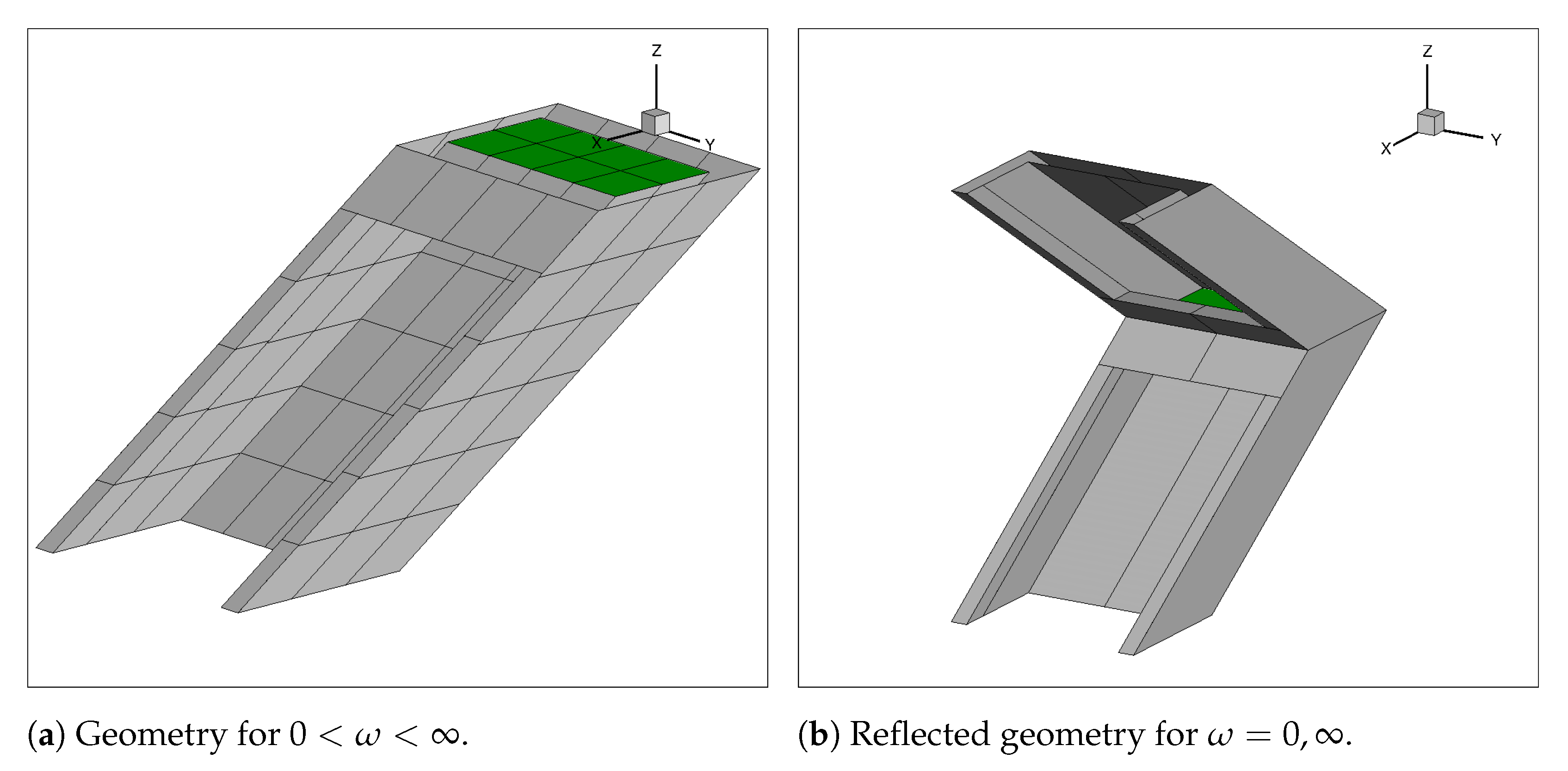
4.3. The Maynooth University/Dundalk IT Team

1-DOF state-space model: For the single-degree-of-freedom (1-DOF) case, two models were produced by the Maynooth University/Dundalk IT (MU/DkIT) Team. The first assumes incompressible flow through the orifice and uses Equation (17) to determine the mass flow rate of air between the chamber and atmosphere, while the second model assumes compressible flow through the orifice and uses Equation (18) to the same end. Both models use Equation (16) to model the pressure within the chamber, allowing a comparison to be made between the relative importance of the different compressible elements of the two models. Both 1-DOF models operate under the assumption that the water column acts in pumping mode only, referred to here as mode 7. The first sloshing mode, referred to as mode 8, results in an antisymmetric displacement of the free surface about a line parallel to the wave front running through the centroid of the free surface. Hence, there is no overall change in the air volume above the water column due to the sloshing mode, and it does not contribute to the power absorbed by the OWC; see Figure 13. The pumping mode is, therefore, the main ‘power’ mode of the OWC. The equation of motion of the water column in the KRISO device, for a single degree of freedom in the time domain, can be represented by a variation of Equation (11), also known as the modified Cummins equation [28]. The coupled equations Equations (11), (16), and (17) (or, in the case of the incompressible flow model, Equation (18)) are recast in state-space form. Such a form facilitates the replacement of the convolution term with a state-space approximation. The state variables are:

$${\left[\begin{array}{ccc}{r}_1& r_2& r_3\end{array}\right]}^T={\left[\begin{array}{ccc}{x}_7& {\dot{x}}_7& p\end{array}\right]}^T,$$

(20)

with the state-space model for this 1-DOF case documented in Reference [31], containing a parametric approximation for the convolution term, $con{v}_{77}={\displaystyle {\int }_0^t{K}_{77}(t-\tau ){\dot{x}}_7\left(\tau \right)d\tau }$, calculated through the FOAMM toolbox [40].

2-DOF state-space model: Following a similar procedure as for the 1-DOF models, two 2-DOF models were produced. The first 2-DOF model assumes the air flow across the orifice to be incompressible and uses Equation (17) to model the mass flow rate of air between the OWC chamber and atmosphere, while the second model assumes the air flow across the orifice to be compressible, but uses Equation (18) in place of Equation (17). Both 2-DOF models represent the motion of the water column in the KRISO using a modified version of Equation (11) for both mode 7 and mode 8, Equation (16) to model the pressure variation within the chamber, and either Equation (17) or Equation (18) to model the mass flow rate through the orifice, as appropriate. The systems of equations are then cast in state-space form. Based on the behavior of the WAMIT coefficients for the chamber, the following approximations are found to be justified:

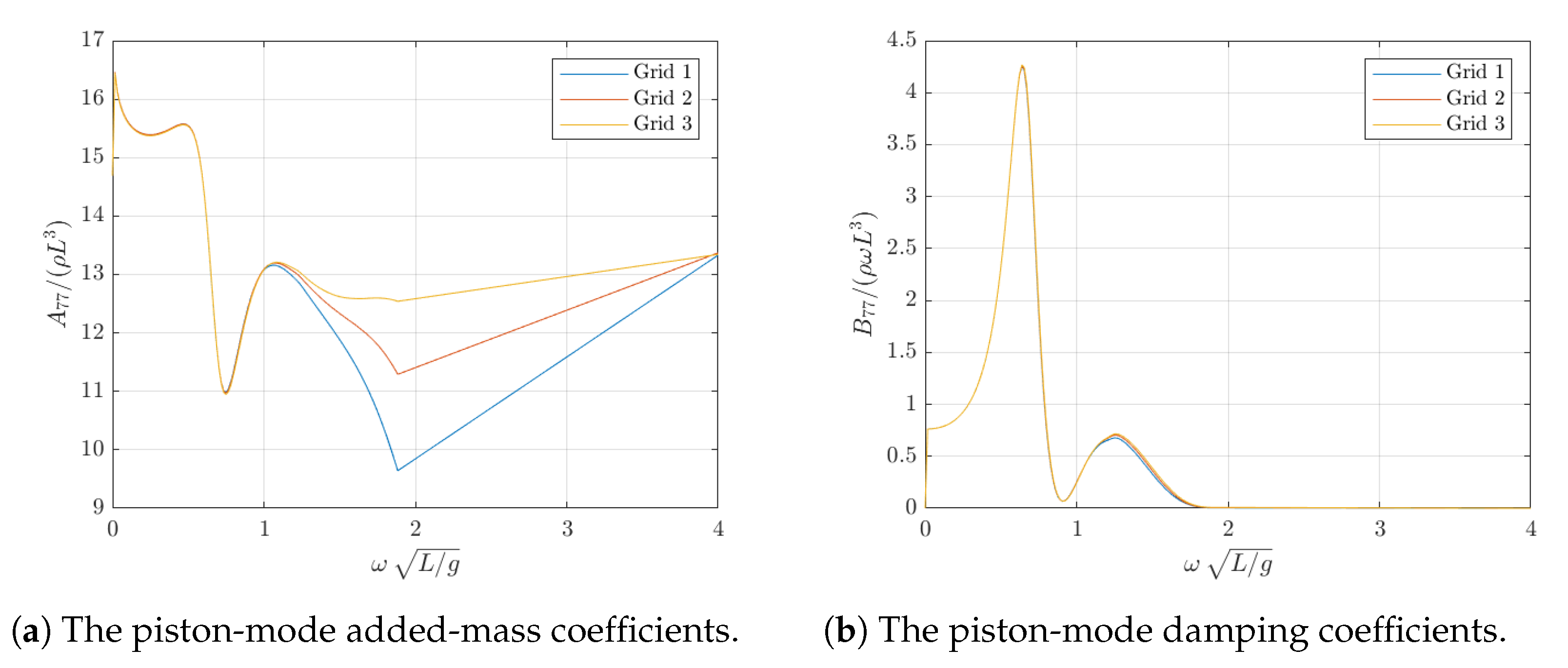
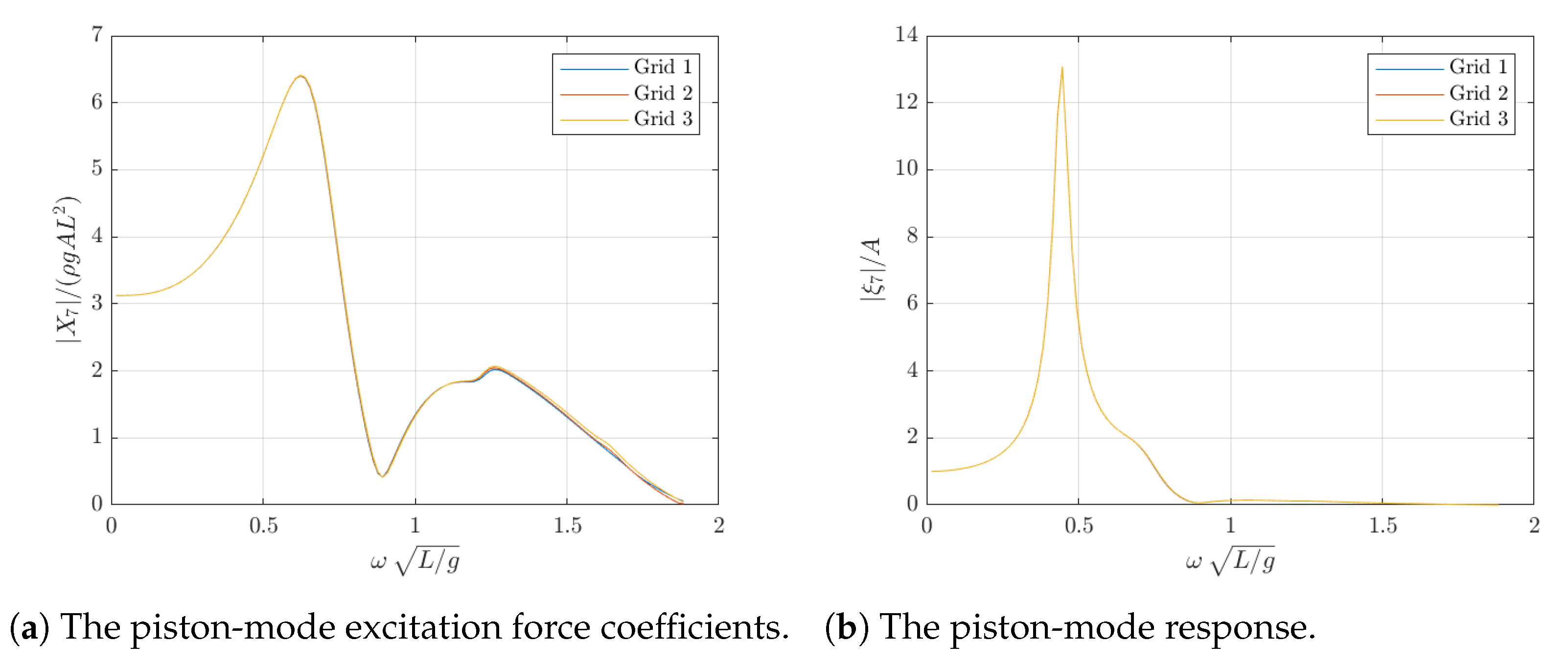
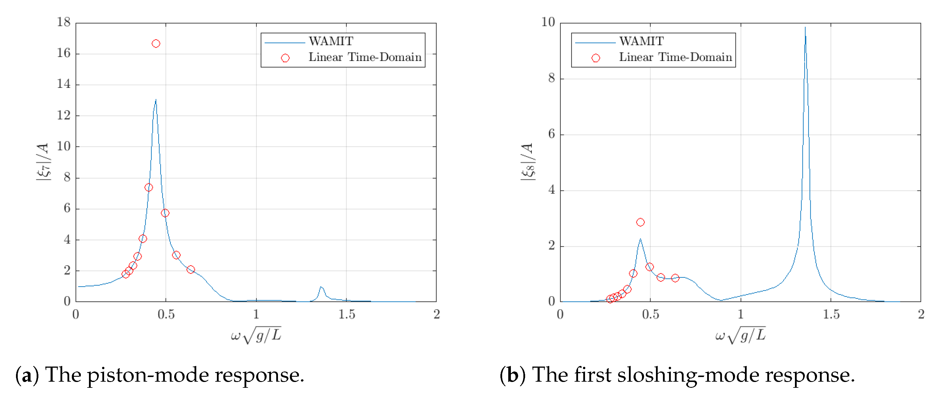
• The sloshing mode (mode 8) and the coupling modes (mode 78 and mode 87) are waveless (i.e., the convolution integrals for these modes can be set to zero).
• The coupling added masses, $a_{78}$ and $a_{87}$, are independent of frequency and equal to their infinite frequency values, $a_{78}^{\infty }$ and $a_{87}^{\infty }$, respectively.

The chosen state variables for the 2-DOF state-space model are:

$${\left[\begin{array}{ccccc}{r}_1& r_2& r_3& r_4& r_5\end{array}\right]}^T={\left[\begin{array}{ccccc}{x}_7& {\dot{x}}_7& x_8& {\dot{x}}_8& p\end{array}\right]}^T.$$

(21)

The state-space model can be represented as:

$$\begin{array}{c}\left(\begin{array}{c}{\dot{r}}_1\\ {\dot{r}}_2\\ {\dot{r}}_3\\ {\dot{r}}_4\\ {\dot{r}}_5\end{array}\right)=\left(\begin{array}{ccccc}0& 1& 0& 0& 0\\ -\alpha \left(\frac{c_{77}}{a_{77}^{\infty }}-\frac{a_{78}^{\infty }{c}_{87}}{a_{77}^{\infty }{a}_{88}^{\infty }}\right)& 0& -\alpha \left(\frac{c_{78}}{a_{77}^{\infty }}-\frac{a_{78}^{\infty }{c}_{88}}{a_{77}^{\infty }{a}_{88}^{\infty }}\right)& 0& -\alpha \left(\frac{A_c}{a_{77}^{\infty }}\right)\\ 0& 0& 0& 1& 0\\ -\alpha \left(\frac{c_{87}}{a_{88}^{\infty }}-\frac{a_{87}^{\infty }{c}_{77}}{a_{88}^{\infty }{a}_{77}^{\infty }}\right)& 0& -\alpha \left(\frac{c_{88}}{a_{88}^{\infty }}-\frac{a_{87}^{\infty }{c}_{78}}{a_{88}^{\infty }{a}_{77}^{\infty }}\right)& 0& \alpha \left(\frac{a_{87}^{\infty }{A}_c}{a_{88}^{\infty }{a}_{77}^{\infty }}\right)\\ 0& \frac{\gamma \left(r_5+p_a\right)}{[h_o-r_1]}& 0& 0& 0\end{array}\right)\left(\begin{array}{c}{r}_1\\ r_2\\ r_3\\ r_4\\ r_5\end{array}\right)\hfill \\ \hfill \hspace{1em}\hspace{1em} +\left(\begin{array}{ccc}0& 0& 0\\ \alpha \left(F_{7D}\left(t\right)-\frac{a_{78}^{\infty }{F}_{8D}\left(t\right)}{a_{88}^{\infty }}-con{v}_{77}\right)& 0& 0\\ 0& 0& 0\\ 0& \alpha \left(F_{8D}\left(t\right)-\frac{a_{87}^{\infty }{F}_{7D}\left(t\right)}{a_{77}^{\infty }}+\frac{a_{87}^{\infty }con{v}_{77}}{a_{77}^{\infty }}\right)& 0\\ 0& 0& \frac{c_s^2}{A_c\left[h_o-r_1\right]}\end{array}\right)\left(\begin{array}{c}\frac{1}{a_{77}^{\infty }}\\ \frac{1}{a_{88}^{\infty }}\\ \dot{m}\end{array}\right).\end{array}$$

(22)

Using the parametric approximation of $con{v}_{77}$ given by the matrices: $A_r$, $B_r$ and $C_r$, as described for example in Reference [40], the final state-space matrices for the 2-DOF model are

$$A_{2-dof}=\left[\begin{array}{cccccccc}& & & 0& & 0& 0& 0\\ & A_r& & ⋮& B_r& ⋮& ⋮& ⋮\\ & & & 0& & 0& 0& 0\\ 0& \cdots & 0& 0& 1& 0& 0& 0\\ & -\frac{\alpha C_r}{a_t}& & -\alpha \left[\frac{a_{88}^{\infty }{c}_{77}-a_{78}^{\infty }{c}_{87}}{a_t}\right]& 0& -\alpha \left[\frac{a_{88}^{\infty }{c}_{78}-a_{78}^{\infty }{c}_{88}}{a_t}\right]& 0& \frac{-\alpha a_{88}^{\infty }{A}_c}{a_t}\\ 0& \cdots & 0& 0& 0& 0& 1& 0\\ & -\frac{\alpha C_r}{a_t}& & -\alpha \left[\frac{a_{77}^{\infty }{c}_{87}-a_{87}^{\infty }{c}_{77}}{a_t}\right]& 0& -\alpha \left[\frac{a_{77}^{\infty }{c}_{88}-a_{87}^{\infty }{c}_{77}}{a_t}\right]& 0& \frac{-\alpha a_{87}^{\infty }{A}_c}{a_t}\\ 0& \cdots & 0& 0& \frac{\gamma (r_{5+n}+p_a)}{(h_o-r_{1+n})}& 0& 0& 0\end{array}\right],$$

$$B_{2-dof}=\left[\begin{array}{ccc}0& 0& 0\\ ⋮& ⋮& ⋮\\ 0& 0& 0\\ \alpha \left[F_{7D}\left(t\right)-\frac{a_{78}^{\infty }}{a_{88}^{\infty }}{F}_{8D}\left(t\right)\right]& 0& 0\\ 0& 0& 0\\ 0& \alpha \frac{a_{87}^{\infty }}{a_{77}^{\infty }}\left[\frac{a_{77}^{\infty }}{a_{87}^{\infty }}{F}_{8D}\left(t\right)-F_{7D}\left(t\right)\right]& 0\\ 0& 0& \frac{c_s^2}{A_c\left[h_o-r_{1+n}\right]}\end{array}\right],$$

where

$$\alpha =\frac{a_{77}^{\infty }{a}_{88}^{\infty }}{a_{77}^{\infty }{a}_{88}^{\infty }-a_{78}^{\infty }{a}_{87}^{\infty }},a_t=a_{77}^{\infty }{a}_{88}^{\infty }.$$

(23)

The 1-DOF and 2-DOF models are simulated in MATLAB as sets of ODEs in matrix form (state space), which are solved using the ‘ODE45’ solver based on an explicit Runge-Kutta integration formulation. The parametric approximations are used for both the radiation and excitation forces (Equation (12)) by using the methods described in References [40,41]. By generating both 1-DOF and 2-DOF models, the importance of the first sloshing mode on the performance of the model can be assessed.

4.4. The University of Plymouth Team

Incompressible CFD model: The open-source CFD code, OpenFOAM (version 4.1), is utilized in preliminary simulations of four of the physical wave tank test cases (Tests 107, 207, and 407). The code solves the unsteady, incompressible, RANS equations for two isothermal, immiscible fluids using a volume of fluid interface capturing scheme based on the multi-dimensional limiter for explicit solution (MULES) algorithm [42] and typical fluid properties (${\rho }_{water}$ = 1000 kg/m${}^3$, ${\rho }_{air}$ = 1.225 kg/m${}^3$). A variable time-stepping approach is used based on a maximum Courant number, $Co$, of 1.0. Pressure-velocity coupling is achieved via the Pressure Implicit with Splitting of Operators (PISO) algorithm [43] using one outer and three inner correctors. The k-$\omega$ SST (Shear Stress Transport) turbulence closure model is used with standard wall functions, for k, $\omega$, and ${\nu }_t$, on all walls (including the surface of the OWC and the tank floor).

The computational domain used in this study is similar in dimension to the physical wave tank, but due to the geometrical symmetry of the problem, only half the width of the physical problem is simulated. The computational domain is, therefore, 15 m wide, 6.2 m tall, and 59.5 m long. Wave generation and absorption is achieved, using the waves2Foam toolbox [44], via the second-order Stokes theory, expression-based boundary conditions for the phase fraction and velocity on the upstream and downstream boundaries and 5-m-long relaxation zones adjacent to both (Figure 18). A symmetry boundary condition is applied to the boundary coincident with the symmetry plane of the problem and a pressure inlet/outlet boundary condition is applied to the top boundary. All other boundaries are modeled using a no-slip condition.

A convergence study was undertaken in which four different meshes were considered using the same variable time-stepping approach and maximum Courant number, $Co$, of 1.0. These meshes had background mesh sizes of 0.38, 0.25, 0.16, and 0.11 m. The selected computational mesh, shown in Figure 18, has an average background cell side length of ≈0.25 m, with grading of the cells in the along-crest direction for $y>$ 3 m. The mesh has a number of regions of refinement, achieved using the quadtree refinement strategy and OpenFOAM’s snappyHexMesh utility; the mesh in the free-surface region and on the OWC surface is refined to level 2 (≈0.06 m), whereas the duct and orifice regions are refined to level 4 (≈0.015 m). The surfaces of the duct and orifice are also refined with four prismatic cell layers, with a first layer thickness of 1.6 mm and an expansion ratio of 2. The mesh has 1.03 million cells in total. The simulations were run on the University of Plymouth high-performance computing cluster. Each simulation took approximately 44 h to complete and used 700 cpu.hr.

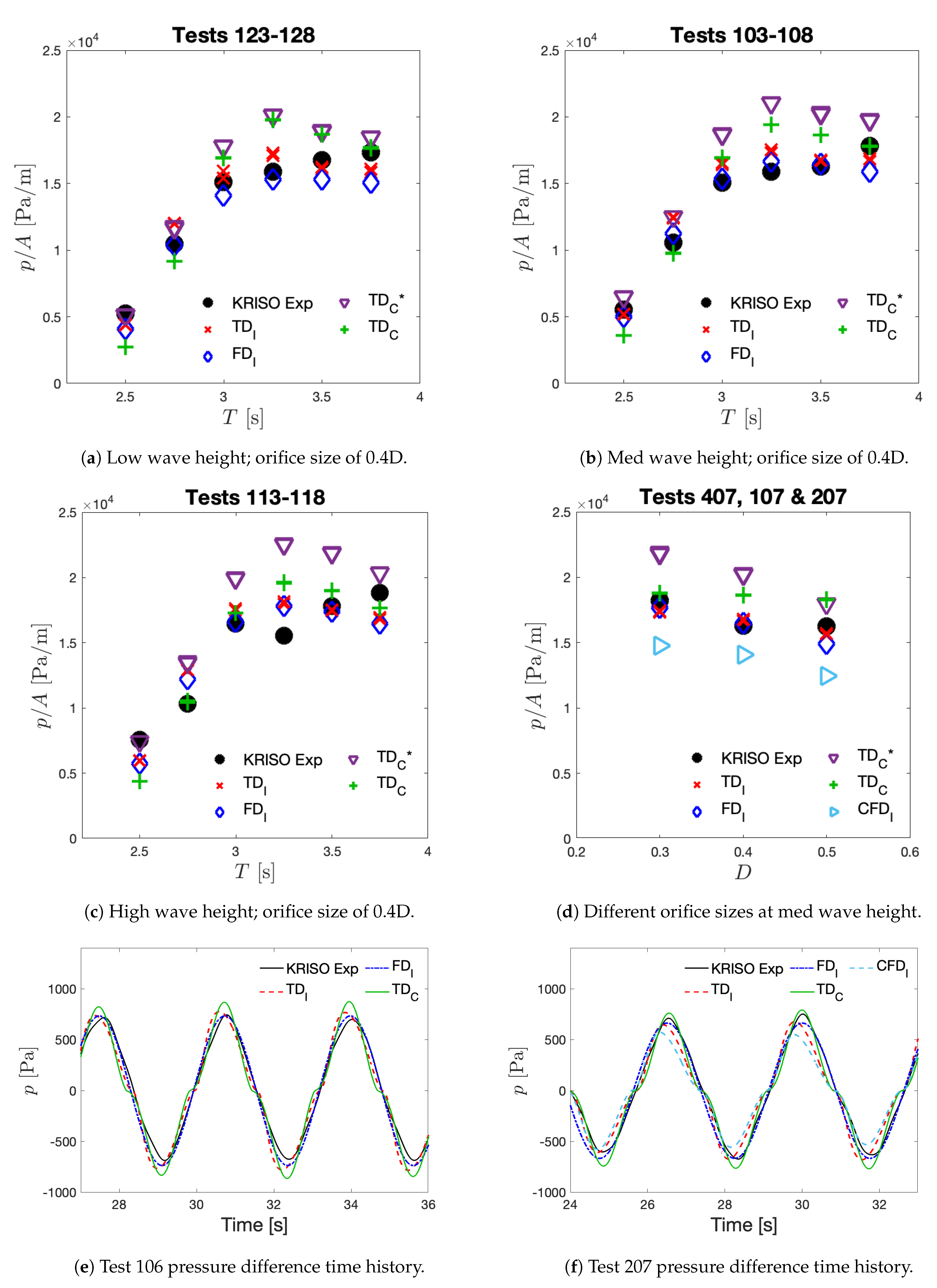
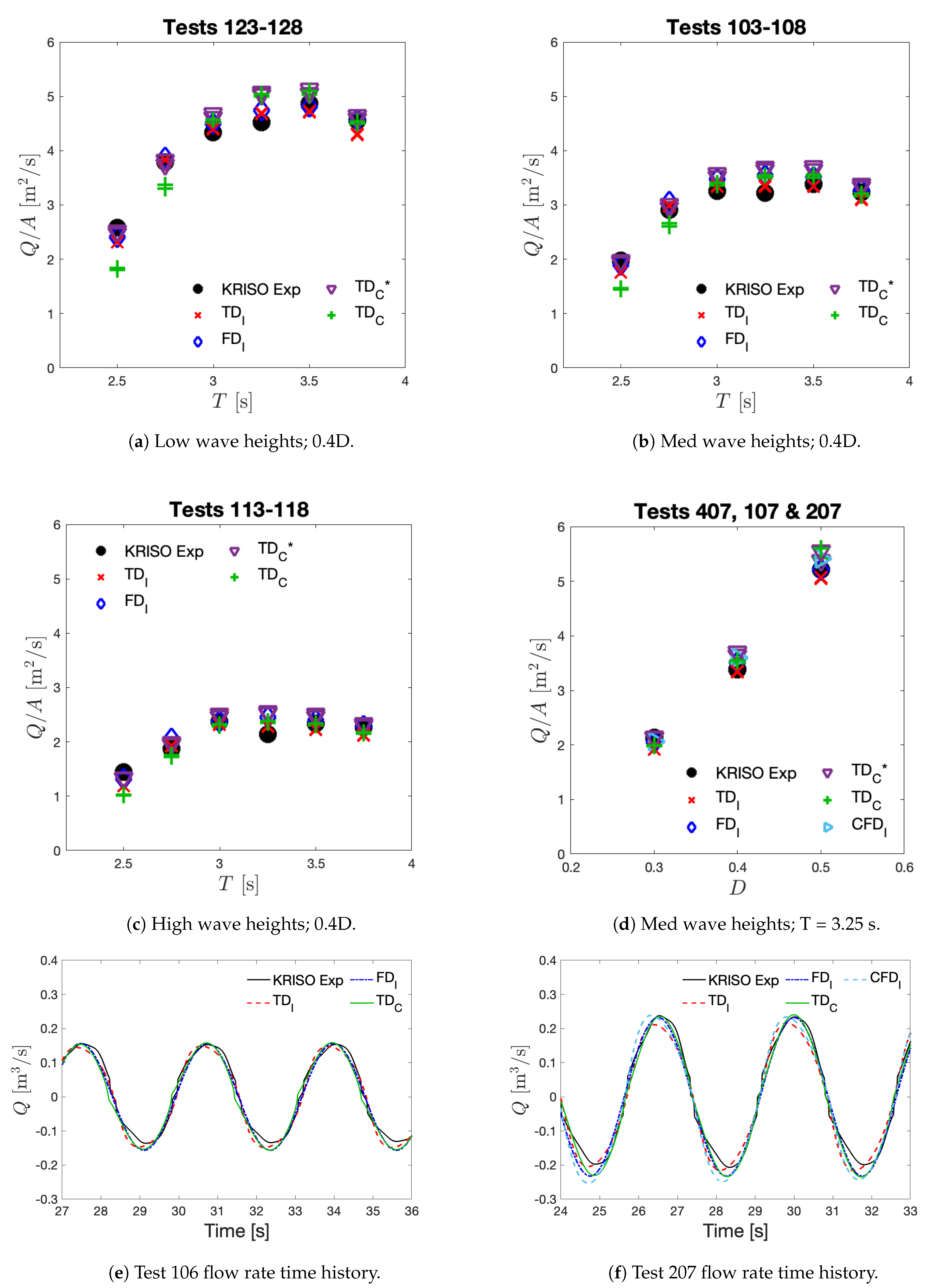
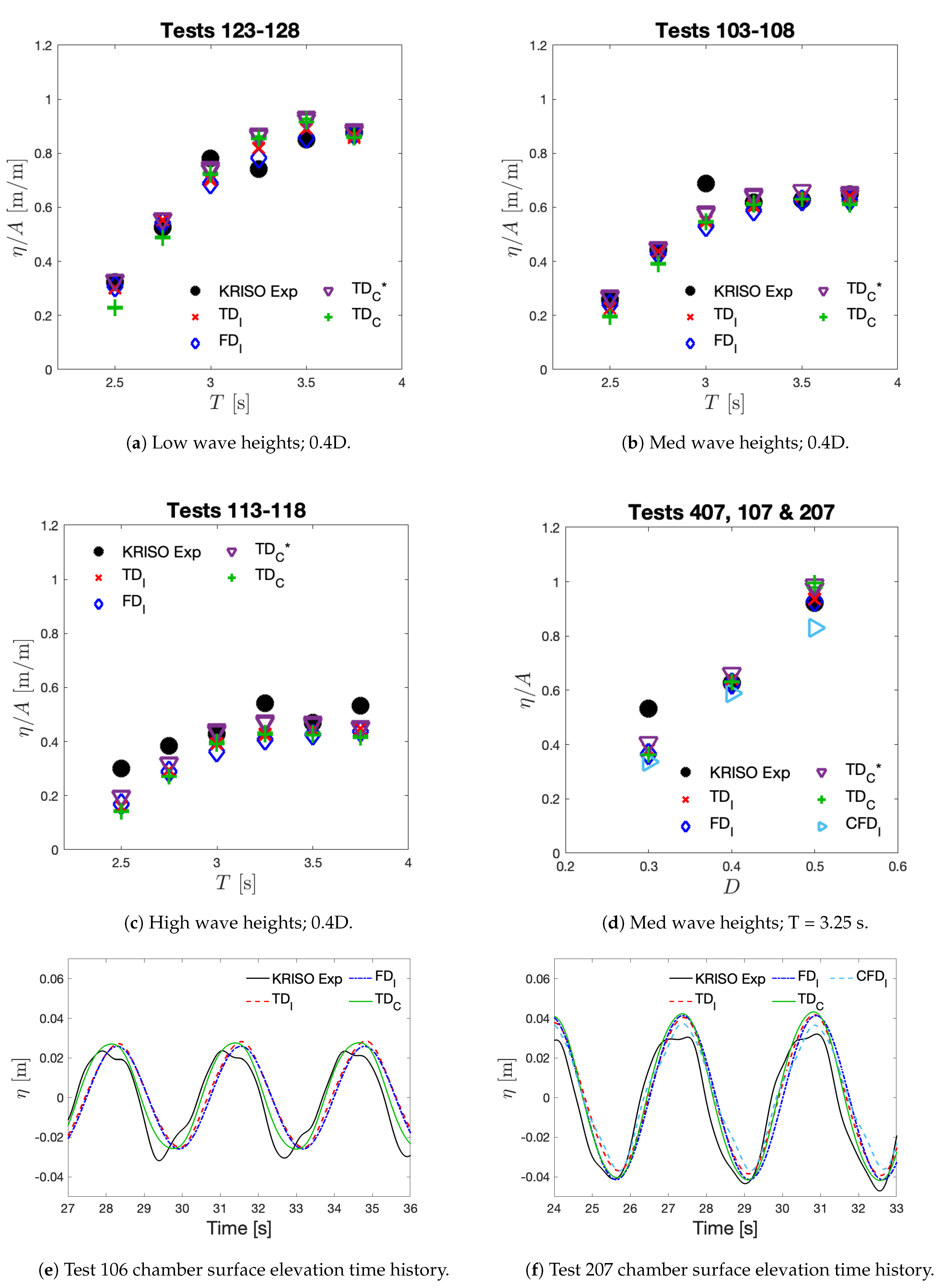
5. Comparison of Results

In this section, we compare all of the simulation results from the participants, including the pressure difference across the orifice plate, the flow rate, estimated power, and internal chamber surface elevation, to the KRISO experimental data. The undisturbed incident wave elevation signals obtained from the experimental measurements were directly applied in the time-domain solutions, but the frequency domain and CFD simulations used the specified wave height and wave period given in Table 1. The analysis section was selected to minimize the influence of wave reflections from the beach on the measured data, as shown in Figure 6.

The measured and simulated first-harmonic, time-averaged amplitudes of the internal chamber surface elevation, orifice flow rate, and orifice pressure difference are equal to half of the peak-to-trough values, which are calculated using the time history data over the three wave periods in each analysis section. The power is estimated based on the flow rate and the pressure difference across the orifice plate, and the average absorbed power over the analysis section can be calculated from

$$\begin{array}{c}\hfill \overline{P}=\frac{1}{T_r-T_s}{\int }_{T_s}^{T_r}Pdt,\end{array}$$

(24)

where $T_s$ and $T_r$ are the start and end times of the analysis section. For a fair comparison, the first-harmonic amplitude values and the averaged power output are scaled by the wave amplitude, which is equal to half of the wave height that was computed directly based on the peak and trough of the wave elevation time history from the analysis section.

5.1. Potential Flow Solutions

In this section, we focus mainly on the potential flow model results, but also include one set of CFD solutions provided by the University of Plymouth team. The pressure difference is created by the presence of the orifice plate. In the potential flow model, this is the pressure difference between the internal chamber and the atmosphere, while in the experiments and the CFD simulations, it is the pressure difference across the orifice plate, as shown in Figure 5. The measured and computed pressure difference across the orifice plate are plotted in Figure 19. We note that the incompressible-flow, weakly-nonlinear, time-domain solutions computed by the three teams (DTU, NREL, MU/DkIT) all gave results that are nearly graphically identical, so only one curve/point is visible for this method. This confirms that the different numerical implementations of this formulation are all reasonably converged and consistent. In general, there are only small differences between the incompressible-flow, time- and frequency-domain solutions, indicating a consistency between the two evaluations of the weakly-nonlinear pressure term. The solutions from the compressible models give slightly higher peaks than those predicted by the incompressible methods. For the compressible-flow, air-chamber models of the MU/DkIT team, very small differences are found between the compressible- and incompressible-flow models for the flow through the orifice plate; therefore, only the 1-DOF and 2-DOF fully compressible-flow values are shown, and only the 2-DOF fully compressible-flow solutions are presented in the time history plots. It is notable that the quadratic damping term in the time-domain potential flow models results in a nonlinear behavior of the signal near the zero-crossing, in the simulated time history. However, this nonlinear behavior was not observed in the KRISO experimental measurements.

Figure 20 plots the measured and simulated flow rate from the potential flow solutions and the KRISO experimental data. In the experiments, by comparing to the time derivative of the internal chamber surface elevation, it was determined that it is more accurate to estimate the flow rate by taking the value from the upper gauge (HWA1) for the outflow and from the lower gauge (HWA2) for the inflow, as mentioned in Section 2.1. For consistency, the flow rate in the CFD simulations was computed using the same upper/lower gauge approach that was used in the experiments. In the potential flow models, the simulated flow rate depends on the coefficient $C_d$, appearing in the pressure-flux relation of Equation (6). Based on the pressure difference and the ’outflow’ flow rate obtained from the experimental data, the value of $C_d$ was estimated to be 0.8271. Since the $C_d$ value was tuned based on the experimental measurements, all codes with different modeling approaches generally agree with the estimated flow rate from the KRISO data. Because the $C_d$ value was estimated using only the outflow, the potential flow solutions have a better agreement with the KRISO data for the outflow cycle, when the flow rate is positive.

Figure 21 plots the measured and simulated internal surface elevations at the center of the chamber. The predicted internal chamber surface elevation amplitude is similar to the measurements, except for the high wave-height cases, where all the potential flow models underestimate the surface elevation. However, the nonlinear behavior of chamber surface elevation at the peaks, which is apparent in the experiments, is not captured by any of the potential flow models. In addition, a phase shift is observed between the compressible and incompressible solutions, in particular for Test 106. This is one expected effect of the compressibility of the air phase in the chamber, since it acts like a mechanical spring which is in phase with the chamber motion rather than the chamber velocity. This introduces a phase shift compared to the incompressible model where the pressure and the chamber surface velocity are exactly in phase.

Figure 22 shows the average absorbed power, which is calculated from the measured and simulated data. In the time history plots, the high and low peaks observed in the measured data are mainly caused by the difference of flow rate between the outflow and inflow, which is not reproduced by the potential flow models because the same $C_d$ value is used for both the outflow and inflow in the simulations. Thus, it also follows that the estimated power outputs from the potential flow models agree better with the experiments for the outflow cycle.

To summarize these results, we calculated the maximum percentage difference between the KRISO measurements and the solutions from the potential flow models. The percentage difference is determined based on the maximum value of the pressure difference, chamber surface elevation, flow rate, and averaged power from the test cases, and the results are listed in

Table 3. A summary of the difference between the measured and potential flow solutions.

	Maximum Percentage Difference from the KRISO Exp
Model	Pressure Difference	Chamber Surface Elevation	Flow Rate	Power
TD${}_{\mathrm{I}}$	14%	16%	5%	15%
FD${}_{\mathrm{I}}$	13%	18%	6%	10%
TD${}_{\mathrm{C}}$	21%	18%	15%	17%
TD${}_{\mathrm{C}}$	37%	14%	11%	17%

. Overall, the differences between the potential flow model solutions and experimental data are within 21%, except for the 1-DOF model, which only considers the piston mode for the chamber surface motion. Although all of the results show a similar trend, with relatively small differences in the predicted first-harmonic amplitudes, only the compressible-flow model is able to capture the small phase shift in the chamber surface elevation relative to the pressure.

5.2. CFD Simulations

As discussed in Section 2.1 and Section 5.1, the expected variation of air density due to air compressibility inside the chamber is small for these experiments. However, while the influence of air compressibility on the flow through the orifice plate was found to be very small, a small but significant phase shift between the chamber surface elevation and the pressure was accurately captured by the compressible model for the air volume in the chamber. To further investigate the significance of nonlinearity in the system, verify the numerical solutions and better understand the effect of air compressibility, both incompressible and compressible CFD simulations were performed for Test 106. This case was chosen because it is the largest-amplitude case which is still free of reflection effects from the beach.

The measured and simulated pressure differences across the orifice plate for Test 106 are plotted in Figure 23. In addition to the CFD solutions, the result from the incompressible and compressible potential flow time-domain models (NREL_WECSim and MU’s 2–DOF), with both $C_d=0.65$ and $C_d=0.8271$, are also included. The quadratic nonlinearity of the signal near the zero-crossing observed in the potential flow model is perfectly captured in the incompressible CFD simulation. However, this nonlinear behavior is not observed in the compressible CFD simulation, and the effect of air compressibility then seems to explain why this nonlinear behavior near the zero crossing is not observed in the experimental data. The compressible CFD simulation also captures the small phase shift of the peaks observed in the KRISO experiments. In general, the effect of air compressibility has a small influence on the predicted pressure difference. The amplitude of the pressure difference across the orifice obtained from the compressible CFD simulation is slightly higher than that predicted by the incompressible CFD simulation, which is consistent with the trend shown by the potential flow calculations.

On the other hand, estimation of the flow rate is the primary source of uncertainty in the experiments. To better understand this, we compare the measured flow rate to that obtained from the CFD simulations and the potential flow models. The results are plotted in Figure 24. Here, two different approaches are used to estimate the experimental flow rate. One is based on the previously described upper/lower air velocity gauge approach, and the other is obtained by taking the average of the two measurements. In both the incompressible and compressible CFD simulations, we directly compute the flow rate by integrating the flow velocity across a surface plane at the orifice. The predicted flow rate from the CFD simulations is closer to the experimental data using the average value from the two velocity gauges and the potential flow solution when $C_d=0.65$ is used. $C_d$ represents a time-averaged value, which is calculated using the correlation between the pressure difference and flow rate, as described in Section 2.1, and the time history data of the last three wave periods from the compressible CFD simulation. For the effect of air compressibility, which is similar to what we have found for the pressure difference, the peaks are slightly shifted, and the flow rate magnitude obtained using the compressible CFD simulation is slightly higher than the prediction from the incompressible CFD simulation.

To better quantify the flow rate calculation uncertainty, we compare the computed flow rate from the compressible CFD simulations using different methods including: the upper/lower gauge approach; the average value from the upper and lower gauges; the velocity at the center of the orifice; and, finally, integration of the flow velocity over a surface plane inside the duct or at the orifice, which should give the true flow rate. This comparison is presented in Figure 25, and the solution from the incompressible CFD simulation is also included for reference. Based on the results from the CFD simulations, the flow rate is overestimated when using the upper/lower gauge approach. To further investigate the differences, we plot the velocity magnitude at the upper (HWA1) and lower (HWA2) gauges in Figure 26. The CFD solutions are close to the measurements. However, the measured downstream velocity magnitude is smaller than the CFD solutions, and the measured upstream velocity magnitude is larger than the CFD results, particularly for HWA2. Moreover, the measured velocity magnitude has a higher peak value for the outflow than the inflow, whereas the calculated values are nearly the same. In addition, as shown in Figure 26, the calculations predict that the velocity near the orifice is very sensitive to the vertical location, and varies almost linearly. This probably explains why the estimated flow rate is smaller if calculated from the average value of the two velocity gauges and why there is a significant difference between the outflow flow rate and the inflow flow rate.

Typically, compressible flow is considered as being relevant for a flow velocity with a Mach number greater than 0.3. For Test 106, the Mach number is about 0.1, using the maximum flow velocity near the orifice from the CFD simulations. Based on the estimated Mach number, and the calculated air density variation, as described in Section 2.1, we initially assumed that air compressibility effects would be insignificant for these experiments. This is the case for the pressure difference and the flow rate. However, the effect of air compressibility has a significant influence on the chamber surface elevation. A comparison of the internal chamber surface elevation at the center of the chamber (wave gauge #5), using both the compressible and incompressible CFD simulations, is shown in Figure 27. The predicted chamber elevation from compressible CFD is slightly smaller but captures the nonlinear time history profile fairly well. There is a significant difference between the solutions from compressible and incompressible CFD simulations. The air compressibility also introduces a phase shift in the chamber surface elevation. In addition, like the measured data, the compressible flow CFD results show a larger time derivative near the zero-crossing compared to the incompressible CFD solution, which is the main reason why the estimated value for the peak flow rate is larger when using the chamber wave elevation for the calculation.

Figure 28 shows a comparison of the measured and simulated power outputs, which are directly calculated based on the pressure difference (Figure 23) and the flow rate (Figure 25). Note that the experimental pressure difference is obtained from direct measurement, regardless of how the flow rate is estimated. Different ways of estimating the flow rate result in different power estimates. For Test 106, the estimated power from the compressible CFD simulation is about 13% higher than the prediction from the incompressible CFD simulation, and the estimated power from the experiment using the upper/lower gauge flow rate calculation approach is about 15% higher than the estimated power from the compressible CFD simulation. The latter is essential because the time derivative of the chamber wave elevation is often used to estimate the flow rate, when the flow velocity through the orifice is not available. Focusing on the compressible models and the measurements here, we can see the sensitivity of the power estimate to the assumed flow-rate through the orifice and the chosen value of $C_d$, illustrating the importance of getting these values accurately from the experimental conditions. The results from this study indicate that this approach can be misleading when the effect of air compressibility is non-negligible. It is anticipated that, for smaller orifice cases, the difference is most likely to be larger because of the increase of flow velocity and a larger Mach number, where the effect of air compressibility becomes even more important.

6. Conclusions

A set of relatively large-scale measurements for a breakwater-mounted OWC chamber has been carefully analyzed and compared with numerical predictions based on weakly-nonlinear time- and frequency-domain potential flow methods, and CFD. The air phase has been modeled using both incompressible- and compressible-flow models. The effects of air compressibility are found to be small for the pressure difference across the orifice plate, but they produce significant nonlinear effects and a significant phase shift of the internal chamber surface motion. All models capture the time-averaged quantities well, but only the compressible CFD model is able to accurately reproduce the detailed responses.

This study highlights a number of important guidelines for the production of benchmark experimental data suitable for comparing the relative accuracy of different levels of numerical modeling. Ideally, benchmark data should include repetition of each case, so that the uncertainty of all measured quantities can be quantified to produce reliable confidence bounds. This begins with the undisturbed wave conditions in the basin without the structure in place, and then all measured quantities with the structure in place. Once the realization uncertainties are established, they can be combined with measurement errors to establish 95% confidence intervals, which then allow the data to be used to precisely evaluate the accuracy of the numerical models. For OWC-type devices, special care needs to be taken to determine the pressure-flux relation for the flow through the orifice plate, or the model turbine, which is used to extract power from the system. Ideally, the pressure difference should be measured between the chamber and the atmosphere to avoid local effects near the orifice/turbine.

Finally, we have illustrated a simple and accurate method for using state-of-the-art BEM solutions to accurately determine the infinite frequency added mass for OWC chambers. This method should replace ad-hoc approaches which are commonly applied to address this problem.

References

1. Dallman, A.; Jenne, D.S.; Neary, V.; Driscoll, F.; Thresher, R.; Gunawan, G. Evaluation of performance metrics for the Wave Energy Prize converters tested at 1/20th scale. Renew. Sustain. Energy Rev. 2018, 98, 79–91. [Google Scholar] [CrossRef]
2. Wendt, F.; Nielsen, K.; Yu, Y.H.; Bingham, H.B.; Eskilsson, C.; Kramer, M.; Babarit, A.; Bunnik, T. Ocean energy systems wave energy modelling task: Modelling, verification and validation of wave energy converters. J. Mar. Sci. Eng. 2019, 7, 379. [Google Scholar] [CrossRef] [Green Version]
3. Heath, T. A review of oscillating water columns. Philos. Trans. Roy. Soc. Lond. A 2012, 370, 235–245. [Google Scholar] [CrossRef] [Green Version]
4. Falcão, A.F.O.; Henriques, J.C.C. Model-prototype similarity of oscillating-water-column wave energy converters. Int. J. Mar. Energy 2014, 6, 18–34. [Google Scholar] [CrossRef]
5. Vicinanza, D.; Di Lauro, E.; Contestabile, P.; Gisonni, C.; Lara, J.L.; Losada, I.J. Review of innovative harbor breakwaters for wave-energy conversion. J. Waterway Port Coastal Ocean Eng. 2019, 145, 1–18. [Google Scholar] [CrossRef]
6. Babarit, A. Wave Energy Conversion. Resource, Technology and Performance; ISTE Press Ltd.: London, UK, 2018. [Google Scholar] [CrossRef]
7. Cruz, J. Ocean Wave Energy. Current Status and Future Perspectives; Springer: Berlin/Heidelberg, Germany, 2008. [Google Scholar]
8. Yu, Y.H.; Lawson, M.; Ruehl, K.; Michelen, C. Development and demonstration of the WEC-Sim wave energy converter simulation tool. In Proceedings of the 2nd Marine Energy Technology Symposium, U.S. Department of Energy, Seattle, WA, USA, 15–18 April 2014. [Google Scholar]
9. Papillon, L.; Costello, R.; Ringwood, J.V. Boundary element and integral methods in potential flow theory: A review with a focus on wave energy applications. J. Ocean. Eng. Mar. Energy 2020, 6, 303–337. [Google Scholar] [CrossRef]
10. Windt, C.; Davidson, J.; Ringwood, J.V. High-fidelity numerical modelling of ocean wave energy systems: A review of computational fluid dynamics-based numerical wave tanks. Renew. Sustain. Energy Rev. 2018, 93, 610–630. [Google Scholar] [CrossRef] [Green Version]
11. Bingham, H.B.; Ducasse, D.; Nielsen, K.; Read, R. Hydrodynamic Analysis of Oscillating Water Column, Wave Energy Devices. J. Ocean Eng. Mar. Energy 2015, 1, 405–419. [Google Scholar] [CrossRef] [Green Version]
12. WAMIT. WAMIT; User Manual, Version 7.0; WAMIT, Inc.: Chestnut Hill, MA, USA, 2008–2012; Available online: http://www.wamit.com (accessed on 17 March 2021).
13. Sheng, W.; Alcom, R.; Lewis, A. Assessment of primary energy conversions of oscillating water columns. I. Hydrodynamic analysis. J. Renew. Sustain. Energy 2014, 6, 053113. [Google Scholar] [CrossRef] [Green Version]
14. Luczko, E.; Robertson, B.; Bailey, H.; Hiles, C.; Buckham, B. Representing non-linear wave energy converters in coastal wave models. Renew. Energy 2018, 118, 376–385. [Google Scholar] [CrossRef]
15. Henriques, J.C.C.; Sheng, W.; Falcão, A.F.O.; Gato, L.M.C. A comparison of biradial and Wells air turbines on the Mutriku breakwater OWC wave power plant. In Proceedings of the 36th International Conference on Ocean, Offshore and Arctic Engineering, Trondheim, Norway, 25–30 June 2017. [Google Scholar]
16. Henriques, J.C.C.; Gomes, R.P.F.; Gato, L.M.C.; Robles, E.; Ceballos, S. Testing and control of a power take-off system for an oscillating-water-column wave energy converter. Renew. Energy 2016, 85, 714–724. [Google Scholar] [CrossRef]
17. Park, S.; Kim, K.H.; Nam, B.W.; Kim, J.S.; Hong, K. Experimental and numerical analysis of performance of oscillating water column wave energy converter applicable to breakwaters. In Proceedings of the 38th International Conference on Ocean, Offshore and Arctic Engineering, Glasgow, Scotland, 9–14 June 2019. [Google Scholar]
18. Fenton, J.D. Nonlinear wave theories. In The Sea; Le Mehaute, B., Hanes, D.M., Eds.; John Wiley & Sons.: Hoboken, NJ, USA, 1990; pp. 3–25. [Google Scholar]
19. Bullen, P.R.; Cheeseman, D.J.; Hussain, L.A.; Ruffell, A.E. The determination of pipe contraction pressure loss coeffients for incompressible turbulent flow. Heat Fluid Flow 1987, 8, 111–118. [Google Scholar] [CrossRef]
20. Newman, J.N. Marine Hydrodynamics; The MIT Press: Cambridge, MA, USA, 1977. [Google Scholar]
21. Falnes, J. Ocean Waves and Oscillating Systems; Cambridge University Press: Cambridge, UK, 2002. [Google Scholar]
22. Faltinsen, O.M. Sea Loads on Ships and Offshore Structures; Cambridge University Press: Cambridge, UK, 1990. [Google Scholar]
23. Evans, D.V. Wave-power absoption by systems of oscillating surface pressure distributions. J. Fluid Mech. 1982, 114, 481–499. [Google Scholar] [CrossRef]
24. Lee, C.H.; Nielsen, F.G. Analysis of Oscillating Water Column Device Using a Panel Method. 1996. Available online: http://www.iwwwfb.org (accessed on 17 March 2021).
25. Lee, C.H.; Newman, J.N.; Nielsen, F.G. Wave Interactions with an Oscillating Water Column. In Proceedings of the 6th International Offshore and Polar Engineering Conference, Los Angeles, CA, USA, 26–31 May 1996. [Google Scholar]
26. Newman, J.N.; Lee, C.H. WAMIT: A Radiation-Diffraction Panel Program for Wave-Body Interactions. 2020. Available online: http://www.wamit.com (accessed on 17 March 2021).
27. Newman, J.N. Wave effects on deformable bodies. Appl. Ocean. Res. 1994, 16, 47–59. [Google Scholar] [CrossRef]
28. Cummins, W.E. The impulse response function and ship motions. Schiffstecknik 1962, 9, 101–109. [Google Scholar]
29. Kelly, T.; Campbell, J.; Dooley, T.; Ringwood, J. Modelling and results for an array of 32 oscillating water columns. In Proceedings of the EWTEC 2013, Aalborg, DK, 2–5 September 2013. [Google Scholar]
30. Sheng, W.; Alcorn, R.; Lewis, A. On thermodynamics in the primary power conversion of oscillating water column wave energy converters. J. Renew. Sustain. Energy 2013, 5, 023105. [Google Scholar] [CrossRef] [Green Version]
31. Kelly, T. Experimental and Numerical Modelling of a Multiple Oscillating Water Column Structure. Ph.D. Thesis, Maynooth University, Maynooth, Ireland, 2018. [Google Scholar]
32. Cunningham, R. Orifice Meters with Supercritical Compressible Flow. Trans. ASME 1951, 73, 625–638. [Google Scholar]
33. Newman, J.N. (Woods Hole, MA, USA). Personal communication. 2018.
34. Davidson, J.; Costello, R. Efficient Nonlinear Hydrodynamic Models for Wave Energy Converter Design—A Scoping Study. J. Mar. Sci. Eng. 2020, 8, 35. [Google Scholar] [CrossRef] [Green Version]
35. Roenby, J.; Bredmose, H.; Jasak, H. A computational method for sharp interface advection. R. Soc. Open Sci. 2016, 3, 160405. [Google Scholar] [CrossRef] [Green Version]
36. Bingham, H.B.; Read, R. DTUMotionSimulator: A Matlab Package for Simulating Linear or Weakly Nonlinear Response of a Floating Structure to Ocean Waves. 2020. Available online: https://gitlab.gbar.dtu.dk/oceanwave3d/DTUMotionSimulator (accessed on 17 March 2021).
37. Bingham, H.B. A hybrid Boussinesq-panel method for predicting the motions of a moored ship. Coast. Eng. 2000, 40, 21–38. [Google Scholar] [CrossRef]
38. WEC-Sim (Wave Energy Converter SIMulator). Available online: https://wec-sim.github.io/WEC-Sim/ (accessed on 17 March 2021).
39. Guo, Y.; Yu, Y.H.; van Rij, J.; Tom, N. Inclusion of Structural Flexibility in Design Load Analysis for Wave Energy Converters. In Proceedings of the 12th European Wave and Tidal Energy Conference, EWTEC, Cork, Ireland, 27 August–1 September 2017. [Google Scholar]
40. Faedo, N.; Pena-Sanchez, Y.; Ringwood, J.V. Finite-Order Hydrodynamic Model Determination Using Moment-Matching. Ocean. Eng. 2018, 163, 251–263. [Google Scholar] [CrossRef] [Green Version]
41. Guo, B.; Patton, R.J.; Jin, S.; Lan, J. Numerical and experimental studies of excitation force approximation for wave energy conversion. Renew. Energy 2018, 125, 877–889. [Google Scholar] [CrossRef]
42. Rusche, H. Computational Fluid Dynamics of Dispersed Two-Phase Flows at High Phase Fractions. Ph.D. Thesis, Imperial College of Science, Technology & Medicine, London, UK, 2002. [Google Scholar]
43. Issa, R.I. Solution of the implicitly discretised fluid flow equations by operator-splitting. J. Comput. Phys. 1986, 62, 40–65. [Google Scholar] [CrossRef]
44. Jacobsen, N.G.; Fuhrman, D.R.; Fredsøe, J. A wave generation toolbox for the open-source CFD library: OpenFOAM®. Int. J. Numer. Methods Fluids 2012, 70, 1073–1088. [Google Scholar] [CrossRef]
Figure 1. The Korea Research Institute of Ships and Ocean Engineering (KRISO) wave basin where the tests were performed.
Energies 14 01718 g001
Figure 2. The location of the wave probes in the basin.
Energies 14 01718 g002
Figure 3. The test wave conditions in terms of nonlinearity, H / λ , relative water depth, k h , and the maximum possible wave steepness, H m a x / λ , as given by Reference [18].
Energies 14 01718 g003
Figure 4. The particulars of the chamber model used in the experiment: (a) chamber geometry and dimensions; (b) duct dimensions; and (c) the installed model in the basin.
Energies 14 01718 g004
Figure 5. The locations of the internal chamber wave gauges (indicated by WG), along with the pressure sensors (indicated by DPT) and hot wire anemometer probes (indicated by HWA) inside the duct.
Energies 14 01718 g005
Figure 6. Examples of the incident wave elevations at the chamber, showing the target wave amplitude and the chosen section used for analysis. (a) The time for the group velocity to travel from the chamber to the beach and back again (74 m); (b) Test 106; (c) Test 107; and (d) Test 108.
Energies 14 01718 g006
Figure 7. Measured chamber motions and pressure difference across the orifice plate for Test 106.
Energies 14 01718 g007
Figure 8. The variation in air density inside the chamber for Test 118, based on Equation (2).
Energies 14 01718 g008
Figure 9. Control volumes for estimating the pressure drop associated with flow from the chamber to the duct and through the orifice plate.
Energies 14 01718 g009
Figure 10. Estimates of the measured volume flux for two cases based on measurements of the mean chamber surface elevation (from η ¯ ), the pressure and Equation (6) (from p ¯ ) and the air flow velocity through the orifice (from u ¯ a ). A positive flow rate represents air flowing from the chamber to the atmosphere.
Energies 14 01718 g010
Figure 11. Estimates of the measured power absorption computed from the product of the measured pressure and each of the flux estimates shown in Figure 10, i.e., based on each of the three measured quantities: η ¯ , p ¯ , and u ¯ a . The horizontal lines indicate the mean power absorption per wave cycle.
Energies 14 01718 g011
Figure 12. The WAMIT geometries used to compute the coefficients. In (a), the z = 0 plane coincides with the green internal chamber surface. In (b), the z = 0 plane lies at the top of the reflected geometry and the green internal chamber surface becomes a dipole patch at the level z = −h in a fluid of depth 2h.
Energies 14 01718 g012
Figure 13. Illustration of the two-mode decomposition of the chamber surface motion using linear theory.
Energies 14 01718 g013
Figure 14. Convergence of the WAMIT piston-mode added-mass and damping coefficients for three grid resolutions.
Energies 14 01718 g014
Figure 15. Convergence of the WAMIT piston-mode excitation forces and motion response for three grid resolutions.
Energies 14 01718 g015
Figure 16. Comparison between the time- and frequency-domain free response of the chambers.
Energies 14 01718 g016
Figure 17. STAR-CCM+ computational domain and grid refinement regions for the wave regimes, the duct, and the orifice.
Energies 14 01718 g017
Figure 18. OpenFOAM computational domain and grid refinement regions for the wave regimes, the duct, and the orifice.
Energies 14 01718 g018
Figure 19. Comparison of the pressure difference: (ac) cases with low, med and high wave heights and an orifice plate size of 0.4D; (d) tests with orifice plate sizes corresponding to 0.3D, 0.4D, and 0.5D at med wave height; and (e,f) pressure difference time history for Tests 106 and 207. Superscript * indicates the 1-DOF (Degrees of freedom) model, and all the other potential flow models are 2-DOF, using both modes to approximate the internal surface motion. Subscript I and C indicate the incompressible and compressible flow models, respectively.
Energies 14 01718 g019
Figure 20. Comparison of the flow rate: (ac) cases with low, med and high wave heights and an orifice plate size of 0.4D; (d) tests with orifice plate sizes corresponding to 0.3D, 0.4D, and 0.5D in med wave height; and (e,f) flow rate time history for Tests 106 and 207.
Energies 14 01718 g020
Figure 21. Comparison of the internal chamber surface: (ac) cases with low, med and high wave heights and an orifice plate size of 0.4D; (d) tests with orifice plate sizes corresponding to 0.3D, 0.4D, and 0.5D in med wave height; and (e,f) chamber surface elevation time history for Tests 106 and 207.
Energies 14 01718 g021
Figure 22. Comparison of the averaged power output: (ac) cases with low, med and high wave heights and an orifice plate size of 0.4D; (d) tests with orifice plate sizes corresponding to 0.3D, 0.4D, and 0.5D in med wave height; and (e,f) power output time history for Tests 106 and 207.
Energies 14 01718 g022
Figure 23. Comparison of the measured, Computational Fluid Dynamics (CFD), and potential flow pressure difference with a zoom at the peak and near the zero crossing for Test 106.
Energies 14 01718 g023
Figure 24. Comparison of the measured, CFD, and potential flow flux and zooms at the peak and near the zero crossing for Test 106, comparing the use of the upper/lower gauge approach and the average of the two gauges for the experimental data.
Energies 14 01718 g024
Figure 25. (a) Comparison of the flow rate magnitude using different methods for Test 106; (b) flow rate at different surface planes from the incompressible CFD simulation; and (c) the orientation of those surface planes inside the duct.
Energies 14 01718 g025
Figure 26. (a) Comparison of the measured and CFD simulated flow velocity at the upper (HWA1) and lower (HWA2) gauges; (b,c) velocity (in z direction) contour plots near the orifice; and (d) point measurements between HWA1 and HWA2 from the incompressible CFD simulation for Test 106.
Energies 14 01718 g026
Figure 27. The measured, CFD simulated, and potential flow method predicted surface elevation at the center of the chamber for Test 106.
Energies 14 01718 g027
Figure 28. Estimated power output from the KRISO experiment, CFD simulations, and potential flow solutions for Test 106.
Energies 14 01718 g028