Article

The Impact of Occupancy-Driven Models on Cooling Systems in Commercial Buildings

by
Seyyed Danial Nazemi
1,
Esmat Zaidan
2,* and
Mohsen A. Jafari
1
1
Department of Industrial and Systems Engineering, Rutgers University, Piscataway, NJ 08854, USA
2
Department of International Affairs, College of Arts and Science, Qatar University, Doha 999043, Qatar
*
Author to whom correspondence should be addressed.
Energies 2021, 14(6), 1722; https://doi.org/10.3390/en14061722
Submission received: 23 February 2021 / Revised: 13 March 2021 / Accepted: 15 March 2021 / Published: 19 March 2021

Abstract

:
Cooling systems play a key role in maintaining human comfort inside buildings. The key challenges that are facing conventional cooling systems are the rapid growth of total cooling energy and annual electricity consumption in commercial buildings. This is even more significant in countries with an arid climate, where the cooling systems are typically working 80% of the year. Thus, there has been growing interest in developing smart control models to assign optimal cooling setpoints in recent years. In the present work, we propose an occupancy-based control model that is based on a non-linear optimization algorithm to efficiently reduce energy consumption and costs. The model utilizes a Monte-Carlo method to determine the approximate occupancy schedule for building thermal zones. We compare our proposed model to three different strategies, namely: always-on thermostat, schedule-based model, and a rule-based occupancy-driven model. Unlike these three rule-based algorithms, the proposed optimization approach is a white-box model that considers the thermodynamic relationships in the cooling system to find the optimal cooling setpoints. For comparison, different case studies in five cities around the world were investigated. Our findings illustrate that the proposed optimization algorithm is able to noticeably reduce the cooling energy consumption of the buildings. Significantly, in cities that were located in severe hot regions, such as Doha and Phoenix, cooling energy consumption can be reduced by 14.71% and 15.19%, respectively.

1. Introduction

The International Energy Agency (IEA) reported that the final energy use in the building sector grew 240 million tons of oil equivalent (Mtoe) from 2010 to 2018, while the share of fossil fuels only decreased slightly, from 38% in 2010 to 36% in 2018 [1]. This growth in energy consumption has a noticeable impact on the environment through the need to deplete more fossil fuels that increase greenhouse gases. Additionally, retail and office buildings are the most energy-intensive typologies within the non-domestic building sector, typically accounting for over 50% of the total energy consumption for non-domestic buildings [2]. The need to develop efficient and practical models to improve energy use in these buildings is paramount.
According to IEA reports, cooling is the fastest-growing end-use in buildings, with its energy demand more tripling between 1990 and 2018 [1]. The United States has many cities with a hot and humid climate, where buildings consume a tremendous amount of energy for cooling purposes. The same is true for southern Europe, the Mediterranean region, and the Middle East. For example, Qatar, as the world’s highest per capita emitter of CO2 emission, seeks to promote sustainable development [3]. Population growth and climate change impact have undermined this improvement. Cooling systems consume more than 65% of Qatar’s electricity, which is the most significant energy consumption share due to the permanent need to cool down the building zones [4]. Generally speaking, cooling systems in buildings that are located in arid climates typically operate more than 80% of the year to maintain human comfort and office buildings in these climates are excellent opportunities to apply smart controls. In particular, smart occupancy-driven control methods for space cooling systems can reduce the energy demand and mitigate environmental problems.
Fortunately, in recent years, reducing the environmental impacts and improving the energy efficiency of the Heating, Ventilation, and Air Conditioning (HVAC) systems in buildings have been at the center of smart city acts. The common practice of controlling HVAC systems is to use fixed setpoint temperatures. However, this method has two main disadvantages. First, the range of thermal comfort for each person and in each zone is different, and it also depends on exogenous variables, such as weather characteristics. Second, this method does not take the occupancy or vacancy of a zone into account, and it always consumes energy to cool down or heat up the building unless the HVAC systems are turned off manually. Recently, researchers’ attention has been drawn to optimizing temperature setpoints for cooling and heating systems. An efficient temperature setpoint control system in buildings is a practical and effective approach for managing and controlling building load [5]. In [6], the authors introduced a systematic approach for identifying the influential factors on HVAC energy consumption and quantified the savings from annual and daily setpoint selection strategies. They found that the setpoints’ choice becomes very significant (up to 30% of energy savings), where the outdoor temperatures are slightly outside of 8 °C to 11 °C in either direction. Lakeridou et al. [7] imposed limits on summer setpoints in the United Kingdom by distributing an online survey to facility managers responsible for temperature regulation in UK air-conditioned offices. They recommended that public sector organizations lead a way to increase minimum summer setpoints to reduce energy consumption while maintaining human comfort. In [8], a new notion of the Bayesian approach was proposed to predict the indoor environmental comfort setting via a single environmental parameter setpoint for air-conditioned buildings in a humid and subtropical climate.
Different control methods for HVAC systems are being used to output the optimal setpoint temperatures. These methods include white-box models (utilizing thermodynamic equations for thermal analysis of HVAC systems and building zones) [9,10,11,12,13], statistical and data-driven methods [14,15,16,17], model predictive control algorithms [18,19,20,21], and artificial intelligence models [18,22,23,24]. Ghofrani and Jafari presented a physical-statistical approach to optimally control a commercial building air-conditioning operation that is based on building thermal physics and human behavior [25]. In [26], a model predictive control (MPC) scheme was implemented to determine the optimal thermostat setpoints that minimize the entire community’s peak electricity demand through centralized control. The authors in [27] proposed a novel random neural network (RNN)-based smart controller for HVAC systems in order to estimate the number of occupants and the predicted mean vote (PMV)-based set points for cooling and heating.
The impact of designing control methods based on user occupancy on energy consumption is remarkable. Smart control methods optimize thermostat setpoints according to the occupancy schedule of a zone. The occupancy schedule is defined based on the percentage of occupants that occupy a particular thermal zone at a given time. If an office zone is 90% occupied in working hours and, if the peak occupancy for this zone is ten, nine people usually work in the zone during those specific time-steps. The vacancy/occupancy states can be defined while using different thresholds. In most recent research works, the value of 60% is tossed as a reasonable number to describe a vacant or occupied zone. Wang et al. presented a co-simulation platform to assess the occupancy-driven thermostat’s energy-saving impact and economic benefits in a typical single-family residential building [28]. They devised an occupancy simulator and utilized it to consider the occupancy’s random nature based on three types of thermostats (always on, schedule-based, and occupancy-driven). In [29], a new occupancy-based MPC algorithm was developed to minimize building electricity consumption and maximize the building occupants’ comfort at the same time. Aftab et al. designed and implemented an occupancy-predictive HVAC control system in a low-cost, yet powerful, embedded system [30]. There have been more research works done on occupancy prediction and its application to smart HVAC control [31,32,33,34].
Most of the literature has used simplified building hygrothermal models or black-box algorithms that would not show HVAC systems’ exact dynamics in the buildings. In this paper, four different setpoint controls are investigated for cooling systems in commercial buildings. These methods include: (i) an always-on model, (ii) a schedule-based approach, (iii) an occupancy-based model, and (iv) a non-linear optimization algorithm. The first three models are rule-based cooling control algorithms that use either day time or occupancy presence to make decisions for the cooling setpoint temperature. These models are applied to a simulated commercial building. This building is designed based on a large office building that was validated by US-DOE (Department of Energy of the United States).
This paper’s main contribution is the non-linear optimization model that aims to minimize the total energy costs while maintaining the occupants’ comfort level and considering the occupant schedules. This model is a white-box algorithm, meaning that the thermodynamic relationships for the building cooling system are clearly explained. The proposed optimization model uses a probabilistic occupancy schedule, weather information, building characteristics, and the electricity pricing profile to calculate the optimal cooling setpoint temperatures for all of the building zones. A Monte-Carlo simulation method is used to develop the probabilistic occupancy schedule. The optimization algorithm results are compared to the other three models for a commercial building in different cities in arid climates.
Section 2 introduces the problem statement and preliminaries. Section 3 mentions the details of the simulated building used in this article. Section 4 introduces all four cooling control models. The rule-based occupancy model and the proposed non-linear optimization algorithm are explained entirely. Section 5 presents and discusses the implementation of these models on the simulated building. In the end, Section 6 outlines the conclusion of the work.

2. Problem Statement and Preliminaries

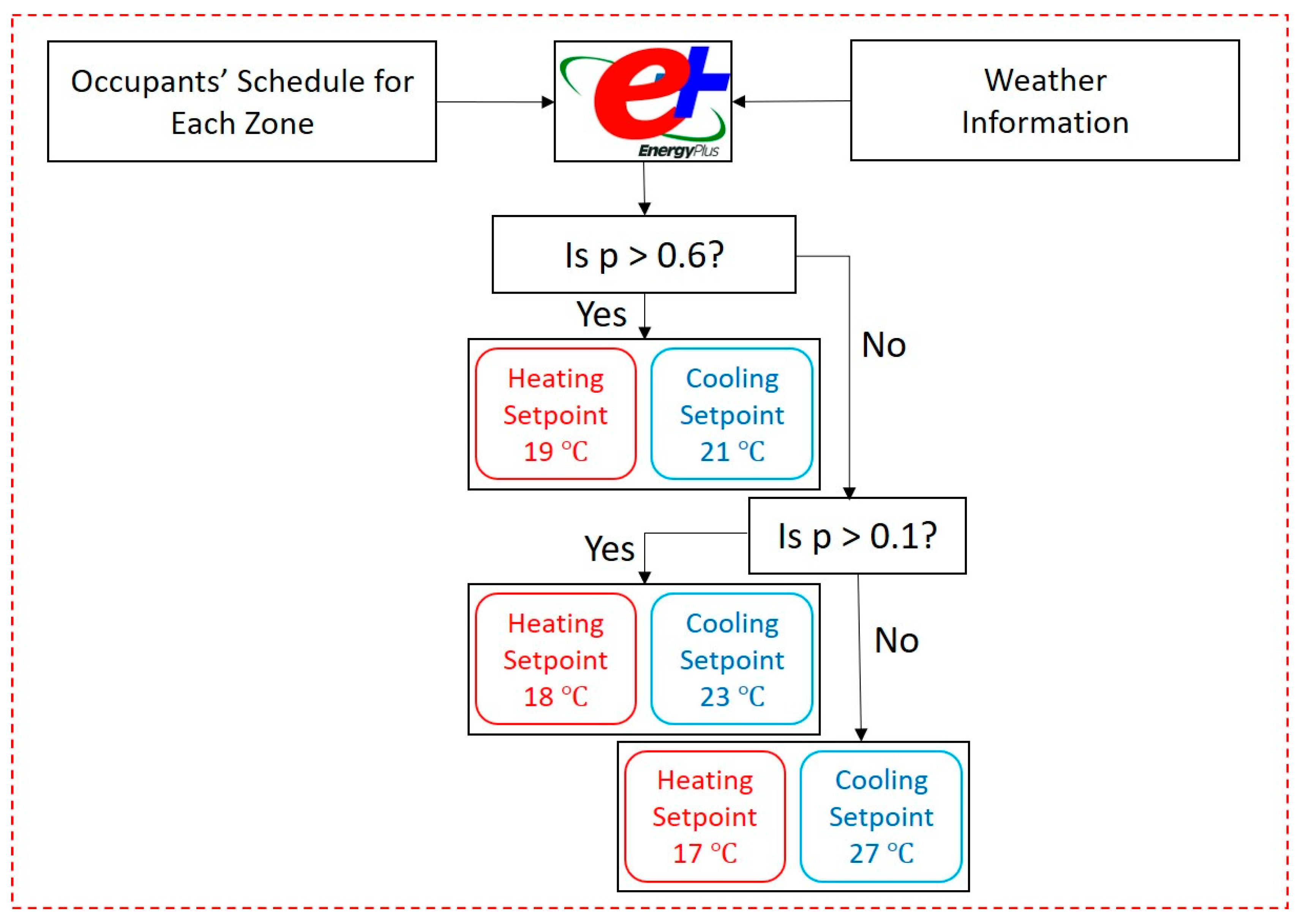
In this work, four different models are used for HVAC systems to see their impacts on energy and cost-saving. These models can be seen in Figure 1. The first model is the most basic thermostat in an office building. These thermostats continuously operate to maintain the space temperature at a fixed setpoint for heating and cooling purposes. The second model shows a thermostat schedule that is being used in most commercial buildings in arid climates. The heating and cooling setpoints and their schedules are constant, unless they are manually changed. Based on the working hour in a typical office building, the thermostats maintain the human comfort temperature between 7 a.m. to 4 p.m. In other times of the day, the setpoints are different than the working hours to reduce energy consumption while having a reasonable deviation from the comfort temperature range to decrease the ramping temperature. It is evident that this schedule is not optimal for all of the buildings in arid climates, since building characteristics and occupancy schedules are dissimilar. The third model is an occupancy-based model that uses the occupancy profile to assign the appropriate heating and cooling setpoints to the building zones. The occupancy schedule is given ahead of time by the building manager or can be forecasted by statistical methods or artificial intelligence models for each zone. This algorithm uses the occupancy percentage as a measure for describing a zone as occupied or vacant. If this value is greater than 60%, then the setpoint temperatures are 19 °C and 21 °C for heating and cooling, respectively. If it is less than 10%, the zone is assumed to be vacant and the HVAC systems can be turned off. Because some thermostats do not allow turning off, the heating and cooling setpoints are 17 °C and 27 °C in this case. If the percentage of the occupants’ presence is between 10% to 60%, the zone is semi-occupied and the heating and cooling setpoint temperatures are 19 °C and 23 °C, respectively. The deadband between heating and cooling setpoints has been taken into account to choose the proper setpoints for the first three algorithms. The deadband is a temperature range in which neither the heating nor the cooling system turns on, and it also does not let the thermostat activate heating and cooling in rapid succession. If this range is too narrow, both heating and cooling systems may be running simultaneously. Accordingly, at least a 2 °C difference between heating and cooling setpoints are considered in the proposed models to respect the deadband. The last model is an occupancy-based optimization algorithm that considers the building characteristics, weather conditions, electricity price, and the occupancy profile to minimize total electricity cost and output the optimal cooling setpoint. The proposed model uses the Monte-Carlo simulation method to find the probabilistic occupancy presence profile. Additionally, it is able to capture thermodynamic relationships for building zones. These algorithms tested on a simulated office building to see the effect of optimal cooling control on energy and cost-saving while aiming to simultaneously maintain human comfort. The first three control models can be used for both heating and cooling systems; however, the last one is only designed for cooling systems.

3. HVAC Control Models

In this section, the proposed HVAC control models are presented. The first model is a simple always-on model used in office buildings with traditional cooling systems, as discussed before. The second model is a control algorithm implemented in most office buildings located in countries with hot weather, such as Qatar. This model is a schedule-based algorithm that depends on the day’s time to assign setpoints, as shown in Figure 1. During working hours, the cooling and heating setpoints are 21 °C and 19 °C, respectively; otherwise, they are 27 °C and 17 °C. These two models are simple control algorithms that are used for the sake of comparison with the other two models. The third model is an occupancy-based model that takes the occupancy schedule of a zone into account in order to assign the appropriate setpoint temperature. The last model is a non-linear programming model, which is a modified version of the work Pinzon et al. [12] conducted. They presented a mixed-integer non-linear programming model to optimize the buildings’ operation in a microgrid using the management of cooling systems. In this work, an optimization model is proposed based on the revised version of their algorithm while using the occupancy schedule as one of this model’s inputs that affects the constraints and changes the optimal setpoint temperatures for each zone. In the following, detailed explanations and formulations of the third and fourth models are discussed.

3.1. Occupancy-Based Model

Occupancy data are difficult to acquire and precise ground truth values are rare, as most buildings do not have sufficient infrastructure to sense people accurately throughout the building [35]. The proposed occupancy-based model operates according to the current occupancy information. It uses the occupancy presence profile for describing the vacancy of a zone to come up with an appropriate setpoint for HVAC systems based on the following flowchart:
Figure 2 illustrates that each zone’s occupancy profile feeds the EnergyPlus model of the office building. The model then makes decisions to assign setpoint temperatures to each zone that are based on the occupants’ presence percentage.

3.2. Non-Linear Programming Model

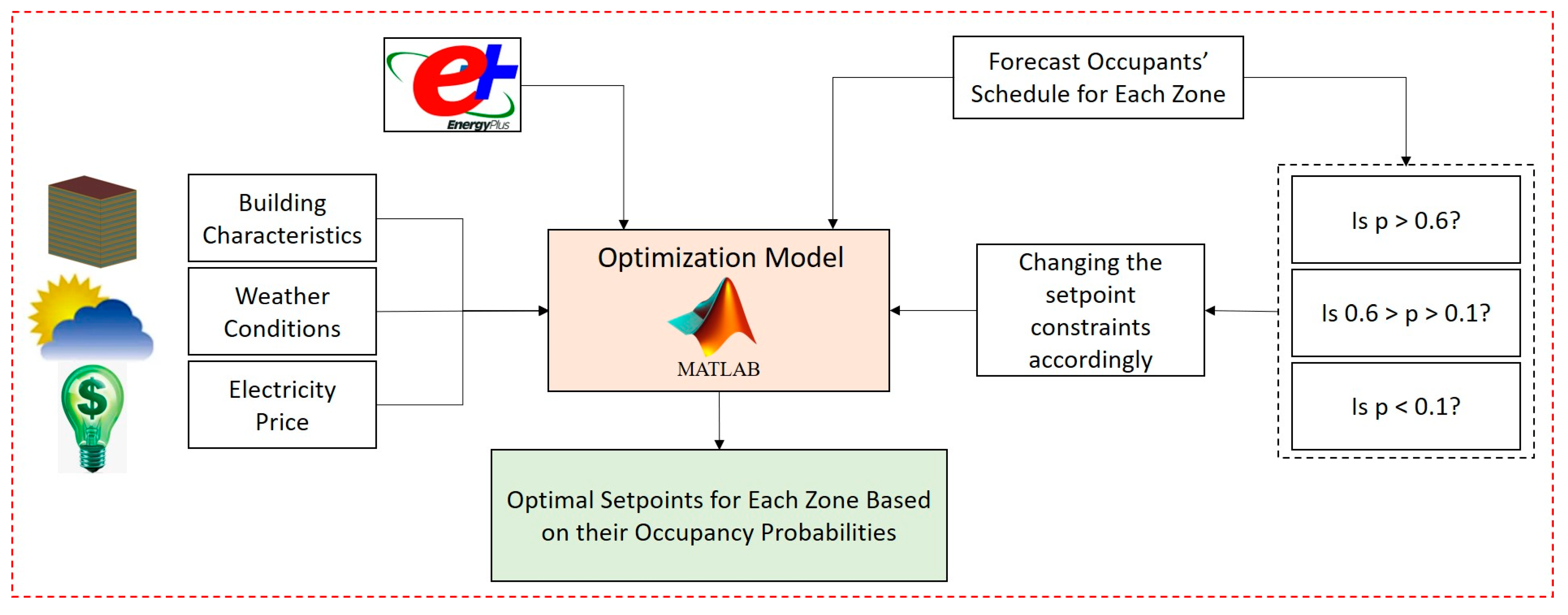
The optimal setpoints are usually different than the setpoints that come from the rule-based algorithms. This may cause a considerable waste of energy and money. A more reliable and accurate model is required to calculate each zone’s optimal setpoint that is based on the probabilistic occupancy schedule while maintaining human comfort. In this section, an NLP model is proposed to deal with the thermodynamic equations of a single building’s cooling system. The proposed model includes a cooling system for each zone comprised of a single-speed cooling coil and a constant volume fan. This model is able to assign the optimal day-ahead and near real-time cooling setpoints for each thermal zone of the building based on the occupancy schedule profile. In this model, the Monte-Carlo simulation method is used to determine the occupants’ presence profile. The optimization makes the control system decide at what time of the day to switch to lower or higher setpoint temperatures. The occupancy schedule profile is used twice in the mathematical formulations; first, in one of the constraints (Equation (15)) to calculate the sensible heat gain from the occupants; and, second, it is used to define the thresholds for the minimum and maximum allowable setpoint temperatures according to the presence of the people. Building characteristics, electricity costs, and weather data are the other inputs of this model. Figure 3 shows the flowchart of the NLP model. In the following, the Monte-Carlo method that is used to find the occupancy schedule is introduced first, and the optimization algorithm is then explained.

3.2.1. The Monte-Carlo Simulation Method for Determining the Occupancy Schedule

There are already several works in the literature considering probabilistic models for the occupancy presence profile in buildings. The work that Page et al. presented is one of the most prominent models in this field [36]. They proposed a generalized stochastic model for the occupancy simulation while using the presence probability and a parameter of mobility. This parameter is defined as the ratio between the probability of change of the state of presence over that of no change. In this article, we use the Page model to determine the commercial building’s occupancy presence profile. This profile will then be fed into the optimization model to obtain the optimal cooling setpoints. They developed their models based on the hypothesis that the probability of an occupant’s presence at the next time-step only depends on their presence at the current time-step. Accordingly, there is a general case of an inhomogeneous Markov chain with discrete states and discrete time-steps. The probability that an occupant is present at time-step t + 1 equals to:
P ( t + 1 ) = P ( t ) T 11 ( t ) + ( 1 P ( t ) ) T 01 ( t ) .
P ( t + 1 ) and P ( t ) are the probabilities of being present at time-steps t + 1 and t, respectively, as stated before. Page et al. defined the parameter of mobility to help them determine the values of T 01 ( t ) and T 11 ( t ) for all time-steps:
μ ( t ) = T 01 ( t ) + T 10 ( t ) T 00 ( t ) + T 11 ( t ) .
In this equation, T i j ( t ) is the transition probability from state i to state j at the time step t. Additionally, index 0 belongs to the absence state and index 1 introduces the presence state. For example, T 01 ( t ) is the transition probability from absence to the presence state at the time step t. They assumed that μ ( t ) is constant to simplify the inputs to the model. By considering this assumption and Equations (1) and (2), the transition probabilities can be determined by:
T 01 ( t ) = μ 1 μ + 1 P ( t ) + P ( t + 1 ) ,
T 01 ( t ) = P ( t ) 1 P ( t ) ( μ 1 μ + 1 P ( t ) + P ( t + 1 ) ) + P ( t + 1 ) P ( t ) .
Additionally, we know that the other transition probabilities can be obtained by:
T 00 ( t ) + T 01 ( t ) = 1 ,
T 10 ( t ) + T 11 ( t ) = 1 .
The inputs of the Page model are the presence probability profile and the parameter of mobility. One-hundred run periods of the Page model are simulated using the Monte-Carlo simulation method to develop an occupancy presence profile in this work. These simulations were implemented in MATLAB (R2018a, MathWorks, Torrance, CA, USA). After performing these runs, the occupants’ presence profiles are obtained by averaging the simulated runs’ hourly occupied ratio.

3.2.2. The Optimization Algorithm

Objective Function

The NLP model aims to minimize the total cooling energy cost, as follows:
M i n { t = 1 τ c t · P t } .
In Equation (7), c t is the real-time price of electricity and P t is total imported electricity from the main grid that equals to:
P t = P b t + ( i = 1 Z Q i t ) / Δ t .
Accordingly, the objective function can be revised, as follows:
M i n { t = 1 τ c t · ( P b t + ( i = 1 Z Q i t ) / Δ t ) } .

Constraints

P b t is the baseload of the building in time t and Q i t is the required cooling energy. This energy is consumed to cool down the building zones while considering the occupants’ presence percentage. The cooling system of a zone includes an electric chiller with a cooling fan. The required energy for cooling a zone is calculated by:
Q i t = ( C C i t φ i t μ i t + P fan i t ) Δ t .
In Equation (10), C C i t is the total cooling capacity, φ i t is energy input ratio, μ i t is the fraction of the time step during which the unit works at full capacity, and P fan i t is the fan power. In this equation, C C i t and φ i t are adjusted to the real operating conditions. These conditions are described in Equations (11) and (12) based on the performance curves that are explained in [36] while using cooling capacity modifier factors and energy input ratio factors.
C C i t = C C T i t R Q i ,
φ i t = E I T i t / C O P i .
In these equations, C C T i t and E I T i t are the factors to simulate the real operating conditions of the cooling system. Both of the factors are functions of outdoor dry-bulb temperature entering the cooling system and the average indoor wet-bulb temperature in the thermal zone. In Equation (10), the required cooling energy is calculated based on the total cooling capacity ( C C i t ) and energy input ratio ( φ i t ). The modifier factors C C T i t and E I T i t in Equations (11) and (12) are used to reflect the effect of weather conditions (e.g., outdoor temperature, and humidity) on the nominal cooling capacity ( R Q i ) and the coefficient of performance ( C O P i ). These factors are calculated based on the formulation that is presented in [35].
Besides, Equation (13) illustrates that the required cooling energy should be between the minimum and maximum cooling power capacity.
P m i n Δ t Q i t P m a x Δ t .
The cooling load of each zone, ambient weather, and building characteristics are the main elements that affect HVAC energy consumption. Equation (14) shows how to calculate the cooling load ( C L i t ) that is based on the sensible heat gains ( S H G i t ), the air volume thermal inertia ( Q S A i t ), the infiltration heat gain ( Q I i t ), and the heat through the surfaces ( Q S i t ).
C L i t = S H G i t Q S A i t + Q I i t + Q S i t .
The sensible heat gain is the heat that is generated by internal heat sources such as building occupants. Equation (15) describes this heat source, where α i t is the occupants’ schedule for each zone at each time-step, N P i is the peak occupancy for each zone, and h p ¯ is the average heat gain for each person.
S H G i t = α i t N P i h p ¯ .
The air volume thermal inertia and the infiltration heat gain are expressed by Equations (16) and (17).
Q S A i t = ρ a i r c p a i r V i ( T i t T i t 1 ) / Δ t ,
Q I i t = ρ a i r c p a i r V ˙ inf i ( T a m b t T i t ) .
The comfort index is defined by Equation (18) in order to address the human comfort conditions inside the zones. In this equation, C T i is the comfortable temperature setpoints and Δ T i t is the difference between the actual setpoint and comfortable setpoint [37].
C F T i t = 1 ( Δ T i t / C T i ) 2 ,
Δ T i t = T i t C T i .
The average comfort index during the total occupied period of each zone ω   α i t should be greater than a threshold, as shown in Equation (20). Additionally, based on what was recommended in [37], Equation (21) ensures that T i t is within the minimum and maximum comfortable temperature setpoints.
C F T i t C F T m i n ,
C T m i n i T i t C T m a x i ,
Based on the occupancy schedule for each zone, C T m i n i and C T m a x i will vary for different percentages of occupants’ presence. Table 1 describes these values for cooling.
The objective function (Equation (9)) should be solved when considering the constraints 10–21 in order to find the optimal setpoints for each zone. However, solving such a non-linear problem is very complicated and non-linearities should be removed by approximation.

Linearization Methods

In this article, the proposed method in [9] is used to linearize the non-linear equations. The non-linear constraints of this problem include Equations (11), (12), (14), and (18). The first two equations are non-linear due to the modifier factors that are quadratic functions. These factors depend on the operating conditions of the HVAC unit. These values can usually be found based on cooling performance curves. Additionally, another non-linearity comes from Equation (14) because of the nature of the heat through the surfaces ( Q S i t ). This heat can be found if the initial values for the surface heat and the temperature setpoint are known. These values can be calculated by using EnergyPlus for the simulated building. Hence, Q S i t for the first iteration and the later iterations can be found by Equations (22) and (23), respectively.
Q S i t = Q S i + ( T i T i t ) δ Q S i ,
Q S i t + 1 = Q S i t + ( T i t T i t + 1 ) δ Q S i ,
where Q S i is the initial surface heat, T i is the initial temperature setpoint, and δ Q S i is the heat increment that is used for the calculation of heat surface. Moreover, the run time fraction of the HVAC system is approximated based on the linear relationship with the part-load ratio of the cooling system ( θ i t ), as in Equation (24) [36].
μ i t = 0.991 θ i t + 0.039 .
θ i t in Equation (24) can be described by Equations (25)–(27). In these equations, Q V i t is the ventilation heat gain, Q L i t is the thermal fan loss, S H R i t is the sensible heat ratio modifier that can be found from [38], N S H R i t is the nominal sensible heat ratio, and η fan is the efficiency of the fan.
θ i t = C L i t + Q V i t + Q L i t S H R i t   N S H R i t   C C i t
Q V i t = ρ a i r c p a i r V ˙ fan i ( T a m b t T i t )
Q L i t = ( 1 η fan ) P fan i t
Note that Equation (25) is a linear constraint, since C C i t becomes constant after approximation of C C T i t . Moreover, Equations (28)–(31) present a piecewise linearization of the quadratic term of ( Δ T i t ) 2 in Equation (18).
Δ T i t = n = 1 N δ T i , n t
0 δ T i , n t δ T ¯ i
γ i , n = ( 2 n 1 ) δ T ¯ i
δ T i = ( C T m a x i C T m i n i ) / N
Hence, Equation (18) is rewritten based on Equation (32).
C F T i t = 1 ( ( n = 1 N γ i , n   δ T i , n t ) / ( C T i ) 2 )

Solution Methodology

In the above, we approximated the original NLP model by a linear programming (LP) model. This model requires the building’s physical characteristics, weather information, and the occupancy schedule profile. The linearized optimization problem has (Equation (9)) for its objective and Equations (10)–(17) and (20)–(32) for its constraints. The LP model is solved while using the MOSEK solver (MOSEK ApS, Copenhagen, Denmark) in MATLAB [39].

4. Simulated Building

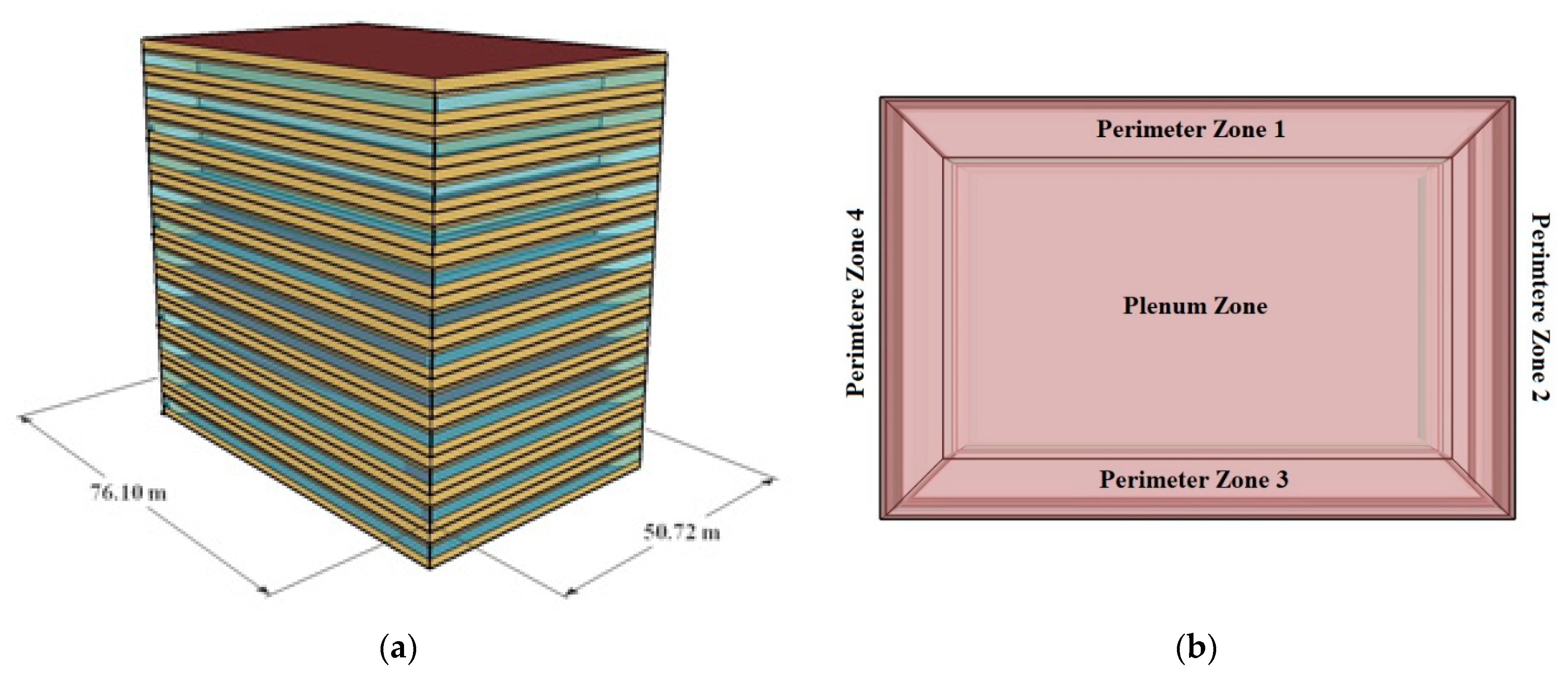
This article’s case study is constructed based on a large office building that is validated by US-DOE. The first three HVAC control algorithms are based on EnergyPlus building simulation models [36]. These rule-based methods feed the pre-defined criteria into the simulation. On the other hand, the fourth model employs the simulation results to generate the initial inputs and then uses this information in the proposed optimization approach. This 12-story building has 61 controlled thermal zones and a floor area of 46,320 m2. These zones include a basement, and five zones (as shown in Figure 4) for each floor. Each zone has a specific temperature profile, since its direction is different. For example, Perimeter Zone 1 is an east-facing zone that definitely has a different daily temperature profile than Perimeter Zone 3, which is a west-facing zone.
Figure 4 presents the original and X-ray geometry of this building. The aspect ratio, which is the overall length in the east-west direction divided by the overall length in the north-south direction, of this building is 1.5 [40]. Moreover, the building envelope was modified according to typical building characteristics that are located in countries with hot and humid weather conditions.

5. Results and Discussion

The proposed models for cooling control are applied to several case studies and the results are presented here. This section draws two general comparisons. First, the results for implementing different models to the simulated office building (Figure 4) in Doha are comprehensively shown and discussed. All of the control models are then implemented in the same building in four more cities: Phoenix, Miami, Barcelona, and Melbourne. The effectiveness of the proposed models on various case studies is then discussed and compared.

5.1. The Case Study of Doha

An office building in Doha is investigated in this section. The weather in Doha is blazing hot, with humid summer temperatures and mild winters. The city lies in the subtropical zone with a desert climate. Table 2 illustrates the weather data of Doha. These characteristics make its building need to operate their cooling systems almost all year, and smart control algorithms should be implemented to reduce the significant amount of energy that is used for cooling.

5.1.1. Cooling Control Models and Building Indoor Temperature

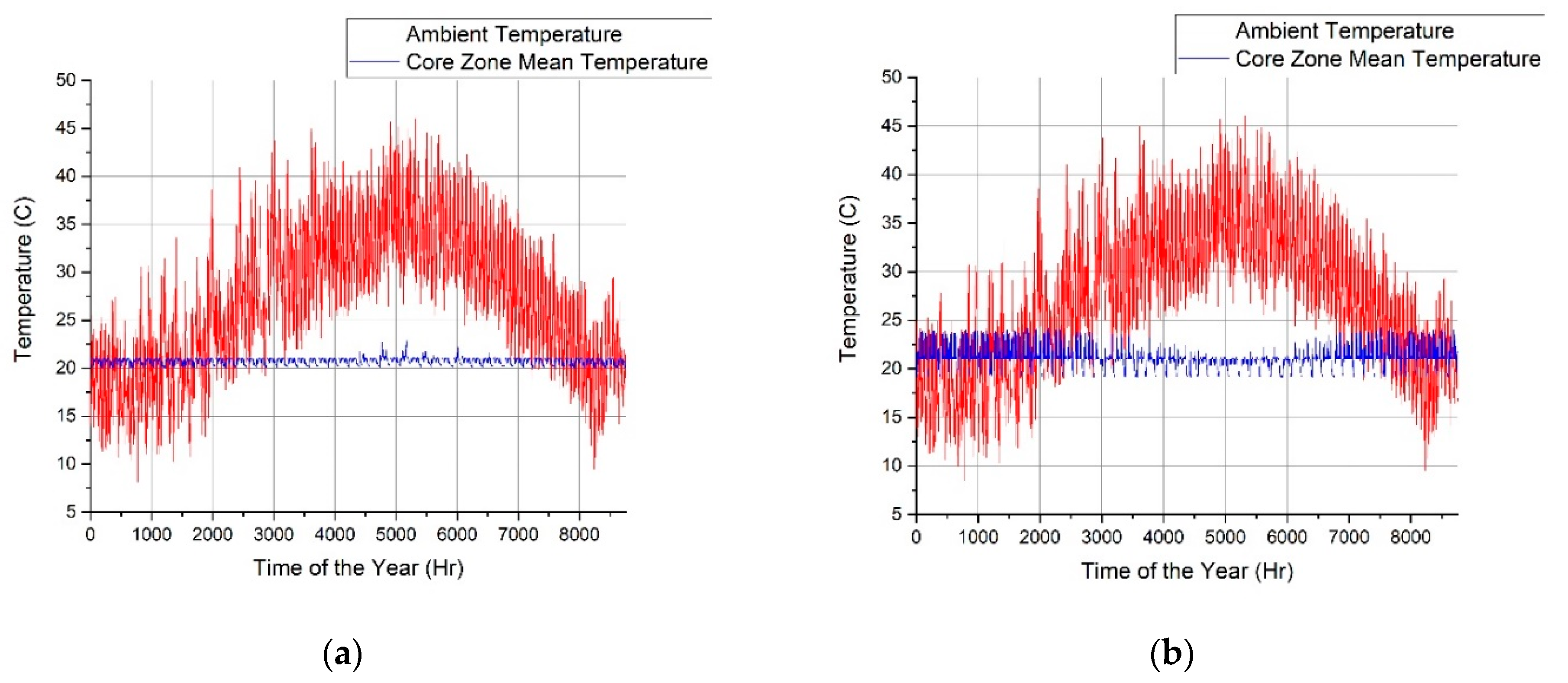
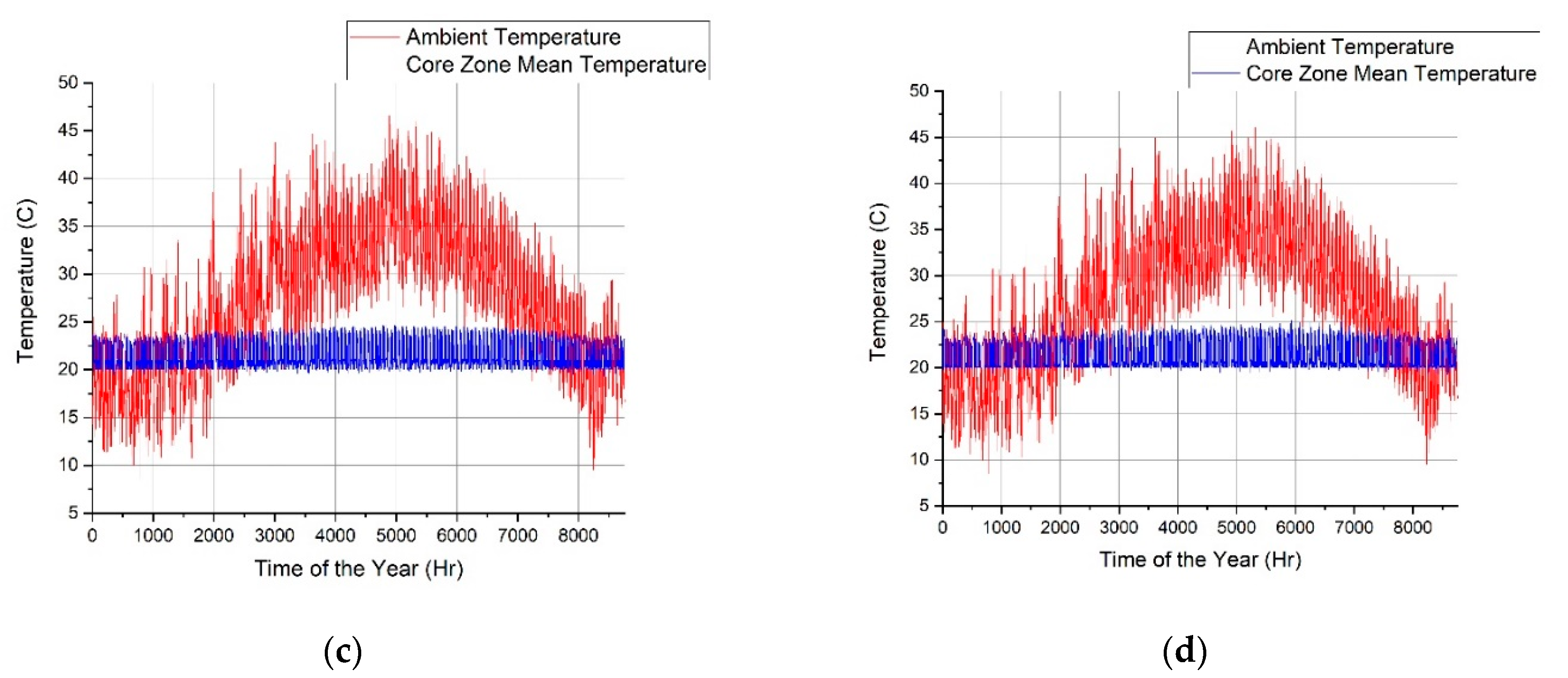
The control models mentioned above were applied to the case study that was described previously. This office building is located in Doha, Qatar, and the simulations are done in EnergyPlus. Figure 5 shows the ambient temperature and the indoor temperature of one of the building’s plenum zones during a year under the four control schemes. In this study, the base case is the schedule-based model, because it is currently being used in Doha’s office buildings. The results of other models will be compared to this model to describe their effectiveness in terms of cooling energy reduction and the total electricity and cost savings.
Figure 5a describes that the temperature of the zone is always around the cooling setpoint, and the deviation from the desired temperature is very low. Figure 5b illustrates a steadier indoor temperature during the cooling months. since the cooling systems are operating almost all the time. On the other hand, Figure 5c,d show that indoor temperature variation is noticeable when cooling control methods that are based on occupancy presence are used.
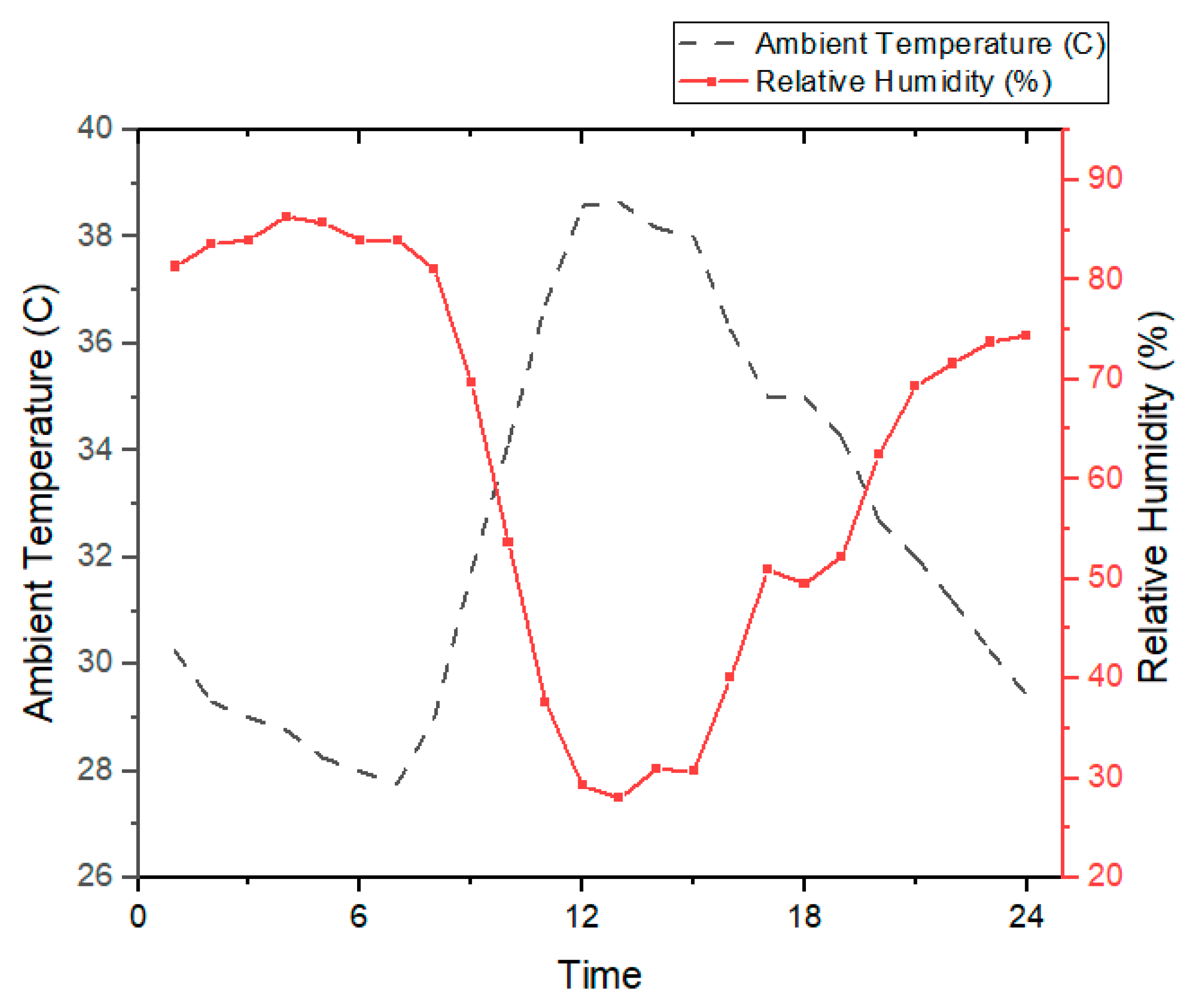
The results of the four cooling control models are also investigated for a typical summer day. Figure 6 shows the weather information for this representative day.
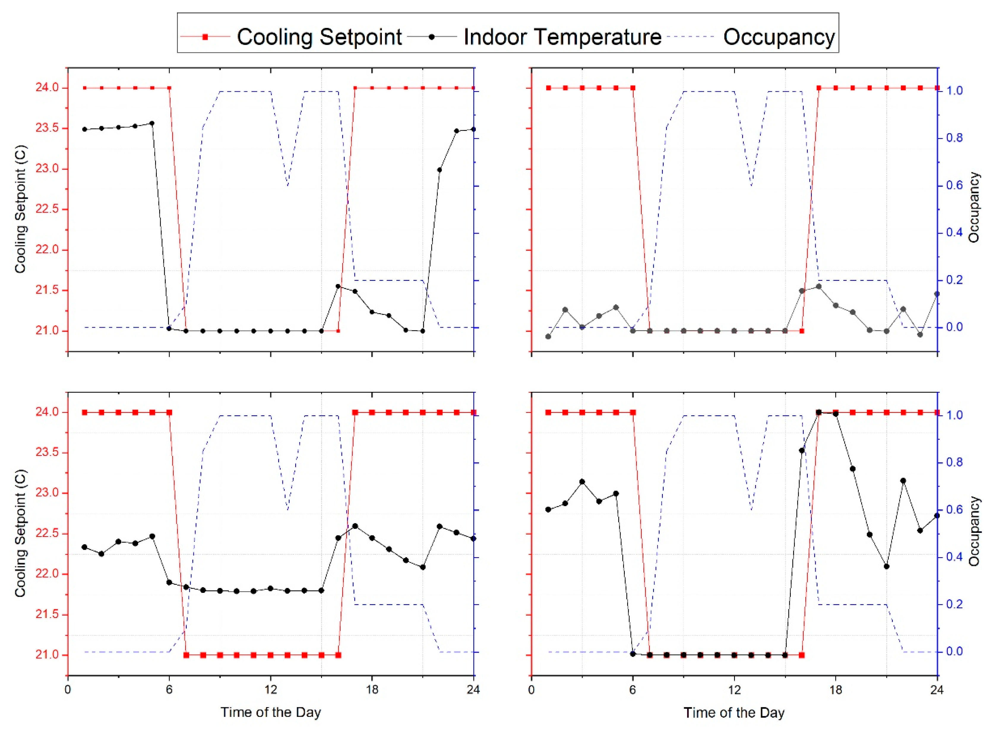
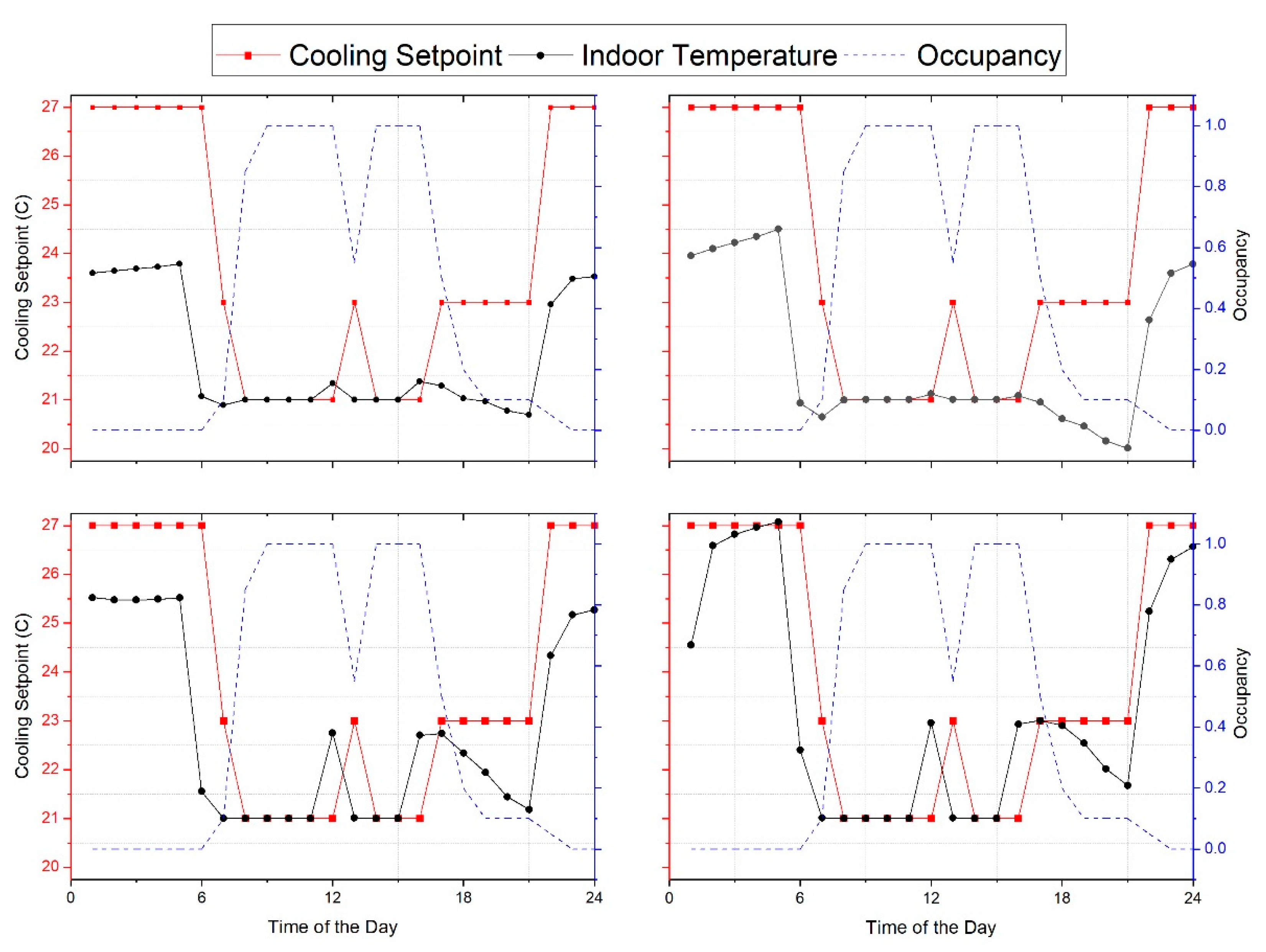
Figure 6 emphasizes the low humidity and high temperature of summers in Qatar. Accordingly, the need to use reliable and efficient cooling systems is inevitable. Each of the above four control algorithms has a specific effect on the building zones temperature, depending on the occupancy schedule and the zone location. Figure 7 and Figure 8 illustrate the occupancy schedule, cooling setpoints, and indoor temperature for four representative zones for schedule-based and occupancy-driven methods, respectively. Each representative zone is facing a specific direction.
Each zone’s thermal response is not very sensible to the occupancy pattern, as shown in Figure 7. Most of the zones have a relatively low indoor temperature, even if there are no occupants in the zone. On the other hand, Figure 8 shows that, as the occupant arrives in the morning to the selected zones, the assigned setpoint drops and thermal comfort are satisfied. On the other hand, after the zones become vacant, the setpoint grows and the indoor temperature increases accordingly by lowering the air conditioning system operation. Note that the outdoor temperature and humidity have an undeniable effect on the indoor temperature. For example, in the late afternoons and evenings, although the cooling setpoint is increased, the indoor temperature goes down a little bit first because of the outside temperature drop, and then it adjusts for the cooling setpoint increase. In this method and the NLP model, the average temperature is usually the same as the assigned setpoint, because the setpoint temperature assignment is based on zone thermal behavior prediction.

5.1.2. The Impact of Near Real-Time Occupancy Schedule on Cooling Setpoint Temperatures

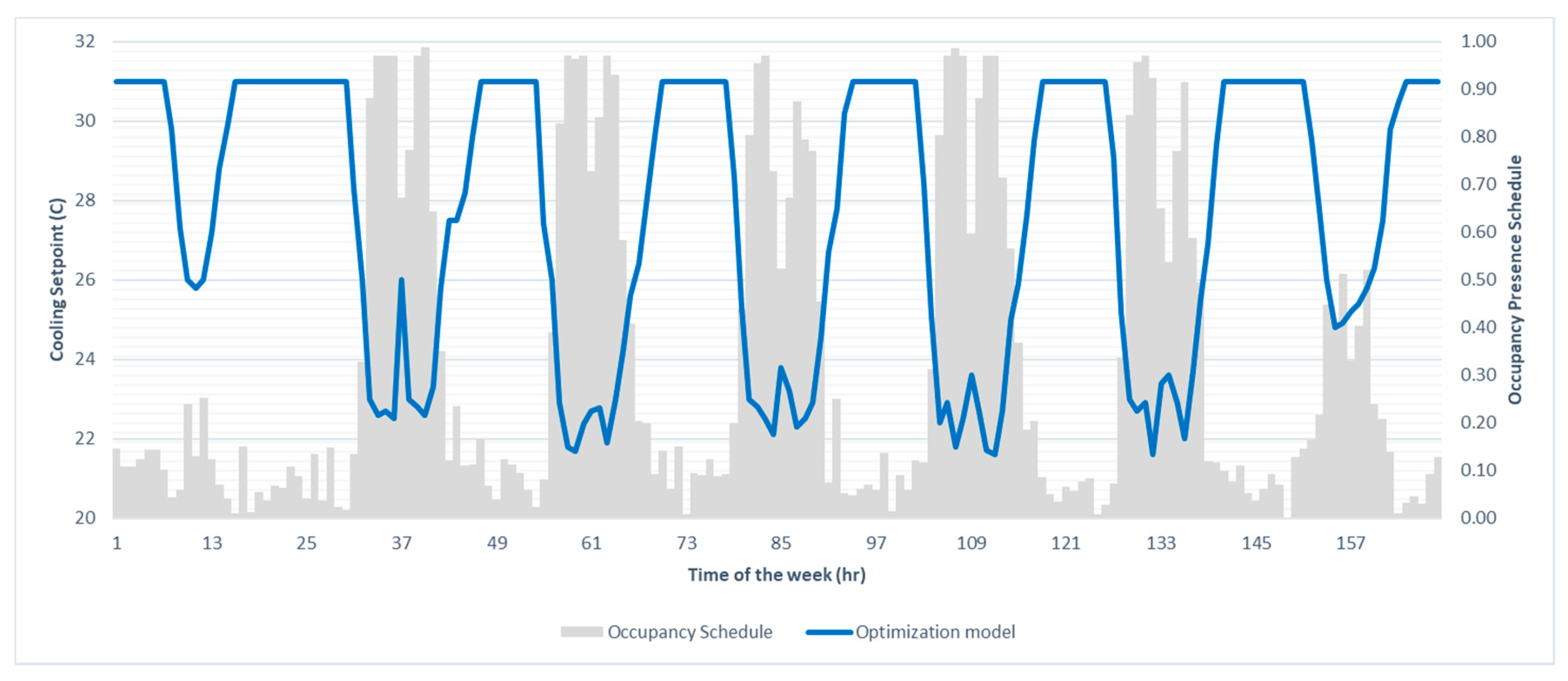
In this section, the proposed optimization model is used to determine the impact of the building’s near real-time schedule on the cooling setpoints. It is assumed that the occupancy schedule for the simulated building is updated each hour during the days. For example, the system receives the occupants’ presence schedule in each office from 10 a.m. to 11 a.m. at 9 a.m. Subsequently, this updated occupancy information feeds into the models for near-real-time cooling control. Figure 9 shows the schedule for a central zone of the office building for a representative summer week, along with the assigned cooling setpoints from the optimization model.
In this Figure, it can be seen that the optimization model is able to capture the occupancy schedule variation by assigning appropriate setpoint temperatures to maintain human comfort while minimizing the cooling energy consumption. Additionally, the setpoint slopes in the optimization model are reasonable. In this model, the following constraint (Equation (21)) helps to reduce the allowable range for the optimal setpoint based on the occupancy schedule, leading to a reduction in the setpoint temperature variation.
C T m i n i   T i t C T m a x i
This can remarkably affect the cooling energy consumption, since a sudden change of the setpoint results in more energy to overcome the zone’s thermal inertial to reduce or increase the average indoor temperature.

5.1.3. Cooling Energy Consumption in All Cooling Control Models

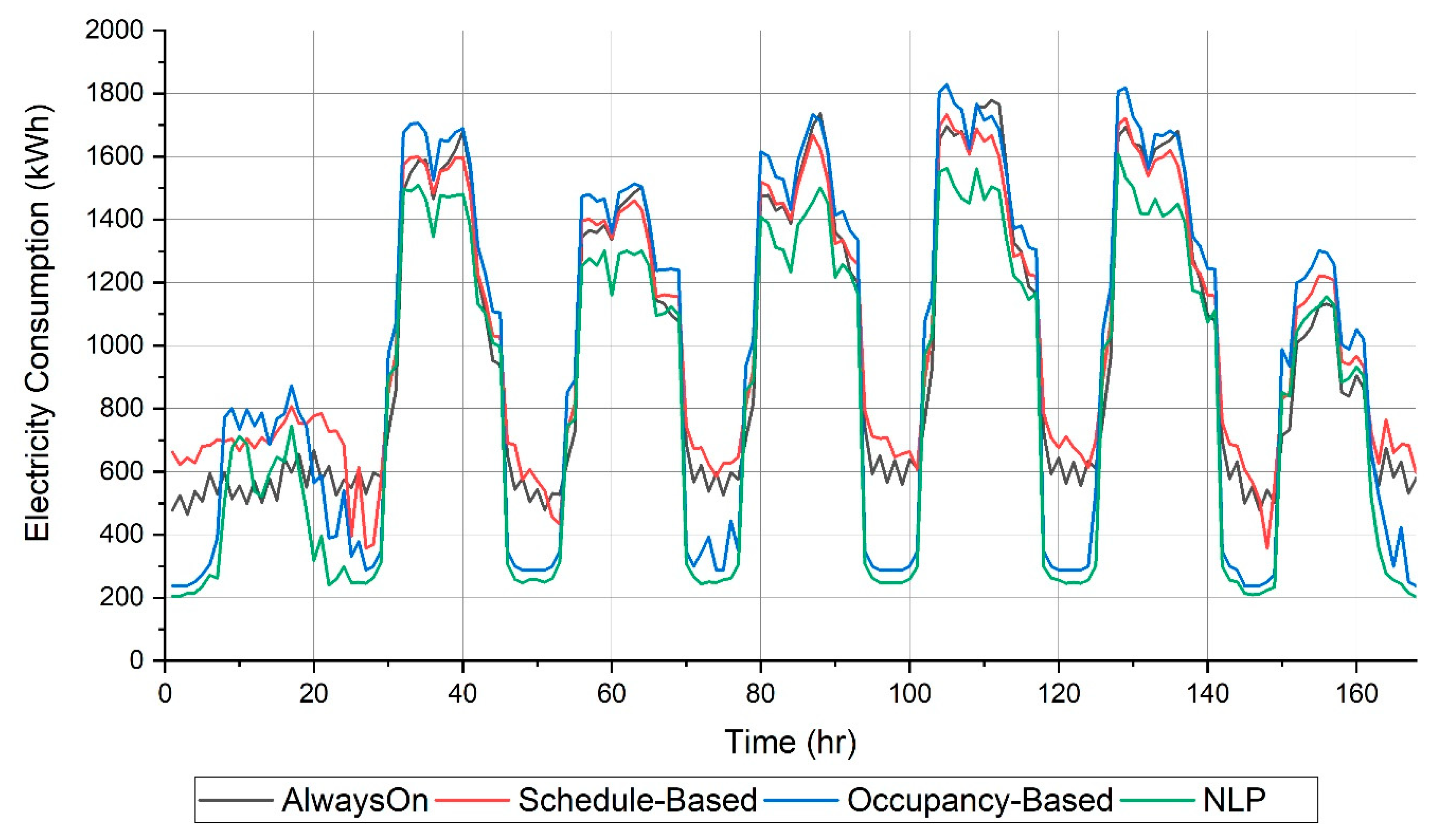
Figure 10 describes the effect of all four cooling control models on the total electricity consumption during a representative week in summer. This figure reveals that the non-linear optimization model has the lowest energy consumption during the time that zones are mostly unoccupied. Besides, it can be seen that energy consumption noticeably increases because of the occupant behavior that results in longer cooling operation time and lowering the cooling setpoint. Another interesting takeaway is that the always-on thermostat works more efficiently than the schedule-based control and it makes the building consume less energy. One of the main reasons for that is that it reduces the need for sudden increases and drops of indoor temperatures. These prompt variations require a great deal of energy to meet the human comfort level inside the buildings.

5.1.4. Comparison between All Control Strategies

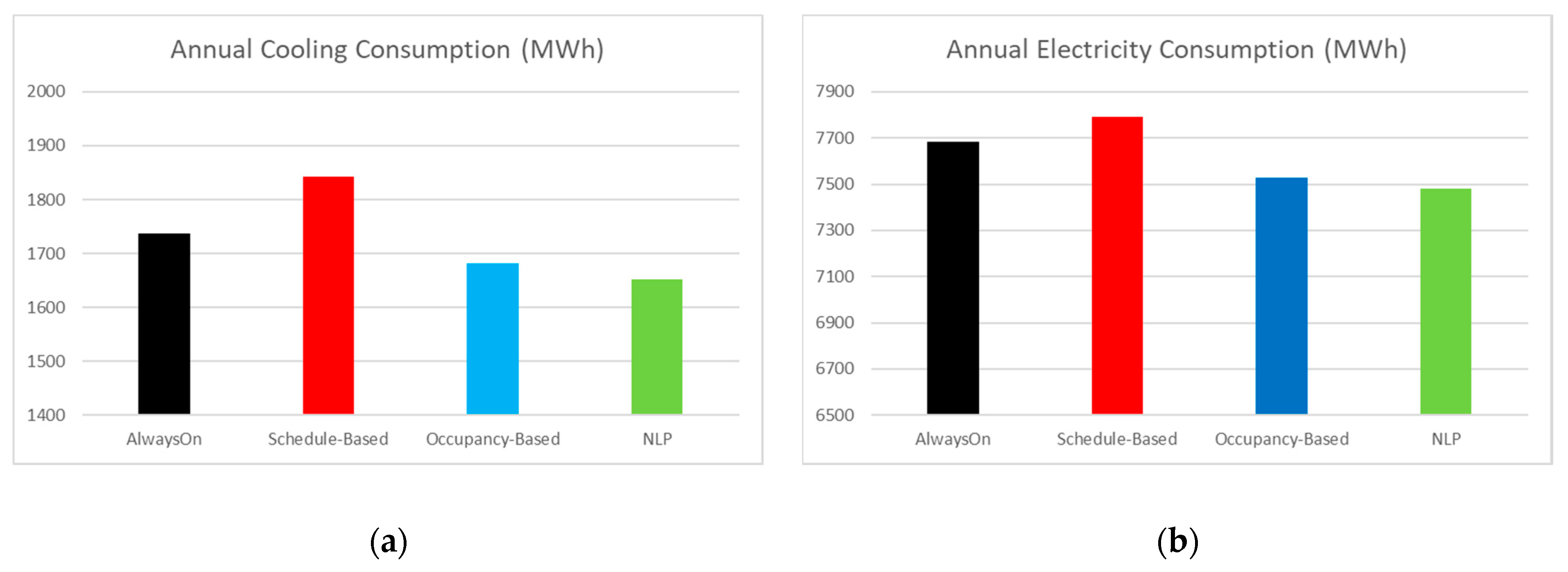
The energy consumption is significantly dependent on the cooling control methods, especially in Qatar, where the buildings need to run the cooling system almost 80% of the year. Figure 11 shows the comparison of annual electricity consumption and yearly cooling energy between the four control models. One of this study’s goals is to determine how the occupant schedule affects cooling energy and the total electricity consumption of an office building if zone setpoints are based on the occupant presence schedule. The optimization approach illustrates a noticeable advantage when compared to the current cooling control method (schedule-based technique) in Doha’s simulated office building. This figure describes that even a deterministic day-ahead occupancy-driven model can hugely reduce this building’s energy consumption.

5.2. The Implementation of the Control Models on the Building in Different Cities

This section analyzes the impacts of the proposed cooling control strategies on the same office building as Section 5.1, but it is located in different cities. This will help to evaluate the effect of different weather conditions and geographical locations on cooling energy consumption. These cities include Miami and Phoenix in the United States, Barcelona in Spain, and Melbourne in Australia. The results for these four cities as well as the results for Doha, which were shown in the last section, are compared and the impact of the applied methods is discussed.
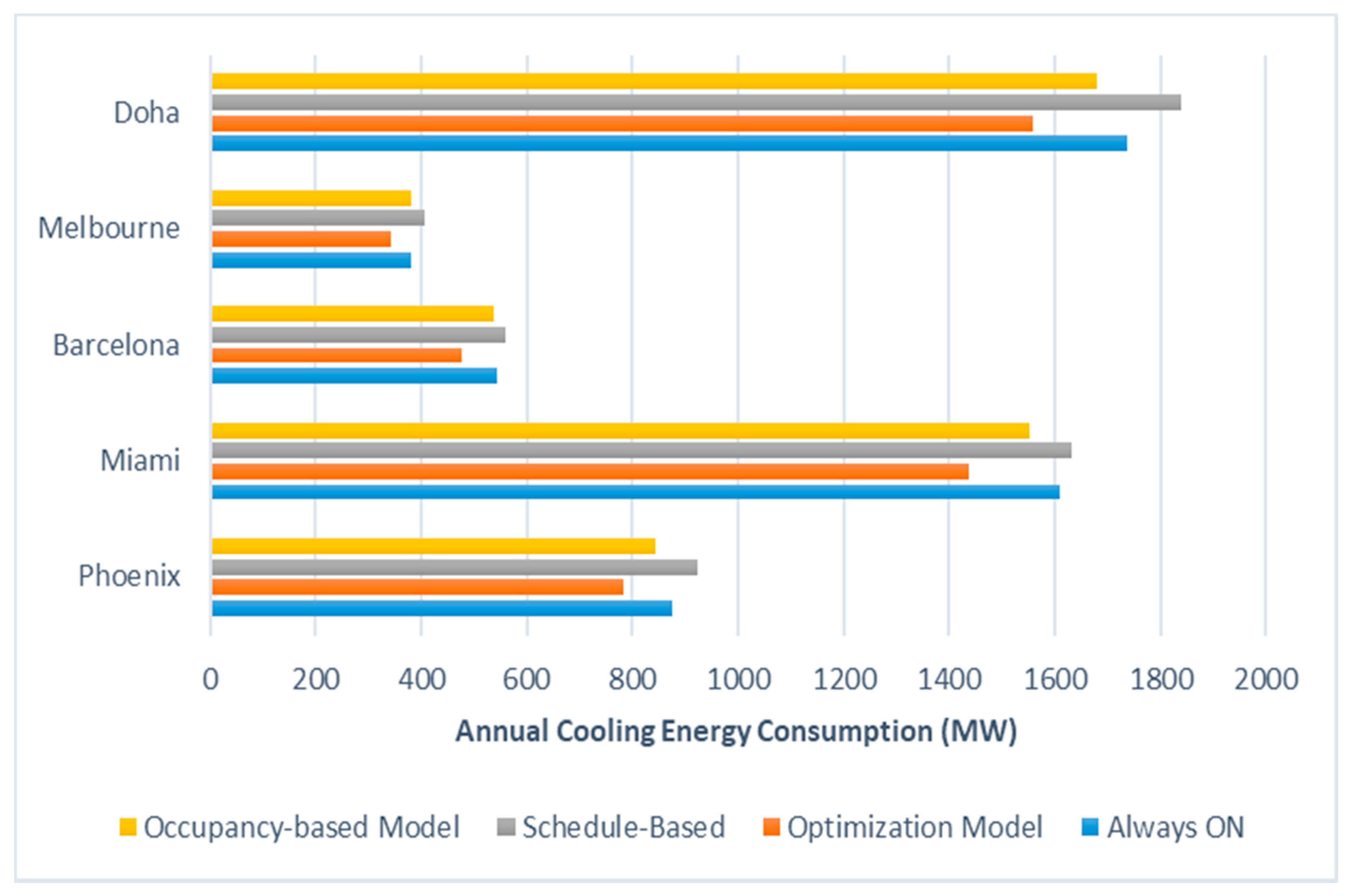
Figure 12 shows the cooling energy consumption after applying each model to the mentioned office building that is located in each city. It can be seen that the schedule-based model makes the building consume the highest amount of cooling energy in all case studies. This model does not consider thermal inertial in the building zones, and the cooling system is turned on or off only according to pre-defined schedules, which are not obviously optimal. Another interesting takeaway is that the optimization approach is able to minimize cooling energy consumption in all five case studies. The reduction amount is different for each case, due to the difference in weather conditions. For example, the NLP model’s impact on a building in Doha or Phoenix is noticeable due to the severe warm conditions in these cities and the need to implement more accurate cooling control methods. On the other hand, Melbourne and Barcelona have moderate weather characteristics on most days, which diminishes the possible saving effect of these models on the case studies in these cities.
The schedule-based model, which makes the building consume the highest amount of energy, is taken as a base case for all cities, in order to have a reasonable criterion for comparing the impact of the proposed models on the mentioned case studies. Subsequently, the percentage of saving in cooling energy consumption for all other models is compared with the base case for each case study, as illustrated in Table 3.
This table proves the effectiveness of the optimization model. This approach is capable of reducing the cooling energy consumption up to 15.19% in an office building in the city of Phoenix. Moreover, Table 3 demonstrates that the always-on thermostat would work better than the schedule-based in all cases. It happens due to the reduction of increases and drops of building indoor temperature that saves energy. Additionally, it can be seen that the proposed optimization model is able to save energy around 15% annually in an office building located in Doha and Phoenix, which is noticeable and it can play a significant role in the total energy consumption of building sectors if it will be applied to several office buildings in those locations.

5.3. Discussion

The simulated building in this paper is designed to be very similar to an actual office building in arid climates, so the proposed models can be applied to the existing commercial buildings. However, using a single office building may limit the generalizability of the results that are illustrated in this paper. Although occupants’ presence and human comfort are considered in this study, the dynamic nature of occupants’ behavior will make a remarkable variation in their needs to lower or increase the setpoint temperatures. Note that several works, including this article, assumed that each zone could have a separate setpoint temperature and follow a different HVAC control algorithm to help the building minimize its total energy consumption. In order to use these control systems, the buildings are required to be designed when considering these assumptions with a smart HVAC control system. Currently, connecting a central HVAC control system that can optimize the zone setpoints to the Building Automation System (BAS) is becoming more popular in new commercial buildings. This connection makes the facility more energy-efficient without the need to manually change the zone setpoints by the building engineers.
Occupant surveys are a good source of information for data collection in order to develop reliable control models. Another important fact is that the expectations of temperature and relative humidity in different climates notably impact people’s perceptions of their environment. For example, in subtropical regions, people may accept higher cooling setpoint temperatures when they compare the indoor temperature with the ambient temperature that could be very hot and humid and unbearable. Hence, it may result in higher cooling setpoint temperatures, which leads to energy and cost-saving.

6. Conclusions

In this paper, a non-linear optimization approach was proposed for smart cooling control of the buildings in order to minimize the total energy costs while maintaining the occupants’ comfort level. The proposed optimization model used the Monte-Carlo simulation method to determine the probabilistic occupancy schedule. It also considers the weather information, building characteristics, and the electricity pricing profile to calculate the optimal cooling setpoint temperatures for all building zones. This model was then compared with three other cooling control models, including the always-on thermostat, the schedule-based model, and the rule-based occupancy-driven model. These methods were implemented in a simulated office building, and the results showed considerable energy saving through cooling energy systems.
In this work, the Monte-Carlo method was used to predict the occupancy schedule. Future studies can focus on applying different stochastic models to the proposed optimization approach to provide more accurate insight into the random variation in people’s presence in building zones over time. Additionally, the results presented here are drawn based on the simulation of an office building. However, the investigation of the impact of different cooling control systems on real buildings will be helpful, since building energy simulation can suffer from various errors, such as weather data deviation and the simplification used in the building simulation software.

Author Contributions

The following contributions were made to this research: Conceptualization and Original Idea, E.Z. and M.A.J.; Methodology and Investigation, S.D.N. and M.A.J. and E.Z.; Model Development, Optimization, Simulation and Visualization, S.D.N.; Supervision, M.A.J.; Writing Original Draft, S.D.N.; Writing Review and Editing, M.A.J. and E.Z.; Funding Acquisition, E.Z.; All authors have read and agreed to the published version of the manuscript.

Funding

This publication was made possible by an NPRP award [NPRP11S-1228-170142] from the Qatar National Research Fund (a member of the Qatar Foundation). The statements made herein are solely the responsibility of the authors. The publication of this article was funded by the Qatar National Library.

Conflicts of Interest

The authors declare no conflict of interest.

Nomenclature

Parameters
c t Electricity cost at time t
P m i n The minimum power of the cooling system (W)
P m a x The maximum power of the cooling system (W)
Δ t Time-step duration
R Q i Rated total cooling capacity for the cooling system of zone i (W)
C O P i Coefficient of performance for the cooling system of zone i
V ˙ fan The volume flow rate of the fan (m3/s)
S H G i t The sensible heat gains from people inside zone i (W)
N P i The maximum number of people in zone i
h p ¯ The average heat gain for each person (W)
V i The volume of zone i (m3)
V ˙ inf i The volume flow rate of infiltration (m3/s)
c p a i r The specific heat of air (J/gr. °C)
ρ a i r The density of air (kg/m3)
T a m b t The ambient temperature (°C)
C T i The comfortable temperature setpoint (°C)
C F T m i n The minimum comfort index
C T m i n i The minimum allowable temperature (°C)
C T m a x i The maximum allowable temperature (°C)
Q S i The initial surface heat gain (W)
T i The initial temperature setpoint (°C)
δ Q S i Heat increment to define Q S i (W)
η fan The efficiency of the fan
δ T i , n t Discretization steps of the piecewise linearization for Δ T i t
N Number of blocks for the piecewise formulation
γ i , n The slope of the nth block in piecewise linearization for Δ T i t
Decision variables
α i t Occupancy schedule at time t for zone i
P t Total cooling electricity consumption at time t (W)
P b t Base-load at time t (W)
Q i t Cooling energy for zone i at time t (J)
C C i t Total cooling capacity for zone i at time t (W)
φ i t Energy input ratio of cooling system for zone i at time t
μ i t Run time fraction of cooling system for zone i at time t
P fan i t Fan power for VAV system in zone i at time t (W)
C C T i t Cooling capacity modifier factor
E I T i t Energy input ratio modifier factor
C L i t The sensible cooling load (W)
Q S A i t The air volume thermal inertia (W)
Q I i t The infiltration heat gain (W)
Q S i t The surface heat (W)
C F T i t The comfort index
θ i t Part-load ratio of cooling system
Q V i t The ventilation heat gain (W)
Q L i t The thermal fan loss (W)
Indices
iIndex of zones
tIndex of time
nIndex of blocks used for the piecewise linearization
Sets
Ω T Set of time-steps
Ω Z Set of zones
Ω N Set of blocks for piecewise linearization

References

  1. International Energy Agency. Tracking Buildings. 2020. Available online: https://www.iea.org/reports/tracking-buildings-2020 (accessed on 20 June 2020).
  2. Pérez-Lombard, L.; Ortiz, J.; Pout, C. A review on buildings energy consumption information. Energy Build. 2008, 40, 394–398. [Google Scholar] [CrossRef]
  3. Harmon, A.; Truby, J.M. Achieving Green Building in Qatar through Legal and Fiscal Tools. J. Sustain. Dev. 2019, 12, 96–111. [Google Scholar] [CrossRef]
  4. Fahkroo, M.I.; Al-Awainati, N.; Musharavati, F.; Pokherel, S.; Gabbar, H.A. Operations optimization towards high performance cooling in commercial buildings. In Proceedings of the 2013 IEEE International Conference on Smart Energy Grid Engineering (SEGE), Oshawa, ON, Canada, 28–30 August 2013; pp. 1–6. [Google Scholar] [CrossRef]
  5. Ghofrani, A.; Nazemi, S.D.; Jafari, M.A. HVAC load synchronization in smart building communities. Sustain. Cities Soc. 2019, 51. [Google Scholar] [CrossRef]
  6. Ghahramani, A.; Zhang, K.; Dutta, K.; Yang, Z.; Becerik-Gerber, B. Energy savings from temperature setpoints and deadband: Quantifying the influence of building and system properties on savings. Appl. Energy 2016, 165, 930–942. [Google Scholar] [CrossRef] [Green Version]
  7. Lakeridou, M.; Ucci, M.; Marmot, A. Imposing limits on summer set-points in UK air-conditioned offices: A survey of facility managers. Energy Policy 2014, 75, 354–368. [Google Scholar] [CrossRef]
  8. Mui, K.; Wong, L.T.; Fong, N.K.; Wai, M.K. Optimization of indoor air temperature set-point for centralized air-conditioned spaces in subtropical climates. Autom. Constr. 2010, 19, 709–713. [Google Scholar] [CrossRef]
  9. Pinzon, J.A.; Vergara, P.P.; Da Silva, L.C.P.; Rider, M.J. An MILP model for optimal management of energy consumption and comfort in smart buildings. In Proceedings of the 2017 IEEE Power & Energy Society Innovative Smart Grid Technologies Conference (ISGT), Washington, DC, USA, 23–26 April 2017. [Google Scholar]
  10. Fan, B.; Jin, X.; Fang, X.; Du, Z. The method of evaluating operation performance of HVAC system based on exergy analysis. Energy Build. 2014, 77, 332–342. [Google Scholar] [CrossRef]
  11. Nazemi, S.D.; Mahani, K.; Ghofrani, A.; Amini, M.; Kose, B.E.; Jafari, M.A. Techno-Economic Analysis and Optimization of a Microgrid Considering Demand-Side Management. In Proceedings of the 2020 IEEE Texas Power and Energy Conference (TPEC), College Station, TX, USA, 6–7 February 2020. [Google Scholar]
  12. Pinzon, J.A.; Vergara, P.P.; Da Silva, L.C.P.; Rider, M.J. Optimal Management of Energy Consumption and Comfort for Smart Buildings Operating in a Microgrid. IEEE Trans. Smart Grid 2019, 10, 3236–3247. [Google Scholar] [CrossRef]
  13. Nazemi, S.D.; Jafari, M.A. An Automated Cluster-Based Approach for Asset Rescheduling in Building Communities. In Proceedings of the 2020 IEEE Texas Power and Energy Conference (TPEC), College Station, TX, USA, 6–7 February 2020. [Google Scholar] [CrossRef]
  14. Vaghefi, S.A.; Jafari, M.A.; Zhu, J.; Brouwer, J.; Lu, Y. A Hybrid Physics-Based and Data Driven Approach to Optimal Control of Building Cooling/Heating Systems. IEEE Trans. Autom. Sci. Eng. 2016, 13, 600–610. [Google Scholar] [CrossRef] [Green Version]
  15. Johnson, J.A.; Sastry, C.; Ning, X.; Patel, A.H. Srivastava, System and Method for Climate Control Set-Point Optimization Based on Individual Comfort. U.S. Patent 9,020,647, 28 April 2015. [Google Scholar]
  16. Ghofrani, A.; Nazemi, S.D.; Jafari, M.A. Prediction of building indoor temperature response in variable air volume systems. J. Build. Perform. Simul. 2019, 13, 34–47. [Google Scholar] [CrossRef]
  17. Kusiak, A.; Li, M.; Tang, F. Modeling and optimization of HVAC energy consumption. Appl. Energy 2010, 87, 3092–3102. [Google Scholar] [CrossRef]
  18. Afram, A.; Janabi-Sharifi, F.; Fung, A.S.; Raahemifar, K. Artificial neural network (ANN) based model predictive control (MPC) and optimization of HVAC systems: A state of the art review and case study of a residential HVAC system. Energy Build. 2017, 141, 96–113. [Google Scholar] [CrossRef]
  19. Kelman, A.; Borrelli, F. Bilinear Model Predictive Control of a HVAC System Using Sequential Quadratic Programming. IFAC 2011, 44, 9869–9874. [Google Scholar] [CrossRef] [Green Version]
  20. Ma, Y.; Borrelli, F. Fast stochastic predictive control for building temperature regulation. In Proceedings of the 2012 American Control Conference (ACC), Montreal, QC, Canada, 27–29 June 2012; pp. 3075–3080. [Google Scholar] [CrossRef]
  21. Rehrl, J.; Horn, M. Temperature control for HVAC systems based on exact linearization and model predictive control. In Proceedings of the 2011 IEEE International Conference on Control Applications, Denver, CO, USA, 28–30 September 2011; pp. 1119–1124. [Google Scholar] [CrossRef]
  22. Nassif, N. Modeling and optimization of HVAC systems using artificial neural network and genetic algorithm. Build. Simul. 2014, 7, 237–245. [Google Scholar] [CrossRef]
  23. Javed, A.; Larijani, H.; Ahmadinia, A.; Emmanuel, R.; Mannion, M.; Gibson, D. Design and Implementation of a Cloud Enabled Random Neural Network-Based Decentralized Smart Controller with Intelligent Sensor Nodes for HVAC. IEEE Internet Things J. 2017, 4, 393–403. [Google Scholar] [CrossRef] [Green Version]
  24. Kusiak, A.; Xu, G. Modeling and optimization of HVAC systems using a dynamic neural network. Energy 2012, 42, 241–250. [Google Scholar] [CrossRef]
  25. Ghofrani, A.; Jafari, M.A. Distributed air conditioning control in commercial buildings based on a physical-statistical approach. Energy Build. 2017, 148, 106–118. [Google Scholar] [CrossRef]
  26. Perez, K.X.; Baldea, M.; Edgar, T.F. Integrated HVAC management and optimal scheduling of smart appliances for community peak load reduction. Energy Build. 2016, 123, 34–40. [Google Scholar] [CrossRef] [Green Version]
  27. Javed, A.; Larijani, H.; Ahmadinia, A.; Gibson, D. Smart Random Neural Network Controller for HVAC Using Cloud Computing Technology. IEEE Trans. Ind. Inform. 2017, 13, 351–360. [Google Scholar] [CrossRef] [Green Version]
  28. Wang, C.; Pattawi, K.; Lee, H. Energy saving impact of occupancy-driven thermostat for residential buildings. Energy Build. 2020, 211, 109791. [Google Scholar] [CrossRef]
  29. Shi, J.; Yu, N.; Yao, W. Energy Efficient Building HVAC Control Algorithm with Real-time Occupancy Prediction. Energy Procedia 2017, 111, 267–276. [Google Scholar] [CrossRef]
  30. Aftab, M.; Chen, C.; Chau, C.-K.; Rahwan, T. Automatic HVAC control with real-time occupancy recognition and simulation-guided model predictive control in low-cost embedded system. Energy Build. 2017, 154, 141–156. [Google Scholar] [CrossRef] [Green Version]
  31. Agarwal, Y.; Balaji, B.; Gupta, R.; Lyles, J.; Wei, M.; Weng, T. Occupancy-driven energy management for smart building automation. In Proceedings of the BuildSys’10—2nd ACM Workshop on Embedded Sensing Systems for Energy-Efficiency in Building, Zürich, Switzerland, 3–5 November 2010. [Google Scholar]
  32. Kleiminger, W. Occupancy Sensing and Prediction for Automated Energy Savings. Ph.D. Thesis, ETH Zurich, Zürich, Switzerland, 2015. [Google Scholar]
  33. Wang, W.; Chen, J.; Hong, T. Occupancy prediction through machine learning and data fusion of environmental sensing and Wi-Fi sensing in buildings. Autom. Constr. 2018, 94, 233–243. [Google Scholar] [CrossRef] [Green Version]
  34. Candanedo, L.M.; Feldheim, V. Accurate occupancy detection of an office room from light, temperature, humidity and CO2 measurements using statistical learning models. Energy Build. 2016, 112, 28–39. [Google Scholar] [CrossRef]
  35. U.S. Department of Energy. EnergyPlus Engineering Reference; U.S. Department of Energy: Washington, DC, USA, 2015.
  36. Page, J.; Robinson, D.; Morel, N.; Scartezzini, J.-L. A generalised stochastic model for the simulation of occupant presence. Energy Build. 2008, 40, 83–98. [Google Scholar] [CrossRef]
  37. Wang, N.; Fang, F.; Feng, M. Multi-objective optimal analysis of comfort and energy management for intelligent buildings. In Proceedings of the 26th Chinese Control and Decision Conference (2014 CCDC), Changsha, China, 31 May–2 June 2014; pp. 2783–2788. [Google Scholar]
  38. Kruis, N. Reconciling differences between residential DX Cooling Models in DOE-2 and EnergyPlus. In Proceedings of the 4th National Conference IBPSA-USA, Boulder, CO, USA, 4–6 August 2010. [Google Scholar]
  39. MOSEK Optimization Toolbox for MATLAB. 2020. Available online: https://docs.mosek.com/9.2/toolbox.pdf (accessed on 14 March 2020).
  40. Deru, M.; Field, K.; Studer, D.; Benne, K.; Griffith, B.; Torcellini, P.; Liu, B.; Halverson, M.; Winiarski, D.; Rosenberg, M.; et al. U.S. Department of Energy Commercial Reference Building Models of the National Building Stock; U.S. Department of Energy: Washington, DC, USA, 2011.
  41. Climate Data, Doha Weather. 2019. Available online: https://en.climate-data.org/asia/qatar/doha/doha-6368/#climate-graph (accessed on 14 March 2020).
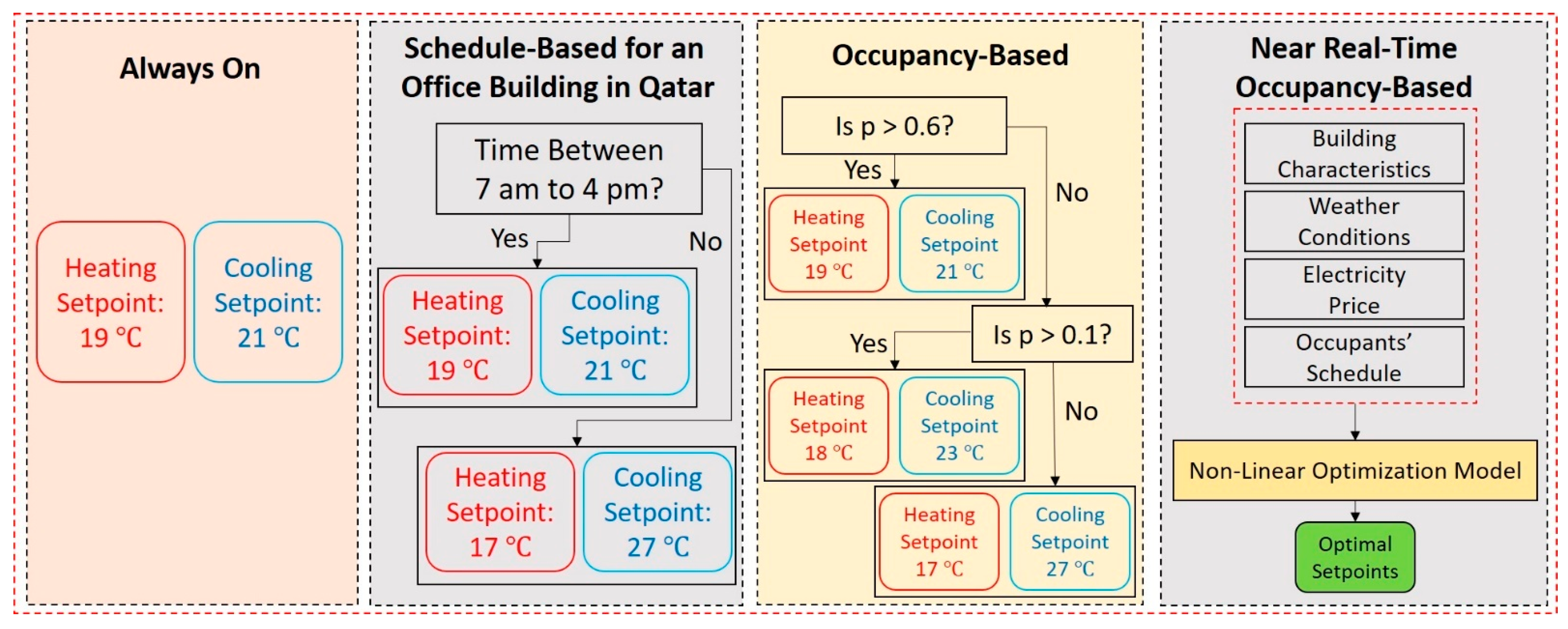
Figure 1. The flowchart of four different Heating, Ventilation, and Air Conditioning (HVAC) control system used in this work.
Energies 14 01722 g001
Figure 2. Explanation of the occupancy-based model.
Energies 14 01722 g002
Figure 3. The flowchart of the optimization model based on the occupancy schedule profile.
Energies 14 01722 g003
Figure 4. Simulated office building: (a) Original view; (b) X-ray geometry.
Energies 14 01722 g004
Figure 5. Ambient temperature versus the temperature of one of the plenum zones in the building by using the following models: (a) the always-on thermostat; (b) the schedule-based model; (c) the occupancy-driven model; (d) the optimization model.
Energies 14 01722 g005aEnergies 14 01722 g005b
Figure 6. A representative day for Summer in Qatar: ambient temperature and air relative humidity.
Energies 14 01722 g006
Figure 7. Occupancy schedule, indoor temperature, and optimal setpoint assignment for four selected zones according to the schedule-based model: (top-left) an east-facing zone; (top-right) a west-facing zone; (bottom-left) a south-facing zone; and (bottom-right) a north-facing zone.
Energies 14 01722 g007
Figure 8. Occupancy schedule, indoor temperature, and optimal setpoint assignment for four selected zones based on the occupancy-driven model: (top-left) an east-facing zone; (top-right) a west-facing zone; (bottom-left) a south-facing zone; and (bottom-right) a north-facing zone.
Energies 14 01722 g008
Figure 9. The cooling setpoint temperatures for near real-time occupancy schedule for a representative week in summer.
Energies 14 01722 g009
Figure 10. Electricity consumption for a representative week in summer.
Energies 14 01722 g010
Figure 11. The annual energy consumption comparison for different control models: (a) annual cooling energy consumption; (b) annual electricity consumption.
Energies 14 01722 g011
Figure 12. Annual cooling energy consumption for the simulated building located in each city after applying all introduced models.
Energies 14 01722 g012
Table 1. The range of setpoint temperature of cooling systems for different occupancy presence percentage.
Occupants’ Presence Percentage C T m i n i (°C) C T m a x i (°C)
p 60 % 2123
10 % p < 60 % 2326
p < 10 % 2631
Table 2. Climate data of Doha [41] *.
MonthMinimum Temperature (°C)Maximum Temperature (°C)Average Temperature (°C)Average Relative Humidity (%)Total Rainfall (mm)
January13.721.717.76512
February14.423.418.86012
March16.927.322.25112
April21.232.326.9454
May25.837.832.1380
June27.740.134.2380
July29.341.035.4440
August29.340.735.2530
September27.238.733.1530
October24.335.129.8560
November20.528.824.7607
December15.923.619.76715
*: Copyright permission is based on what the website said about their licensing policy: https://en.climate-data.org/info/licensing/ (accessed on 14 March 2021).
Table 3. The percentage of saving in cooling energy consumption for different control models compared to the schedule-based model for each case study.
Different CitiesDifferent Cooling Control Models
Always-OnOccupancy-BasedOptimization Model
Doha5.69%8.77%14.71%
Melbourne6.06%5.98%8.11%
Barcelona2.87%3.86%7.14%
Miami1.44%4.99%8.35%
Phoenix5.11%8.39%15.19%
Publisher’s Note: MDPI stays neutral with regard to jurisdictional claims in published maps and institutional affiliations.