Evolutionary Hybrid System for Energy Consumption Forecasting for Smart Meters

Abstract

The usage of smart grids is growing steadily around the world. This technology has been proposed as a promising solution to enhance energy efficiency and improve consumption management in buildings. Such benefits are usually associated with the ability of accurately forecasting energy demand. However, the energy consumption series forecasting is a challenge for statistical linear and Machine Learning (ML) techniques due to temporal fluctuations and the presence of linear and non-linear patterns. Traditional statistical techniques are able to model linear patterns, while obtaining poor results in forecasting the non-linear component of the time series. ML techniques are data-driven and can model non-linear patterns, but their feature selection process and parameter specification are a complex task. This paper proposes an Evolutionary Hybrid System (EvoHyS) which combines statistical and ML techniques through error series modeling. EvoHyS is composed of three phases: (i) forecast of the linear and seasonal component of the time series using a Seasonal Autoregressive Integrated Moving Average (SARIMA) model, (ii) forecast of the error series using an ML technique, and (iii) combination of both linear and non-linear forecasts from (i) and (ii) using a a secondary ML model. EvoHyS employs a Genetic Algorithm (GA) for feature selection and hyperparameter optimization in phases (ii) and (iii) aiming to improve its accuracy. An experimental evaluation was conducted using consumption energy data of a smart grid in a one-step-ahead scenario. The proposed hybrid system reaches statistically significant improvements when compared to other statistical, hybrid, and ML approaches from the literature utilizing well known metrics, such as Mean Squared Error (MSE).

1. Introduction

The investigation of energy consumption in buildings is increasingly attracting attention due to its major economical and environmental effects [1]. The construction sector, specifically, has shown to be responsible for approximately $40\%$ of global energy consumption and $30\%$ of CO${}_2$ emissions [2], numbers which are continuously growing due to urbanization [3]. Therefore, changes in energy consumption and energy efficiency on buildings are prone to heavily impact current society, including on major socioeconomic and ecological issues, such as global warming and climate change [4].

Smart metering has been proposed as an alternative to improve building energy management and efficiency [5,6,7]. The concept of smart metering is usually related to intelligent meter devices, which can be remotely and locally accessed, and are able to register, process and provide feedback regarding energy consumption of the household [8].

By allowing close monitoring of energy consumption on the demand side and greater observability and controllability of the power grid, smart metering can be utilized as a tool to gain efficiency in each step of the customer-provider relationship.

The straightforward availability of historical consumption data provided by smart meters allows the consumer to extract insights regarding its behavior and evaluation of consumption patterns.

On the supply side, energy providers may be able to use smart metering to have a more in-depth and accurate overview of the energy consumption in each region. In addition, it allows for better forecasting of energy demand, which results in better maintenance and network planning [9].

Finally, the forecasting of energy demand allows the supplier to quickly react to changes in any part of generation, transmission, and distribution process, being able to identify suspicious energy consumption activity and detect fraud; see, for example, References [8,10].

As a result, the task of forecasting energy consumption has shown to be of great value to the efficiency gains from smart metering. The ability to accurately forecast the energy consumption for each household allows better fraud detection and maintenance/network planning. As a result, approaches based on statistical linear and Machine Learning (ML) techniques have been widely employed in this task [11,12,13].

However, the ability to accurately forecast energy consumption represents a challenging task due to the fact that it follows linear and non-linear patterns [11]. The motivation in utilizing statistical linear models is in part due to the existence of a well established methodology for model construction, proposed by Box & Jenkins [14]. Among the linear techniques, Seasonal Autoregressive Integrated Moving Average (SARIMA) is commonly used because it can model the seasonality in time series [11].

Although statistical linear techniques are flexible, they have an underlying assumption that the generating process of the time series is linear and, as a result, they do not perform well with non-linear processes. While linearity is often a useful assumption, it has shown to fail in many real-world problems since the early 1980’s [15].

On the other hand, ML techniques, such as Artificial Neural Networks (ANNs) [12,16] and Support Vector Regression (SVR) [13,17], have been employed due to its data-driven approach and ability to model non-linear patterns [18]. These techniques, however, do not possess established methodologies for feature selection and are sensitive to hyperparameter misspecification, which can degenerate their performance [19,20].

In this context, hybrid systems have been developed to combine the strengths of statistical and ML techniques for modeling linear and non-linear components of a real-world time series [19,21,22]. Zhang [19] proposed a hybrid system that supposes a linear combination of the linear and non-linear patterns presents as follows:

$$Z_t=L_t+N_t,$$

(1)

where $Z_t$ is a real world time series, $L_t$ is the linear component, and $N_t$ is the non-linear component. Based on Equation (1), the hybrid system proposed by Zhang [19] is composed of three phases: modeling of the time series (${\widehat{L}}_t$) employing a statistical linear technique, non-linear modeling of the residual series (${\widehat{N}}_t$) using an ML technique, and the combination of the linear (${\widehat{L}}_t$) and non-linear (${\widehat{N}}_t$) forecasts using a simple sum. Several works followed Zhang’s assumption in different applications [23,24,25,26]. However, hybrid systems that suppose a linear combination can degrade the whole system’s performance once that the relationship may not be additive [27].

Alternatively, Khashei and Bijari [20] proposed a non-linear combination (Equation (2)) of the linear and non-linear forecasts to overcome this limitation.

$$Z_t=f(L_t,N_t),$$

(2)

where f is a combination function generated by an ML technique. Khashei and Bijari’s hybrid system has two phases: time series modeling using ARIMA; and non-linear modeling of the linear forecast residuals, while utilizing an ML technique to generate the final forecast.

Based on this assumption, Chou and Ngo [7,28] proposed a hybrid system that combines the SARIMA with a Least Squares SVR (LSSVR) trained via metaheuristic Firefly Algorithm (MetaFA) in a smart metering data forecast scenario. In this work, the hybrid system SARIMA-MetaFA-LSSVR employs a SARIMA for linear modeling of the time series, and posteriorly the LSSVR performs the final forecast from non-linear modeling of the residuals, of the linear output, and exogenous data. The results obtained in References [4,28] show that hybrid systems can be a promising approach in terms of accuracy when compared with single statistical and ML techniques and other literature approaches.

However, hybrid systems are still affected by obstacles originated from ML modeling, such as the lack of an established methodology for hyperparameter optimization and feature selection. In order to overcome these limitations, this paper proposes a three-phase hybrid system, which we name Evolutionary Hybrid System (EvoHyS), that non-linearly combines statistical and ML techniques to forecast smart grid networks’ time series. The proposed hybrid system is composed of three phases: (i) forecast of the linear and seasonal component of the time series using a Seasonal Autoregressive Integrated Moving Average (SARIMA) model, (ii) forecast of the error series using an ML technique, and (iii) combination of both linear and non-linear forecasts from (i) and (ii) using a a secondary ML model. A Genetic Algorithm (GA) is employed to find the best set of parameters and input data for phases (ii) and (iii). An experimental evaluation in a 1-day-ahead forecast scenario was performed with a data set of a smart grid network installed in a residential building. EvoHyS attained the best overall performance considering five well-known accuracy measures compared to the single, ensemble, and hybrid models of the literature. These results indicate that EvoHyS is a promising strategy to support decisions aiming to improve efficient energy usage in buildings that use smart metering. The EvoHyS is innovative in the smart meter consumption forecasting area because:

• It is the first hybrid system that performs the forecasting employing three phases of modeling;
• It employs an ML model in an exclusive phase to find the best combination between linear and non-linear forecasts;
• It uses a GA to search for the best set of the ML models parameters in the residuals and combination modeling phases;
• It is able to search for the set of linear and non-linear forecasts that maximize the accuracy of the whole system.

The remaining of this paper is organized as follows: we will present related works regarding the use of evolutionary algorithms for the combination of forecasting models in Section 2. In Section 3, we will describe and discuss our methodology and evaluate our technique for a energy consumption forecasting problem in Section 4. Finally, we will compare our method with other works in the literature and provide direction on where further research is warranted in Section 4.3.

2. Related Work

The development of systems based on ML models has been highlighted in the energy forecasting area [29]. In this area, electricity load and energy consumption forecasts have received great attention due to their relationship to demand, supply, and environmental issues [30,31]. In general, electricity load forecasting tasks have a major impact on the planning, operating, and monitoring power systems. The accuracy of the forecasts can impact operation costs since an overestimation can increase the number of generators employed and produce an unnecessary reserve of electricity. The underestimation of electricity load can put at risk the system’s reliability due to insufficient load required to attend the demanding market [32]. In the same way, electricity consumption forecasting models can improve energy efficiency and sustainability in diverse sectors, such as in residential buildings [33,34,35] and in industry [36,37].

In order to achieve accurate electricity load forecasts several machine learning models have been employed in this task  [38,39,40]. Models, such as ANNs based on Wavelets [38], Long Short-Term Memory (LSTM), Random Forests [39], and ensembles [40], have been investigated.

Likewise, energy consumption forecasting systems based on ML models have been used in the literature. Culaba et al. [33] employed a hybrid system based on clustering and forecasting using K-Means and SVR models, respectively. Deep learning models, such as Convolution Neural Networks (CNN), were employed by Reference [34] for energy consumption forecasts in the context of new buildings with few historical data. Pinto et al. [35] used ensemble models to forecast energy consumption in office buildings. Walther and Weigold [36] performed a systematic review of the literature on energy consumption forecasting models in the industry.

Considering the literature of energy consumption forecasting on smart metering data, several ML methods have been investigated. In this context, Gajowniczek and Zabkowski [41] employed MLP and SVR models to forecast the consumption on individual smart meters. For that, their solution extracts features related to the meter’s consumption history (e.g., average, maximum and minimum load) and the temperature inside the house. They argued that they do not perform a traditional time series modeling due to the high volatility of their data.

Zhukov et al. [42] investigated the effects of concept drift in smart grid analysis. A random forecast algorithm for concept drift was employed, and an ensemble using the weighted majority vote rule was used to combine the outputs of individual learners. The proposed method was compared to other algorithms in the concept drift detection context, obtaining promising results.

Electricity pricing and load forecasting are important tasks in smart grid structures due to the improvements of efficiency in the management of electric systems [31,43,44]. In this scenario, Heydari et al. [43] proposed a hybrid system based on variational mode decomposition (VMD), gravitational search algorithm (GSA), and general regression neural networks (GRNN). The VMD performs the series’s decomposition into several intrinsic mode functions (IMFS), while the GSA performs a feature selection in the time series. Furthermore, considering the importance of electricity load forecasting in electric systems, this task can also be performed in individual households through the employment of smart metering technologies [45,46]. In this way, Li et al. [47] employed a Convolutional Long Short-Term Memory-based neural network with Selected Autoregressive Features to improve forecasting accuracy. Fekri et al. [46] used deep learning models based on online adaptive recurrent neural networks, considering that energy consumption patterns may change over time. In addition, several load forecasting applications have been addressed, such as peak alert systems [48], where a modified support vector regression is employed, using smart meter data and weather data as input.

Another work that deals with smart metering forecast [49], investigated the effects of factors, such as seasonality and weather condition for electricity consumption prediction, using different machine learning algorithms: regression trees, MLP and SVR. Their findings show that: regression trees obtain the lowest Root Mean Squared Error (RMSE) values in almost all evaluated scenarios; adding weather data does not improve the results; and a historical window of one year to train the models is enough to achieve low-error forecasts.

Sajjad et al. [50] propose a deep-learning model for hourly energy consumption forecast of appliances and houses. The input data is processed using min-max normalization or z-score standardization, which is fed into a Convolutional Neural Network (CNN) followed by a Recurrent Neural Network (RNN), specifically a Gated Recurrent Unit (GRU). Finally, a dense layer on top of the GRU outputs the prediction. They do not provide, however, any details about their strategy of selecting the hyper-parameters of the network.

Similarly, Wang et al. [51] employ an Long Short-Term Memory (LSTM) model that outputs quantile probabilistic forecasts. For training, the network minimizes the average quantile loss for all quantiles. The input of the network is composed of the historical consumption, the day of the week and hour of the day of the data point to be predicted. Similar to Reference [50], the process of selection of nodes and layers of the network is not presented.

In addition, hybrid systems have gained attention due to their ability to increase the accuracy of the single ML models [30,52]. These systems are developed aiming to overcome the limitations of single ML models regarding misspecification, overfitting, and underfitting [27]. In this sense, Somu et al. [53] employed the K-means clustering-based convolutional neural networks and long short term memory (KCNN-LSTM) to forecast energy consumption using data from smart meters. In this work, the K-means is employed to identify tendency and seasonal patterns in the time series, while the CNN-LSTM is used in the forecasting process.

Chou and Truong [54] proposed a hybrid system composed of four steps: linear time series modeling, non-linear residual modeling, combination, and optimization. The parameter selection process for the models employed in the first three steps is performed through a Jellyfish Search (JS) optimization algorithm [55]. Bouktif et al. [56] employed a Genetic Algorithm (GA) and Particle Swarm Optimization (PSO) to search for hyperparameters of the LSTM in load forecasting tasks.

The proposed hybrid system differs from the hybrid systems proposed in the literature since it employs a GA to perform the optimization of the residual forecasting model and the combination model. Furthermore, the optimization also selects the most relevant lags to reduce model complexity and enhance forecasting accuracy.

3. Evolutionary Hybrid System

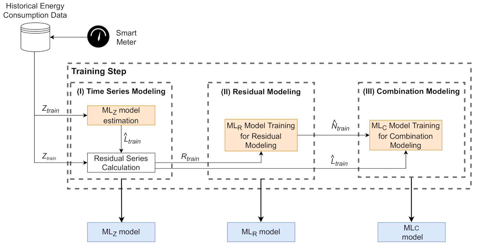
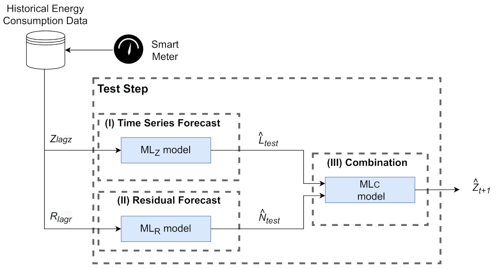
The proposed Evolutionary Hybrid System (EvoHyS) can be better understood by splitting into two steps: training and testing. Figure 1 and Figure 2 show that each step is divided into three phases. In the training step (Figure 1), the training set of the the time series ($Z_{train}$) is modeled by a linear model (ML${}_{\mathrm{Z}}$), an ML model (ML${}_{\mathrm{R}}$) is used in the modeling of the residual series ($E_{train}$), and the combination of the linear and non-linear estimates is performed with an ML model ((ML${}_{\mathrm{C}}$)). Figure 2 shows that the linear (ML${}_{\mathrm{Z}}$) and ML (ML${}_{\mathrm{R}}$) models are employed in the test step to forecast the time series and respective residuals. After that, the ML${}_{\mathrm{C}}$ model is used to combine these estimates, generating the final forecast.

Figure 1. Diagram of the training step of the Evolutionary Hybrid System (EvoHyS).

Figure 2. Diagram of the test step of the EvoHyS.

For linear modeling, a Seasonal Autoregressive Integrated Moving Average (SARIMA) model was chosen as ML${}_{\mathrm{Z}}$ due to its ability to model seasonal time series, such as historical energy consumption data. The Box & Jenkins methodology [14] used in the design and parameters adjust of the SARIMA model performs the modeling of the linear patterns presented in the training data (Equation (3)).

$${\widehat{L}}_{train}={\mathrm{ML}}_{\mathrm{Z}}\left(Z_{train}\right).$$

(3)

After ML${}_{\mathrm{Z}}$ model estimation, the residual series ($R_{train}$) is calculated from the difference between the training data ($Z_{train}$) and the linear forecast (${\widehat{L}}_{train}$) according to Equation (4),

$$R_{train}=Z_{train}-{\widehat{L}}_{train}.$$

(4)

Figure 1 shows that the outputs of Stage (I) of the training step are: the linear forecast (${\widehat{L}}_{train}$), the residual series ($R_{train}$), and the estimated SARIMA model (ML${}_{\mathrm{Z}}$). The SARIMA model is used in the test step.

Figure 1 shows that Stage (II) of the training step receives the residual series ($R_{train}$) as input data. In this stage, an ML technique (${\mathrm{ML}}_{\mathrm{R}}$) is trained to model the non-linear patterns that were not modeled in Stage (I). In this stage, $R_{train}$ is subdivided into training and validation sets to ML${}_{\mathrm{R}}$ parameters estimation. The Support Vector Regression (SVR) model was chosen to perform the non-linear modeling of the residual series. In contrast to ML models, such as neural networks, the SVR performs a quadratic optimization which yields a single minimal solution [57]. Furthermore, SVR models have shown accurate results in residual modeling [21]. A Genetic Algorithm (GA) is employed to search the SVR parameters and the best set of temporal lags. The objective is to improve the residual modeling using the ability of exploration and exploitation of the GA. The forecast of the non-linear patterns (${\widehat{N}}_{train}$) using the residual series ($R_{train}$) modeling is performed after the GA finds the parameters and the set of temporal lags that maximizes the accuracy of the SVR (Equation (5)).

$${\widehat{N}}_{train}=GA\left({\mathrm{ML}}_{\mathrm{R}}\left(R_{train}\right)\right).$$

(5)

The outputs of Stage (II) of the training step are the trained ${\mathrm{ML}}_{\mathrm{R}}$ and the forecast of the residuals (${\widehat{N}}_{train}$). The trained ${\mathrm{ML}}_{\mathrm{R}}$ is used in the Test Step.

Stage (III) of the training step employs an ML model (${\mathrm{ML}}_{\mathrm{C}}$) to search for the most suitable combination between the linear and non-linear forecasts. An MLP neural network was selected to perform the combination due to of its robustness against noise and the ability to approximate any non-linear function [58,59]. The definition of the inputs of the ${\mathrm{ML}}_{\mathrm{C}}$ is an important task [21] since it is closely related to the accuracy of the system. Thus, a GA is used to define the MLP parameters, such as the activation function, optimization algorithm, and number of hidden neurons. Equation (6) shows the final forecast in the training step of the EvoHyS.

$${\widehat{Z}}_{train}=GA\left({\mathrm{ML}}_{\mathrm{C}}({\widehat{L}}_{train},{\widehat{N}}_{train})\right).$$

(6)

Figure 1 shows that the output of the Stage (III) of the training step is the trained ${\mathrm{ML}}_{\mathrm{C}}$ model. In Stages (II) and (III), a validation set is employed for: verifying the ability of generalization of the ML models, avoiding the overfitting, and selecting the best hyperparameters setting. This validation set is a subset of the training set used in Stage (I) to estimate the parameters of the SARIMA model.

In the test step, as presented in Figure 2, the Stages (I) and (II) receive the test patterns of the time series ($Z_{lagz}$) and residual series ($R_{lagr}$), respectively. The number of time lags $lagz$ and $lagr$ used as inputs for the ${\mathrm{ML}}_{\mathrm{Z}}$ and ${\mathrm{ML}}_{\mathrm{R}}$ models were defined in the Stages (I) and (II) of the training step. In Stage (I), the ${\mathrm{ML}}_{\mathrm{Z}}$ model generates the time series forecast (${\widehat{L}}_{test}$), and in Stage (II) the ${\mathrm{ML}}_{\mathrm{R}}$ model generates the residual forecast (${\widehat{N}}_{test}$). Finally, in Stage (III), the ${\mathrm{ML}}_{\mathrm{C}}$ model performs the final forecast from the combination of the outputs of Stages (I) and (II) according to Equation (7).

$${\widehat{Z}}_{t+1}={\mathrm{ML}}_{\mathrm{C}}({\widehat{L}}_{l1},{\widehat{N}}_{l2}),$$

(7)

where ${\widehat{L}}_{l1}$ and ${\widehat{N}}_{l2}$ are the forecasts used in the combination stage defined by GA in Stage (III) of the training step. Algorithms 1 and 2 summarize the description of the training and test steps in algorithmic language.

Algorithm 1 Training Step

1: Input: $Z_{train}=[z_1,z_2,\dots ,z_{train}]$          training vector of size $train$ 2: Output: ${\mathrm{ML}}_{\mathrm{Z}},{\mathrm{ML}}_{\mathrm{R}},{\mathrm{ML}}_{\mathrm{C}}$                                       ▹ trained models 3: ML${}_{\mathrm{Z}}$← modelTraining($Z_{train}$)                                       ▹ Stage (I) 4: ${\widehat{L}}_{train}\leftarrow$ forecast(ML${}_Z$, $Z_{train}$) 5: $R_{train}\leftarrow (Z_{train}-{\widehat{L}}_{train})$ 6: ML${}_{\mathrm{R}}$← modelTraining($R_{train}$)                                               ▹ Stage (II) 7: ${\widehat{N}}_{train}\leftarrow$ forecast(ML${}_R$, $R_{train}$) 8: ML${}_{\mathrm{C}}$← modelTraining(${\widehat{L}}_{train}$,${\widehat{N}}_{train}$)                                  ▹ Stage (II) 9: ${\widehat{Z}}_{train}\leftarrow$ forecast(ML${}_C$,${\widehat{L}}_{train}$,${\widehat{N}}_{train}$)

Algorithm 2 Testing Step

1: Input: $Z_{lagz}$, $R_{lagr}$, ML${}_{\mathrm{Z}}$, ML${}_{\mathrm{R}}$, ML${}_{\mathrm{C}}$ 2: Output: ${\widehat{Z}}_{t+1}$ 3: ${\widehat{L}}_{test}\leftarrow$ forecast(ML${}_{\mathrm{Z}}$, $Z_{lagz}$)                                                ▹ Stage (I) 4: ${\widehat{N}}_{test}\leftarrow$ forecast(ML${}_{\mathrm{R}}$, $R_{lagr}$)                                                 ▹ Stage (I) 5: ${\widehat{Z}}_{t+1}\leftarrow$ forecast(ML${}_{\mathrm{C}}$,${\widehat{L}}_{l1}$,${\widehat{N}}_{l2}$)                                              ▹ Stage (I)

3.1. Genetic Algorithm

In a Genetic Algorithm (GA), a set of solutions (population) undergoes an evolutionary process inspired by Charles Darwin’s theory of evolution [60]. The evolution consists of changes in the characteristics of the population over generations guided by the fitness function. The genetic characteristics are passed to the next generation from the genetic operators (crossover and mutation). Natural selection (parent and survivor selection) improves the fitness of the population’s individuals over generations. The EvoHyS uses a GA in the Stages (II) and (III) of the training step (Figure 1). In Stages (II) and (III), the GA optimizes the ${\mathrm{ML}}_{\mathrm{R}}$ and ${\mathrm{ML}}_{\mathrm{C}}$ models, respectively.

The proposed GA can be described by defining four main components: Chromosome, Fitness Function, Reproduction (Crossover and Mutation), and Survivor Selection. Each one of these components will be described in the following sections.

3.1.1. Chromosome

In this work, the chromosome, or genotype, contains the models’ parameters to be optimized in Stages (II) and (III) of the training step (Figure 1). Figure 3 shows the generic representation of the chromosomes that codifies the ${\mathrm{ML}}_{\mathrm{R}}$ and ${\mathrm{ML}}_{\mathrm{C}}$ models. For both individuals, the chromosome is a fixed-length vector that contains two distinct parts. In the first block, there is information regarding lags that can be utilized as inputs for the model. Its size corresponds to the maximum number of lags that can be used by the model. Each position contains a binary value (0 or 1), which corresponds to a given lag’s absence or presence. In the second block the information regarding the parameters of the model is presented. A list of possible values is established for each model parameter, where each parameter search space is defined through different orders of magnitude or according to predefined choices present in popular machine learning libraries, such as scikit-learn [61]. The population is randomly generated in both Stages (II) and (III).

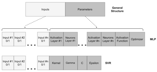
Figure 3. Chromossome of the individuals of the proposed algorithm.

In Stage (II), the SVR model is used as ${\mathrm{ML}}_{\mathrm{R}}$. For that, the chromosome’s first block is composed of time lags used for residual modeling. The second block holds information regarding the SVR parameters’ configuration, such as the kernel parameter gamma, the regularization factor C, and the $\epsilon$, which defines the $\epsilon$-sensitive cost function [57].

In Stage (III), the MLP model is employed as the combination mode, and is represented as ${\mathrm{ML}}_{\mathrm{C}}$. In the combination stage (Stage (III)), the first block consists of the input data employed to perform the final forecasting. The second part comprises genes that contain information regarding the hidden layer, activation function, and learning algorithm. The maximum number of hidden layers is previously defined. The number of neurons per layer, activation function, and learning algorithm are determined from a list of possible values. For each hidden layer, there is a binary value (0/1) that corresponds to the absence/presence of a given hidden layer.

3.1.2. Fitness Function

The fitness function used for the evaluation of each individual is given by Equation (8).

$$fitness=\frac{1}{1+MSE}$$

(8)

where

$$\mathrm{MSE}=\frac{1}{n}\sum {(Z_t-{\widehat{Z}}_t)}^2.$$

(9)

The Mean Squared Error (MSE) is obtained by the difference between the actual values and the forecast of the model. The validation set is used to evaluate the generalization ability of the forecasting model.

For the MLP model (Stage (III)), each individual is evaluated three times with different initialization of weights due to its stochastic nature. From those three evaluations, the best model is selected.

3.1.3. Reproduction

The next generation is created from current population from two ways. The first group consists of copies of the current population that are chosen using the roulette wheel selection. The process is performed with replacement, once the selected individual can be chosen again. The first group is generated until $(1-c_r)·P_{size}$, where $c_r$ and $P_{size}$ are the crossover rate previously defined in the interval [0, 1] and the size of the population, respectively.

Another group is created combining the genes of two parents chosen from roulette wheel selection. Each one of the offspring is produced from single-point crossover between selected two individuals. The process is performed with replacement until $c_r·P_{size}$.

The objective of the adopted strategy in the crossover is to enhance the chance of the fittest individuals remain in the population, accelerating the convergence of the algorithm. In addition, this reproduction aims to balance the trade-off between exploration and exploitation of the GA.

After crossover, all offspring is subject to mutations in their genes. The objective of that is to explore the search space and to guarantee the variability in the population. The number of mutations is chosen randomly for each individual of the offspring using a uniform distribution for a specific range, which can be defined as $[0,n_{max}]$. The initial value for the maximum number of mutations ($n_{max}$) is previously defined on the first iteration. For later iterations, $n_{max}$ increases one unit by epoch. As a result, while the population convergences, the proposed GA increases $n_{max}$ in order to keep adding variability, aiming to avoid premature convergence.

For binary genes, the mutation performs a reversion of the current state (from 0 to 1 or vice-versa). In other genes, the mutation replaces the current state with a new option chosen randomly from a list of possible states.

3.1.4. Survivor Selection

The offspring generated after the reproduction phase using genetic operators (crossover and mutation) has the same quantity of individuals as the previous population. Thus, the replacement of the population is performed without the need to have a survivor selection operator based on fitness. This replacement strategy aims to escape local minima that may occur in the previous iteration.

4. Experimental Evaluation

4.1. Setup

Data. Acquiring time series data is limited and challenging in the smart metering context since applications are performed in real buildings. The proposed hybrid system is evaluated taking into consideration the data collected by the smart grid infrastructure installed in a residential building [28] regarding the total hourly energy consumption between 2015 June 22 to 2015 July 26, totaling 2879 points. This same data set was used in the time series forecasting context by previous papers [4,7,28] for evaluation purposes.

The data set was split into training, validation, and testing samples following the temporal order, each one comprising 1706, 442, and 671 data points, respectively. The SARIMA model training was performed using the training and validation samples. The performance analysis was performed in the whole testing set and for each day of the week (Sunday, Monday, Tuesday, Wednesday, Thursday, Friday, and Saturday).

Selection of Parameters. The parameter selection for the components of the proposed hybrid system is performed in different ways for linear and non-linear models. SARIMA model is defined using the Box & Jenkins methodology [14]. The parameters of the SVR model are defined by GA according to the following value options described below:

• input_active = (0, 1)
• kernel = (linear, poly2, poly3, poly4, poly5, poly6, rbf, sigmoid)
• gamma = (scale, auto)
• C = (${10}^{-5}$, ${10}^{-4}$, ${10}^{-3}$, ${10}^{-2}$, ${10}^{-1}$, ${10}^0$, ${10}^1$, ${10}^2$, ${10}^3$, ${10}^4$)
• epsilon = (0.0, ${10}^{-5}$, ${10}^{-4}$, ${10}^{-3}$, ${10}^{-2}$, ${10}^{-1}$, ${10}^0$, ${10}^1$)

The $\mathrm{input}\_\mathrm{active}$ parameter assumes a binary value indicating the presence or absence of a given input, according to Figure 3. The $\mathrm{kernel}$ represents eight possible kernel functions: Linear, polynomial with degrees 2, 3, 4, 5, and 6; radial basis function (rbf) and sigmoid. Parameter C is a regularization factor and $\epsilon$ is used in the calculation of the error function.

The value for gamma is calculated according to the implementation of the machine learning library Scikit-learn [61] and SVR solver implementation libSVM [62] which allows two predefined possibilities, which are discussed by Braga et al. [63]:

• if gamma = auto, then the chosen value of gamma is defined as $1/n_{features}$, where $n_{features}$ represents the number of features in the input data,
• if gamma = scale, then the adopted value for gamma is $1/(n_{features}·{\sigma }^2)$ where $\sigma$ represents the standard deviation of the input data.

Regarding the MLP network, the possible values in the search space are:

• input_active = (0, 1)
• activation = (identity, logistic, tanh, relu)
• solver = (sgd, adam, lbfgs)
• layer_active = (0, 1)
• layer_nodes = (1, 2, 4, 8, 16, 32, 64, 128, 256, 512, 1024, 2048)

The activation represents the activation function, and can assume function, such as identity, logistic, hyperbolic tangent (tanh), and rectified linear unit (relu). The solver represents the algorithm used in the training process of the MLP. The number of hidden neurons of the MLP is defined through the $\mathrm{layer}\_\mathrm{nodes}$ parameter and each layer can be activated using a binary value of variable $\mathrm{layer}\_\mathrm{active}$.

Table 1 presents the selected models by GA from performance in the validation set. SVR with Radial Basis Function (RBF) kernel was the chosen residual model and the MLP used for the combination model only has 1 layer with 32 neurons. The column Lags presents the number of lags used by the models.

Table 1. Selected models by Genetic Algorithm (GA).

Model	Types	Parameters	Lags
ML${}_{\mathrm{R}}$	SVR	C = 0.01, epsilon = 1 $\times {10}^{-5}$, gamma = ‘scale’, kernel = ‘rbf’	1,5,8,9
ML${}_{\mathrm{C}}$	MLP	neurons = (32), activ. = ‘relu’,optim. = ‘adam’	Linear: 0,2,5,6,7; non-linear: 3,5,7,8

Baselines. The proposed hybrid system is compared with previous approaches, comprising single methods, ensembles, and hybrid methods. EvoHyS is compared to the models presented in the work of Chou and Tran [7]. For the single models, SARIMA, MLP, SVR, Long Short-term Memory neural network (LSTM), Linear regression (LR), and Classification and Regression Trees (C&R Tree) are considered. The ensemble methods employed consist of bagging of MLPs and an ensemble based on SVR and LR methods (SVR+LR). The hybrid systems used in the comparison are SARIMA-MetaFA-LSSVR and SARIMA-PSO-LSSVR. In both hybrid systems, the linear SARIMA model is employed in the time series forecasting. In SARIMA-MetaFA-LSSVR, the residual modeling is performed using a MetaFA-LSSVR. This step is performed using the residual series and exogenous data (temperature, day of the week, and hour of the day) to generate the energy consumption forecast [28]. The SARIMA-PSO-LSSVR system performs the residual modeling similarly to the aforementioned hybrid system using a Particle Swarm Optimization (PSO) to optimize the LSSVR parameters.

Evaluation Metrics. The models’ evaluation is performed with five error metrics: Correlation Coefficient (R), Mean Absolute Percentage Error (MAPE), Mean Absolute Error (MAE), Root Mean Squared Error (RMSE), and Maximum Absolute Error (MaxAE). The correlation coefficient (R) described in Equation (10) measures the linear dependencies between the actual ($Z_t$) and forecast series (${\widehat{Z}}_t$); thus, values of R closer to 1 indicate more accurate forecasts.

$$\mathrm{R}=\frac{\sum (Z_t-\overline{Z})(\widehat{Z_t}-\overline{\widehat{Z}})}{\sqrt{\sum {(Z_t-\overline{Z})}^2\sum (\widehat{Z_t}-\overline{\widehat{Z}})}}.$$

(10)

MAPE provides a percentage value over the errors in the forecasts. It has the advantage of being scale independent and easy to interpret. However, it is an asymmetric measure, showing a skewed distribution when $Z_t$ is close to zero. Furthermore, it penalizes forecasts that exceed the actual value ($Z_t$) [64]. MAPE is defined in Equation (11),

$$\mathrm{MAPE}=\frac{100}{n}\sum \left|\frac{Z_t-{\widehat{Z}}_t}{Z_t}\right|,$$

(11)

where n is the number of samples.

MAE, presented in Equation (12), offers an error evaluation in the same scale of the data and is less sensitive to outliers than quadratic error based metrics.

$$\mathrm{MAE}=\frac{1}{n}\sum \left|Z_t-{\widehat{Z}}_t\right|.$$

(12)

RMSE (Equation (13)) is an evaluation metric that promotes a heavier penalty on higher errors. It also presents the results on the same scale as the data. However, it is more sensitive to outliers than the MAE [64].

$$\mathrm{RMSE}=\sqrt{\frac{1}{n}\sum {(Z_t-{\widehat{Z}}_t)}^2}.$$

(13)

MaxAE (Equation (14)) indicates the maximum error in the occurrence of energy load peaks.

$$\mathrm{MaxAE}=max\left(\left|Z_t-{\widehat{Z}}_t\right|\right).$$

(14)

In order to directly compare the proposal with other methods, the percentage difference (PD) is calculated between the proposed hybrid system and literature models. Equations (15) and (16) show the percentage difference for RMSE, MAE, MAPE, and MaxAE measures ($PD$) and for R metric ($P{D}_R$), respectively.

$$PD=100\times \frac{Mode{l}_{LM}-Mode{l}_{PR}}{Mode{l}_{LM}},$$

(15)

$$P{D}_R=100\times \frac{Mode{l}_{PR}-Mode{l}_{LM}}{Mode{l}_{LM}},$$

(16)

where $Mode{l}_{PR}$ and $Mode{l}_{LM}$ are the metric of the EvoHyS and of the literature models, respectively. Positive values of $PD$ indicates an improvement of the proposed hybrid system, while negative values indicate that the proposal got worse results.

To perform a statistical comparison of the previous models with the proposed hybrid system, we apply the Diebold-Mariano hypothesis test [65]. The null hypothesis is that there is no significant difference with respect to the RMSE mean between the evaluated models. We consider a significance level of 0.05, which means that for p-values lower than 0.05 the null hypothesis is rejected.

4.2. Results

Table 2 presents the results for the five evaluation metrics for each day of the week attained by the proposed and literature methods. In general, the proposed hybrid system (EvoHyS) outperformed the previous approaches in several metrics for this scenario. More specifically, EvoHyS obtained the best values in 20 out of 35 cases, and the majority of them is on the RMSE, MAE, and MAPE metrics. This behavior is related to the MSE metric, which was used as a target function for the training of the proposed hybrid system.

Table 2. The performance of the EvoHyS and literature models in terms of Correlation Coefficient (R), Mean Absolute Percentage Error (MAPE), Mean Absolute Error (MAE), Root Mean Squared Error (RMSE), and Maximum Absolute Error (MaxAE) for each day of the week. The best values are highlighted in bold.

Approach	Model	Measure	Mon.	Tue.	Wed.	Thur.	Fri.	Sat.	Sun.	Max	Min
		R	0.192	0.519	0.332	0.602	0.733	0.527	0.138	0.733	0.138
		RMSE (kWh)	0.146	0.081	0.176	0.109	0.074	0.129	0.098	0.176	0.074
	SARIMA	MAE (kWh)	0.103	0.058	0.161	0.073	0.055	0.102	0.085	0.161	0.055
		MAPE (%)	49.79	26.23	103.20	47.52	34.01	80.35	82.53	103.20	26.23
		MaxAE (kWh)	0.180	0.226	0.983	0.265	0.178	0.204	0.213	0.983	0.178
		R	0.373	0.729	0.518	0.697	0.645	0.651	0.276	0.729	0.276
		RMSE (kWh)	0.097	0.068	0.116	0.105	0.073	0.068	0.116	0.116	0.068
	MLP	MAE (kWh)	0.058	0.045	0.068	0.083	0.051	0.052	0.044	0.083	0.044
		MAPE (%)	35.06	19.04	34.95	56.69	29.29	40.82	41.99	56.69	19.04
		MaxAE (kWh)	0.340	0.360	0.529	0.375	0.226	0.177	0.464	0.529	0.177
		R	0.339	0.371	0.345	0.725	0.535	0.584	0.19	0.725	0.19
		RMSE (kWh)	0.094	0.109	0.134	0.089	0.077	0.095	0.108	0.134	0.077
Single	SVR	MAE (kWh)	0.064	0.082	0.085	0.062	0.058	0.065	0.072	0.085	0.058
Model		MAPE (%)	34.78	37.25	34.53	36.96	34.76	49.67	74.62	74.62	34.53
		MaxAE (kWh)	0.308	0.371	0.526	0.335	0.215	0.279	0.276	0.526	0.215
		R	0.745	0.839	0.874	0.751	0.825	0.879	0.911	0.911	0.745
		RMSE (kWh)	0.052	0.050	0.058	0.052	0.042	0.044	0.047	0.058	0.042
	LSTM	MAE (kWh)	0.030	0.033	0.037	0.032	0.020	0.028	0.022	0.037	0.020
		MAPE (%)	14.18	13.74	16.71	16.81	11.65	14.84	12.28	16.81	11.65
		MaxAE (kWh)	0.307	0.239	0.308	0.289	0.310	0.166	0.318	0.318	0.166
		R	0.296	0.326	0.525	0.593	0.57	0.563	0.239	0.593	0.239
		RMSE (kWh)	0.099	0.103	0.109	0.111	0.105	0.063	0.119	0.119	0.063
	LR	MAE (kWh)	0.069	0.068	0.069	0.064	0.076	0.039	0.046	0.076	0.039
		MAPE (%)	42.62	28.15	37.32	42.89	51.92	22.79	43.93	51.92	22.79
		MaxAE (kWh)	0.348	0.363	0.390	0.390	0.355	0.264	0.655	0.655	0.264
		R	0.392	0.519	0.381	0.355	0.425	0.512	0.080	0.519	0.080
		RMSE (kWh)	0.097	0.103	0.125	0.116	0.099	0.124	0.087	0.125	0.087
	C&R Tree	MAE (kWh)	0.058	0.083	0.068	0.089	0.078	0.085	0.056	0.089	0.056
		MAPE (%)	35.06	40.41	26.47	65.49	48.96	63.43	57.61	65.49	26.47
		MaxAE (kWh)	0.409	0.262	0.538	0.347	0.327	0.346	0.305	0.538	0.262
		R	0.545	0.573	0.528	0.363	0.535	0.658	0.384	0.658	0.363
		RMSE (kWh)	0.087	0.131	0.126	0.167	0.362	0.101	0.174	0.362	0.087
Voting	SVR + LR	MAE (kWh)	0.048	0.064	0.058	0.056	0.178	0.171	0.153	0.178	0.048
		MAPE (%)	38.76	45.89	34.65	35.36	47.25	43.58	53.74	53.74	34.65
		MaxAE (kWh)	0.215	0.391	0.429	0.534	0.641	0.486	1.253	1.253	0.215
		R	0.551	0.616	0.658	0.623	0.734	0.651	0.416	0.734	0.416
		RMSE (kWh)	0.058	0.016	0.072	0.171	0.125	0.149	0.067	0.171	0.016
Bagging	MLP	MAE (kWh)	0.042	0.068	0.031	0.061	0.034	0.039	0.069	0.069	0.031
		MAPE (%)	34.82	54.95	38.19	35.31	28.07	42.62	62.19	62.19	28.07
		MaxAE (kWh)	0.277	0.549	0.157	0.232	0.451	0.381	0.319	0.549	0.157
		R	0.817	0.855	0.910	0.813	0.867	0.820	0.492	0.910	0.492
		RMSE (kWh)	0.179	0.180	0.180	0.170	0.172	0.168	0.100	0.180	0.100
	SARIMA-MetaFA-LSSVR	MAE (kWh)	0.032	0.032	0.032	0.029	0.030	0.028	0.010	0.032	0.010
		MAPE (%)	16.56	13.98	14.93	16.55	18.42	18.97	10.19	18.97	10.19
		MaxAE (kWh)	0.182	0.213	0.249	0.261	0.151	0.166	0.033	0.261	0.033
		R	0.731	0.632	0.845	0.908	0.867	0.825	0.493	0.908	0.493
Hybrid		RMSE (kWh)	0.240	0.239	0.182	0.180	0.171	0.162	0.100	0.240	0.100
System	SARIMA-PSO-LSSVR	MAE (kWh)	0.057	0.057	0.033	0.032	0.029	0.026	0.010	0.057	0.010
		MAPE (%)	33.85	22.45	14.28	14.95	18.00	17.40	10.20	33.85	10.20
		MaxAE (kWh)	0.240	0.458	0.234	0.244	0.151	0.182	0.033	0.458	0.033
		R	0.773	0.856	0.880	0.842	0.819	0.892	0.919	0.919	0.773
		RMSE (kWh)	0.049	0.048	0.056	0.042	0.042	0.043	0.045	0.056	0.042
	EvoHyS	MAE (kWh)	0.028	0.030	0.031	0.024	0.019	0.026	0.020	0.031	0.019
		MAPE (%)	14.36	13.12	13.99	12.60	11.80	12.04	11.27	14.36	11.27
		MaxAE (kWh)	0.326	0.236	0.302	0.277	0.315	0.190	0.302	0.326	0.190

Table 2 also shows the maximum and minimum values of the metrics over all data sets. EvoHyS achieved the best overall maximum values (Max), while the SARIMA-MetaFA-LSSVR obtained the overall best minimum values (Min).

Figure 4 shows the forecasting for the test set of the seven days of the week of the EvoHyS and SARIMA model. It can be seen that the EvoHyS was able to correct the SARIMA forecast for all cases of study.

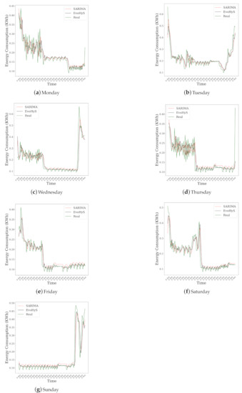
Figure 4. Forecasting for the test set of each day of the week with Seasonal Autoregressive Integrated Moving Average (SARIMA) and EvoHyS.

Table 3 shows the average values regarding all days of the week for the evaluation metrics. The results are calculated taking into consideration the values presented in Table 2. The proposed hybrid system achieved the best average results regarding all metrics except the MaxAE. The best average MaxAE was achieved by the SARIMA-MetaFA-LSSVR.

Table 3. The average values in terms of R, RMSE, MAE, MAPE, and MaxAE for EvoHyS and literature models. The best values are highlighted in bold.

Model	R	RMSE (kWh)	MAE (kWh)	MAPE (%)	MaxAE (kWh)
SARIMA	0.435	0.116	0.091	60.52	0.321
MLP	0.556	0.092	0.057	36.83	0.353
SVR	0.441	0.101	0.070	43.22	0.330
LSTM	0.832	0.049	0.029	14.32	0.277
LR	0.445	0.101	0.062	38.52	0.395
C&R Tree	0.381	0.107	0.074	48.20	0.362
SVR + LR	0.512	0.164	0.104	42.75	0.564
Bagging with MLPs	0.607	0.094	0.049	42.31	0.338
SARIMA-MetaFA-LSSVR	0.796	0.164	0.028	15.66	0.179
SARIMA-PSO-LSSVR	0.757	0.182	0.035	16.19	0.220
EvoHyS	0.854	0.046	0.025	12.74	0.278

Table 4 shows the percentage difference between the proposed hybrid system and the literature models for all evaluation metrics of the the average values shown in Table 3. For R, RMSE, MAE, MAPE, and MAxAE metrics, the greatest percentage differences were 124.25%, 74.51%, 75.63%, 78.95%, and 50.67% in relation to C&R Tree, SARIMA-PSO-LSSVR, SVR + LR, SARIMA, and SVR + LR, respectively. Only for the MaxAE metric, the proposed hybrid system obtained a negative percentage of −55.43% and −26.46% in comparison to the hybrid systems SARIMA-MetaFA-LSSVR and SARIMA- PSO-LSSVR, respectively. For R, RMSE, MAE, MAPE, and MAxAE metrics, the lowest percentage differences were 7.34% for SARIMA-MetaFA-LSSVR, 49.58% for MLP, 9.49% for SARIMA-MetaFA-LSSVR, 18.63% for SARIMA-MetaFA-LSSVR, and 13.33% for SARIMA.

Table 4. The percentage difference (%) between the proposed hybrid system (EvoHyS) and literature models according to Equations (15) and (16).

Model	R	RMSE (kWh)	MAE (kWh)	MAPE (%)	MaxAE (kWh)
SARIMA	96.41	60.01	72.15	78.95	13.33
MLP	53.67	49.58	55.54	65.41	21.18
SVR	93.74	54.07	63.79	70.53	15.69
LR	92.00	54.07	59.12	66.92	29.56
C&R Tree	124.25	56.64	65.75	73.57	23.14
SVR + LR	66.88	71.71	75.63	70.20	50.67
Bagging with MLPs	40.76	50.65	48.28	69.89	17.69
SARIMA-MetaFA-LSSVR	7.34	71.71	9.49	18.63	−55.43
SARIMA-PSO-LSSVR	12.87	74.51	27.59	21.30	−26.46

In order to perform a more robust comparison of the proposed hybrid system with the literature models, the Diebold-Mariano hypothesis test [66] was employed based on RMSE shown in Table 3. The hypothesis testing results are presented in Table 5, where p-values less than $0.05$ indicate a statistical difference between the methods at 95% confidence. The results show that the proposed hybrid system outperformed all the literature models, obtaining a statistically significant accuracy values.

Table 5. p-values of the Diebold-Mariano statistical test comparing the proposed hybrid system with the literature models.

Models	p-Value
SARIMA	$7.9\times {10}^{-5}$
MLP	$1.6\times {10}^{-6}$
SVR	$1.4\times {10}^{-10}$
LSTM	0.0087
LR	$1.2\times {10}^{-12}$
C&R Tree	$5.8\times {10}^{-17}$
SVR + LR	0.0259
Bagging with MLPs	0.0149
SARIMA-MetaFA-LSSVR	$3.9\times {10}^{-18}$
SARIMA-PSO-LSSVR	$1.2\times {10}^{-7}$

4.3. Discussion

In summary, the proposed hybrid system was compared with the single, ensembles, and hybrid models of the literature based on different error metrics in the context of energy consumption. The results presented in Table 2 show that the hybrid models achieved the best results in the energy consumption data sets for all days of the week, followed by ensemble models, such as Bagging, and single models, respectively.

Taking into consideration that traditional statistical models, such as SARIMA, present limited performance in the presence of non-linear patterns, and that non-linear models may not deal with linear and non-linear patterns equally well, the evaluation results show that hybrid systems in general outperformed single models. In Table 3, where the average values are compared, hybrid systems obtained the best overall values.

Among hybrid systems several strategies have been adopted. The proposed model is based on a three-stage architecture, where second and third stages are optimized by a Genetic Algorithm. The compared hybrid systems from the literature, namely the SARIMA-MetaFA-LSSVR and SARIMA-PSO-LSSVR which present a two-stage architecture, where the first performs linear modeling of the time series with the SARIMA model, and the second stage performs the non-linear modeling and combination together. The results obtained in Table 4 show that the proposed three-stage hybrid system could improve the results obtained by the other methods in most of the metrics, with the exception of the MaxAE.

The difference between accuracy of the models can be observed in Table 5, where the Diebold-Mariano hypothesis test was employed. The hypothesis test confirmed significant difference between the proposed model and the compared models.

5. Conclusions

The employment of smart meters has become an important alternative in monitoring energy consumption and efficiency, allowing better management and network planning. Forecasting energy consumption in smart meters have become an important tool for maintenance planning and fraud detection. However, achieving accurate forecasts may be a challenging task, since energy consumption data is likely to present linear and non-linear patterns [11].

In this work, an evolutionary hybrid system is proposed to forecast energy consumption in smart meters. In order to improve forecast accuracy, the proposed system (EvoHyS) is composed of three stages. First stage performs linear modeling through the employment of a SARIMA model. In the second stage, an evolutionary optimization based on a genetic algorithm is employed to find the best hyper-parameter of the SVR model, as well as to perform input selection. In the third and last stage, a combination of linear and non-linear models is performed using an MLP optimized by a genetic algorithm.

The experiments were conducted on data set of a smart grid network installed in a residential building. The simulations were carried considering the consumption per day of the week using several single and hybrid models proposed in the literature. In general, the EvoHyS achieved the best overall results, demonstrating good generalization performance on different days of the week.

The superior performance attained by EvoHyS compared with single models corroborates with previous studies [7,26,55] that show the benefits of using hybrid systems that combine statistical and ML models. The modeling of linear and non-linear patterns separately enables generating specialist models that combined achieve higher accuracy than single models. In comparison with literature hybrid systems (SARIMA-MetaFA-LSSVR and SARIMA-PSO-LSSVR), EvoHyS outperformed them in most evaluation measures. This result shows that employing an exclusive phase to combine linear and non-linear forecasts can improve hybrid systems’ accuracy in the smart meter consumption forecasting area.

The overall run-time complexity of the EvoHyS is the sum of the complexity of the three models used to perform the final prediction: SARIMA for time series forecast (linear on the number of lags), SVR with RBF kernel for the residual forecast (quadratic: number of lags times number of support vectors) and MLP (linear on the number of lags).

For future directions, an investigation of the influence on external variables, such as temperature, precipitation in energy consumption will be considered. The employment of deep learning forecasting methods in the proposed hybrid system architecture also may be analyzed. Furthermore, EvoHyS should be evaluated in other energy consumption scenarios that involve smart meters time series.

References

- El-hawary, M.E. The Smart Grid—State-of-the-art and Future Trends. Electr. Power Components Syst. 2014, 42, 239–250. [Google Scholar]
- Allouhi, A.; El Fouih, Y.; Kousksou, T.; Jamil, A.; Zeraouli, Y.; Mourad, Y. Energy consumption and efficiency in buildings: Current status and future trends. J. Clean. Prod. 2015, 109, 118–130. [Google Scholar]
- Zhao, H.X.; Magoulès, F. A review on the prediction of building energy consumption. Renew. Sustain. Energy Rev. 2012, 16, 3586–3592. [Google Scholar]
- Chou, J.S.; Ngo, N.T. Smart grid data analytics framework for increasing energy savings in residential buildings. Autom. Constr. 2016, 72, 247–257. [Google Scholar]
- Kolokotsa, D. The role of smart grids in the building sector. Energy Build. 2016, 116, 703–708. [Google Scholar]
- Cui, B.; ce Gao, D.; Wang, S.; Xue, X. Effectiveness and life-cycle cost-benefit analysis of active cold storages for building demand management for smart grid applications. Appl. Energy 2015, 147, 523–535. [Google Scholar]
- Chou, J.S.; Tran, D.S. Forecasting energy consumption time series using machine learning techniques based on usage patterns of residential householders. Energy 2018, 165, 709–726. [Google Scholar]
- Van Gerwen, R.; Jaarsma, S.; Wilhite, R. Smart metering. Leonardo-Energy Org. 2006, 9, 1–9. [Google Scholar]
- Fallah, S.N.; Deo, R.C.; Shojafar, M.; Conti, M.; Shamshirband, S. Computational Intelligence Approaches for Energy Load Forecasting in Smart Energy Management Grids: State of the Art, Future Challenges, and Research Directions. Energies 2018, 11, 596. [Google Scholar]
- Kabalci, Y. A survey on smart metering and smart grid communication. Renew. Sustain. Energy Rev. 2016, 57, 302–318. [Google Scholar]
- Chen, K.Y.; Wang, C.H. A hybrid SARIMA and support vector machines in forecasting the production values of the machinery industry in Taiwan. Expert Syst. Appl. 2007, 32, 254–264. [Google Scholar]
- Ding, N.; Benoit, C.; Foggia, G.; Bésanger, Y.; Wurtz, F. Neural network-based model design for short-term load forecast in distribution systems. IEEE Trans. Power Syst. 2015, 31, 72–81. [Google Scholar]
- Maldonado, S.; González, A.; Crone, S. Automatic time series analysis for electric load forecasting via support vector regression. Appl. Soft Comput. 2019, 83, 105616. [Google Scholar]
- Box, G.E.; Jenkins, G.M.; Reinsel, G.C.; Ljung, G.M. Time Series Analysis: Forecasting and Control; John Wiley & Sons: Hoboken, NJ, USA, 2015. [Google Scholar]
- De Gooijer, J.G.; Hyndman, R.J. 25 years of time series forecasting. Int. J. Forecast. 2006, 22, 443–473. [Google Scholar]
- Ferreira, V.H.; da Silva, A.P.A. Toward estimating autonomous neural network-based electric load forecasters. IEEE Trans. Power Syst. 2007, 22, 1554–1562. [Google Scholar]
- Elattar, E.E.; Goulermas, J.; Wu, Q.H. Electric load forecasting based on locally weighted support vector regression. IEEE Trans. Syst. Man Cybern. Part C Appl. Rev. 2010, 40, 438–447. [Google Scholar]
- Lu, J.C.; Niu, D.X.; Jia, Z.Y. A study of short-term load forecasting based on ARIMA-ANN. In Proceedings of the 2004 International Conference on Machine Learning and Cybernetics (IEEE Cat. No. 04EX826), Shanghai, China, 26–29 August 2004; Volume 5, pp. 3183–3187. [Google Scholar]
- Zhang, G.P. Time series forecasting using a hybrid ARIMA and neural network model. Neurocomputing 2003, 50, 159–175. [Google Scholar]
- Khashei, M.; Bijari, M. A novel hybridization of artificial neural networks and ARIMA models for time series forecasting. Appl. Soft Comput. 2011, 11, 2664–2675. [Google Scholar]
- Domingos, S.D.O.; de Oliveira, J.F.; de Mattos Neto, P.S. An intelligent hybridization of ARIMA with machine learning models for time series forecasting. Knowl.-Based Syst. 2019, 175, 72–86. [Google Scholar]
- de Mattos Neto, P.S.; de Oliveira, J.F.L.; Júnior, D.S.D.O.S.; Siqueira, H.V.; Marinho, M.H.D.N.; Madeiro, F. A Hybrid Nonlinear Combination System for Monthly Wind Speed Forecasting. IEEE Access 2020, 8, 191365–191377. [Google Scholar]
- Pai, P.F.; Lin, C.S. A hybrid ARIMA and support vector machines model in stock price forecasting. Omega 2005, 33, 497–505. [Google Scholar]
- Panigrahi, S.; Behera, H. A hybrid ETS–ANN model for time series forecasting. Eng. Appl. Artif. Intell. 2017, 66, 49–59. [Google Scholar]
- de Oliveira, J.F.; Ludermir, T.B. A hybrid evolutionary decomposition system for time series forecasting. Neurocomputing 2016, 180, 27–34. [Google Scholar]
- do Nascimento Camelo, H.; Lucio, P.S.; Leal Junior, J.B.V.; de Carvalho, P.C.M.; von Glehn dos Santos, D. Innovative hybrid models for forecasting time series applied in wind generation based on the combination of time series models with artificial neural networks. Energy 2018, 151, 347–357. [Google Scholar]
- Taskaya-Temizel, T.; Casey, M.C. A comparative study of autoregressive neural network hybrids. Neural Netw. 2005, 18, 781–789. [Google Scholar]
- Chou, J.S.; Ngo, N.T. Time series analytics using sliding window metaheuristic optimization-based machine learning system for identifying building energy consumption patterns. Appl. Energy 2016, 177, 751–770. [Google Scholar]
- Ahmad, T.; Chen, H. A review on machine learning forecasting growth trends and their real-time applications in different energy systems. Sustain. Cities Soc. 2020, 54, 102010. [Google Scholar]
- Deb, C.; Zhang, F.; Yang, J.; Lee, S.E.; Shah, K.W. A review on time series forecasting techniques for building energy consumption. Renew. Sustain. Energy Rev. 2017, 74, 902–924. [Google Scholar]
- Heydari, A.; Keynia, F.; Garcia, D.A.; De Santoli, L. Mid-Term Load Power Forecasting Considering Environment Emission using a Hybrid Intelligent Approach. In Proceedings of the 2018 5th International Symposium on Environment-Friendly Energies and Applications (EFEA), Rome, Italy, 24–26 September 2018; pp. 1–5. [Google Scholar]
- Chan, S.C.; Tsui, K.M.; Wu, H.C.; Hou, Y.; Wu, Y.; Wu, F.F. Load/Price Forecasting and Managing Demand Response for Smart Grids: Methodologies and Challenges. IEEE Signal Process. Mag. 2012, 29, 68–85. [Google Scholar] [CrossRef]
- Culaba, A.B.; Del Rosario, A.J.R.; Ubando, A.T.; Chang, J.S. Machine learning-based energy consumption clustering and forecasting for mixed-use buildings. Int. J. Energy Res. 2020, 44, 9659–9673. [Google Scholar]
- Gao, Y.; Ruan, Y.; Fang, C.; Yin, S. Deep learning and transfer learning models of energy consumption forecasting for a building with poor information data. Energy Build. 2020, 223, 110156. [Google Scholar]
- Pinto, T.; Praça, I.; Vale, Z.; Silva, J. Ensemble learning for electricity consumption forecasting in office buildings. Neurocomputing 2021, 423, 747–755. [Google Scholar]
- Walther, J.; Weigold, M. A Systematic Review on Predicting and Forecasting the Electrical Energy Consumption in the Manufacturing Industry. Energies 2021, 14, 968. [Google Scholar]
- Barzola-Monteses, J.; Espinoza-Andaluz, M.; Mite-León, M.; Flores-Morán, M. Energy Consumption of a Building by using Long Short-Term Memory Network: A Forecasting Study. In Proceedings of the 2020 39th International Conference of the Chilean Computer Science Society (SCCC), Coquimbo, Chile, 16–20 November 2020; pp. 1–6. [Google Scholar]
- Rana, M.; Koprinska, I. Forecasting electricity load with advanced wavelet neural networks. Neurocomputing 2016, 182, 118–132. [Google Scholar]
- Zolfaghari, M.; Golabi, M.R. Modeling and predicting the electricity production in hydropower using conjunction of wavelet transform, long short-term memory and random forest models. Renew. Energy 2021, 170, 1367–1381. [Google Scholar]
- El-Hendawi, M.; Wang, Z. An ensemble method of full wavelet packet transform and neural network for short term electrical load forecasting. Electr. Power Syst. Res. 2020, 182, 106265. [Google Scholar]
- Gajowniczek, K.; Ząbkowski, T. Short term electricity forecasting using individual smart meter data. Procedia Comput. Sci. 2014, 35, 589–597. [Google Scholar]
- Zhukov, A.V.; Sidorov, D.N.; Foley, A.M. Random forest based approach for concept drift handling. In Proceedings of the International Conference on Analysis of Images, Social Networks and Texts, Yekaterinburg, Russia, 7–9 April 2016; pp. 69–77. [Google Scholar]
- Heydari, A.; Nezhad, M.M.; Pirshayan, E.; Garcia, D.A.; Keynia, F.; De Santoli, L. Short-term electricity price and load forecasting in isolated power grids based on composite neural network and gravitational search optimization algorithm. Appl. Energy 2020, 277, 115503. [Google Scholar]
- Heydari, A.; Garcia, D.A.; Keynia, F.; Bisegna, F.; Santoli, L.D. Hybrid intelligent strategy for multifactor influenced electrical energy consumption forecasting. Energy Sources Part B Econ. Plann. Policy 2019, 14, 341–358. [Google Scholar]
- Yu, C.N.; Mirowski, P.; Ho, T.K. A sparse coding approach to household electricity demand forecasting in smart grids. IEEE Trans. Smart Grid 2016, 8, 738–748. [Google Scholar]
- Fekri, M.N.; Patel, H.; Grolinger, K.; Sharma, V. Deep learning for load forecasting with smart meter data: Online Adaptive Recurrent Neural Network. Appl. Energy 2021, 282, 116177. [Google Scholar]
- Li, L.; Meinrenken, C.J.; Modi, V.; Culligan, P.J. Short-term apartment-level load forecasting using a modified neural network with selected auto-regressive features. Appl. Energy 2021, 287, 116509. [Google Scholar]
- Komatsu, H.; Kimura, O. Peak demand alert system based on electricity demand forecasting for smart meter data. Energy Build. 2020, 225, 110307. [Google Scholar]
- Lusis, P.; Khalilpour, K.R.; Andrew, L.; Liebman, A. Short-term residential load forecasting: Impact of calendar effects and forecast granularity. Appl. Energy 2017, 205, 654–669. [Google Scholar]
- Sajjad, M.; Khan, Z.A.; Ullah, A.; Hussain, T.; Ullah, W.; Lee, M.Y.; Baik, S.W. A novel CNN-GRU-based hybrid approach for short-term residential load forecasting. IEEE Access 2020, 8, 143759–143768. [Google Scholar]
- Wang, Y.; Gan, D.; Sun, M.; Zhang, N.; Lu, Z.; Kang, C. Probabilistic individual load forecasting using pinball loss guided LSTM. Appl. Energy 2019, 235, 10–20. [Google Scholar]
- Zhang, L.; Wen, J.; Li, Y.; Chen, J.; Ye, Y.; Fu, Y.; Livingood, W. A review of machine learning in building load prediction. Appl. Energy 2021, 285, 116452. [Google Scholar]
- Somu, N.; Raman M R, G.; Ramamritham, K. A deep learning framework for building energy consumption forecast. Renew. Sustain. Energy Rev. 2021, 137, 110591. [Google Scholar]
- Chou, J.S.; Truong, D.N. Multistep energy consumption forecasting by metaheuristic optimization of time-series analysis and machine learning. Int. J. Energy Res. 2021, 45, 4581–4612. [Google Scholar]
- Chou, J.S.; Truong, D.N. A novel metaheuristic optimizer inspired by behavior of jellyfish in ocean. Appl. Math. Comput. 2021, 389, 125535. [Google Scholar]
- Bouktif, S.; Fiaz, A.; Ouni, A.; Serhani, M. Multi-sequence LSTM-RNN deep learning and metaheuristics for electric load forecasting. Energies 2020, 13, 391. [Google Scholar]
- Smola, A.J.; Schölkopf, B. A tutorial on support vector regression. Stat. Comput. 2004, 14, 199–222. [Google Scholar]
- Zhang, G.P. An investigation of neural networks for linear time-series forecasting. Comput. Oper. Res. 2001, 28, 1183–1202. [Google Scholar]
- Zhang, G.; Patuwo, B.; Hu, M.Y. A simulation study of artificial neural networks for nonlinear time-series forecasting. Comput. Oper. Res. 2001, 28, 381–396. [Google Scholar]
- Holland, J.H. Genetic algorithms and the optimal allocation of trials. SIAM J. Comput. 1973, 2, 88–105. [Google Scholar]
- Pedregosa, F.; Varoquaux, G.; Gramfort, A.; Michel, V.; Thirion, B.; Grisel, O.; Blondel, M.; Prettenhofer, P.; Weiss, R.; Dubourg, V.; et al. Scikit-learn: Machine learning in Python. J. Mach. Learn. Res. 2011, 12, 2825–2830. [Google Scholar]
- Chang, C.C.; Lin, C.J. LIBSVM: A library for support vector machines. ACM Trans. Intell. Syst. Technol. (TIST) 2011, 2, 1–27. [Google Scholar]
- Braga, I.; do Carmo, L.P.; Benatti, C.C.; Monard, M.C. A note on parameter selection for support vector machines. In Proceedings of the Mexican International Conference on Artificial Intelligence, México, Mexico, 24–30 November 2013; pp. 233–244. [Google Scholar]
- Hyndman, R.J.; Koehler, A.B. Another look at measures of forecast accuracy. Int. J. Forecast. 2006, 22, 679–688. [Google Scholar]
- Diebold, F.X.; Mariano, R.S. Comparing predictive accuracy. J. Bus. Econ. Stat. 2002, 20, 134–144. [Google Scholar]
- Harvey, D.; Leybourne, S.; Newbold, P. Testing the equality of prediction mean squared errors. Int. J. Forecast. 1997, 13, 281–291. [Google Scholar]
Publisher’s Note: MDPI stays neutral with regard to jurisdictional claims in published maps and institutional affiliations. |
© 2021 by the authors. Licensee MDPI, Basel, Switzerland. This article is an open access article distributed under the terms and conditions of the Creative Commons Attribution (CC BY) license (http://creativecommons.org/licenses/by/4.0/).