Abstract
Solar radiation homogenizers are multi-mirror devices that try to reshape the solar radiation distribution coming from a concentrator, so that, after passing through the homogenizer, the light flux becomes as much evenly distributed as possible. The optical behavior of these multi-reflective devices is complex and still ill-understood. The geometry of the concentrator defines the features of the concentrated flux and then the characteristics of a particular homogenizer must be chosen according to the envisaged use. In this work, we developed and used optical ray-tracing software to investigate how the homogenizer’s optical output is affected by the following homogenizer’s characteristics: (i) Number of reflecting surfaces; (ii) total length; (iii) position (relative to focal plane); and (iv) tilt angle (inclination) of reflecting surfaces. The obtained results provide valuable information for the use of these optical devices and may contribute to the development of more efficient strategies for homogenization of concentrated radiation generated by high-flux solar furnaces.
1. Introduction
In high-flux solar concentration systems, the flux of solar radiation that reaches the target is non-homogeneous, as discussed in our previous modelling work [1,2] and illustrated by considerable experimental evidence. Therefore, to expand the application field of solar-driven high-temperature technologies it is essential to improve the temperature homogeneity conditions, because for many applications, it is important to obtain a radiation distribution as homogeneous as possible over the working area [3]. For processing of (solid) bulk materials at the industrial scale (e.g., firing of ceramics, heat treatment of metallic parts, furnaces for glass melting or for glass fritting, calcination furnaces, etc.) it is indispensable that temperature control and temperature homogeneity conditions are guaranteed.
The so-called “radiation flux homogenizers” used by some researchers [4,5,6,7,8,9,10,11] are multi-reflective devices (with mirrored sides) designed to reshape the solar radiation flux coming from a concentrator so that, after passing through the homogenizer, the flux becomes as much evenly distributed as possible; i.e., homogenizers are optical devices aiming to increase the homogeneity of the distribution of flux, and they need to be studied in depth, together with other strategies for overcoming the problem of thermal inhomogeneity [12,13].
Until now, almost all the so-called “solar furnaces” are point-focusing solar concentration facilities. These high-flux solar furnaces are located throughout the world at universities, research institutes, and companies, operating at concentrations relevant to solar thermochemistry, materials processing, and thermal treatments [3]. Figure 1 shows a typical diagram of a typical high-flux solar furnace. This type of furnaces usually consists of: (i) A flat solar-tracking heliostat (or a group/field of heliostats); (ii) a parabolic collector mirror (which concentrates the solar flux); (iii) an attenuator or shutter (that allows reductions in the flux to control it); and (iv) a test zone located at the concentrator focus. The flat mirror(s) of the heliostat (or heliostats) reflects the (quasi) parallel solar beams onto the reflective surfaces of the parabolic concentrator, which in turn reflects them onto the test area. The inclination of the blades at the shutter (between the heliostat and the concentrator) regulates the amount of sunlight passing through them and therefore controls the solar flux incident on the concentrator. In solar furnaces, the test table is movable in three directions (East–West, North–South, up and down) thus allowing to place the test samples at a chosen location (near the high-concentration zone, but not necessarily at the focus). When necessary, a 45°-tilted flat mirror (not shown in Figure 1) may be placed at a certain distance between the concentrator and the focal point in order to reflect vertically the solar radiation so that the concentrated solar beam becomes vertically oriented [1,2].
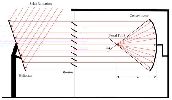
Figure 1.
Typical configuration of a high-flux solar furnace, showing its main components: The heliostat, the shutter, and the concentrator (α is the rim angle; L is the focal length i.e., the distance between the center of the parabolic concentrator and the theoretical focal point).
For this work, we improved our own ray tracing software (named LAM, Light Analysis Modelling) [1,2] to model the radiation output for several different homogenizers, with different geometries and operating conditions. The software works thus as a laboratory to study homogenizers, allowing us to learn as much as possible about these devices. The ultimate goal is to optimize the homogenizer geometry and position for a specific high-flux solar furnace. The purpose of the study is not to investigate the input radiation at the entrance of the homogenizer, generated by the concentrator, so this is kept constant for all simulations.
2. Computational Details
2.1. Radiation
Throughout this work we assume that the input radiation is formed by random parallel rays coming from a heliostat, that are subsequently concentrated by a paraboloid concentrator [1,2]. To imitate the radiation coming from the heliostat, we generate random points inside a circle with the same area of the projected paraboloid concentrator (see Figure 2). Parallel rays coming from these random points travel to the concentrator where they are reflected by specular reflection, moving then towards the paraboloid theoretical focal point, where they meet the homogenizer. To make our model more realistic, we use data based on a real solar furnace, the SF60 solar furnace available at Plataforma Solar de Almeria, Spain [14]. Therefore, throughout this work, we assume that the focal distance of the paraboloid concentrator is L = 7450 mm and the rim angle is α = 38°. Nonetheless, the results reported here should be valid for other solar furnace layouts.
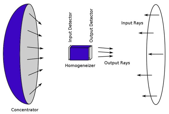
Figure 2.
General modelling layout used in this work: Random parallel rays generated in a circle equivalent to the projected concentrator, are reflected by the concentrator to the focal zone, where they are successively reflected inside the homogenizer. The whole experiment is monitored by detectors positioned immediately before and after the homogenizer.
In a mathematically perfect model, with a parabolic mirror, light rays are focused on a single focal point. In large scale solar furnaces, due to the inevitable local inaccuracies, this focal point is always replaced by a non-negligible focal circle. To fit our geometrical light models to reality, we scramble the radiation coming from the paraboloid, to achieve the focal diameter experimentally measured. In this work we assume a focal diameter of 250 mm (a typical value for this type of large-scale solar furnace).
For each light ray, coming from a position r0, with a direction defined by a wave vector k0, we construct an orthonormal basis, with unit vectors a1, a2, a3, with a3 pointing in the k0 direction. We can randomly change the ray position r0 or the ray orientation k0.
To scramble the position of r0 we generate a random point in a circle with some maximum radius rM, in cylindrical coordinates, r, φ, then convert to Cartesian coordinates x, y, then multiply by vectors a1, a2, to obtain a shift vector, in a plane perpendicular to k0, which is added to r0 to obtain the new scrambled position r1.
To scramble the orientation of k0 we generate a random position on a spherical surface with radius k0, in spherical coordinates, θ, φ, for some maximum polar angle θM (see reference [1] for details), then convert to Cartesian coordinates x, y, z, then multiply by vectors a1, a2, a3, to obtain the new vector k1, slightly rotated from the initial k0. For the solar furnace layout under consideration, the focal diameter of 250 mm can be achieved scrambling r0 with rM = 110 mm or scrambling k0 with θM = 0.8°. Throughout this work we used always the scrambling k0 technique because we think it is much closer to physical reality.
In all experiments reported in this work, we used 108 (hundred million) input light rays to collect the output data. Table 1 shows the input and output radiation coefficient-of-variation CV values (the most relevant results calculated in this work) for the default homogenizer conditions (4-side, 350-mm long, position 0, tilt angle 0°, as it will be reported later), as a function of the number of random rays generated. These tests show that: (1) For a number of rays smaller than 108 the radiation distributions are still far from convergence; (2) for a larger number of rays the much longer computation times do not seem to increase the fundamental quality of the results.

Table 1.
Model dependence on the number of input rays.
We also tested the influence of the sequences of random numbers (determined by the random seed) in the final results. Table 2 shows the same calculations for the default conditions, with 108 rays, as a function of the random seed. These tests show that the choice of random number sequences does not affect the results.
Table 2.
Model dependence on the random number sequences.
2.2. Homogenizers
By construction reasons, homogenizers used in high-flux solar furnaces should be simple, with flat reflective surfaces or a cylinder mirrored inside, with a behavior similar to a symmetric polygon with infinite faces. These devices can therefore be modelled by sets of flat, convex, polygons, as commonly used in computer graphics, to simplify mathematics. A flat polygon has always two faces, that can be distinguished entering the vertices sequentially, so one face will be clockwise oriented and the other will be counter-clockwise oriented.
In the software written for this work (see Figure 3a), it is always assumed that counter-clockwise oriented (internal) faces reflect the radiation (by specular reflection) while clockwise oriented (external) faces just lose the radiation (by diffuse reflection, scattering and absorption mechanisms).
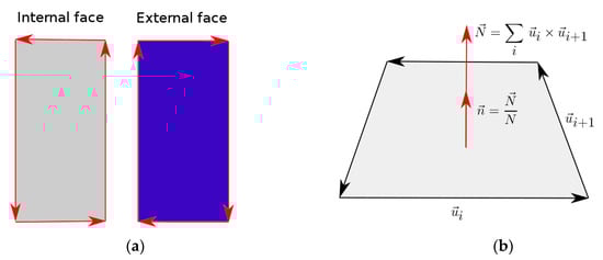
Figure 3.
(a) Counter-clockwise oriented face (left): Inside, reflective surface. Clockwise oriented face (right): Outside, non-reflective surface. Every flat convex polygon has two faces, which can be distinguished by the orientation of the ordered vertices; (b) adding the cross vectors between successive polygon edge vectors is a simple and robust way to compute a perpendicular vector N, which can then be normalized, dividing by its length. The polygon must be flat, convex, and the vertices must be ordered.
To obtain a point c (the polygon center, in highly symmetric polygons, such as those used in this work) inside an arbitrary (flat, convex) polygon, we can sum the vertices positions and divide by its number.
To obtain the normal unit vector n pointing outwards from the front (reflective) surface, we scan sequentially the polygon vertices to construct the corresponding edge vectors (see Figure 3b). Calculating the cross product of an edge vector with the next one, repeating for all edge vectors and summing everything, will produce a perpendicular vector, going outwards from the counter-clockwise face, that can then be normalized.
Knowing a point c in the polygon plane and its perpendicular vector n, we can calculate the point r1 where the input light ray (defined by a starting point r0 and a wave vector k0) intercepts the polygon plane (see ref. [1]).
To know whether the point r1 is inside or outside the polygon, we construct vectors from the point r1 to all the polygon vertices, in sequential, increasing order (see Figure 4). Calculating the cross product of each of these vectors with the next one, one of two things can happen: (1) all cross product vectors point in the same direction (the dot product between them is always positive), implying that r1 is inside the polygon; (2) not all cross points point in the same direction (at least one of the dot products is negative), implying that r1 is outside the polygon.
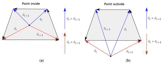
Figure 4.
(a) Point inside the polygon: The cross product between adjacent vectors going from the intersection point to the successive polygon vertices point always in the same direction. (b) Point outside the polygon: the cross product between adjacent vectors going from the intersection point to the successive polygon vertices point in opposite directions. In both cases, the polygon must be flat, convex, and the intersection point must be in the polygon plane.
In this work, we built five polygon-based homogenizers (see Table 3), with 3, 4, 6, 8, and 4 × 4 = 16 reflecting faces, following the conventions indicated above. Increasing the number of faces, the geometry tends to an open cylinder, reflecting inside, so we also modelled the cylinder homogenizer.
Table 3.
Radiation flux at homogenizer entrance and exit, as a function of the number of faces, for the following conditions: Total length = 350 mm; position = 0 (centered at the theoretical focal point), tilt angle = 0°.
To build the homogenizers, we used the following criterion for the lateral dimensions: the homogenizers are always centered along the concentrator axis, with an aperture as large as possible, without exceeding the 250 × 250 mm square area (the focal diameter for the scrambled radiation is 250 mm). For the 4-side homogenizer we used a 250 × 250 mm open channel. For the 4 × 4 homogenizer we used four 124 × 124 mm open channels, with a 2 mm thick wall separating them in both directions. For the cylinder homogenizer we used a diameter of 250 mm. For the 3-side homogenizer, the distance from the center to the vertices is 125 mm. Of course, we could have increased the triangle aperture, just moving it off the axis, but this would result in more complex, unbalanced, output patterns. For the 6-side homogenizer, the distance from the center to the vertices is also 125 mm. For the 8-side homogenizer, the distance from the center to the faces is 125 mm.
The input power can be increased simply enlarging the homogenizer aperture, increasing the device lateral dimensions, but this decreases the number of reflections inside and makes the device less efficient (and more cumbersome).
Using the same geometrical data, we also prepared masks, filtering radiation that fall outside the homogenizers overture, to facilitate analysis and to fit better the experimental conditions (this is the computational equivalent of covering all around the top entrance of each homogenizer with alumina, to protect the lateral faces against radiation damage).
When a ray of light intercepts a set of reflecting polygons, such as the five flat surface homogenizers studied in this work, the following algorithm is used: for each polygon, test if the ray intercepts the polygon plane, and then if the ray intersects the polygon inside. When the answer is no, just move to the next polygon. When the answer is yes, determine the distance from the ray starting point to the polygon intersection point, and compare with previous polygons, to determine the closest intersection point. After scanning all polygons, one of three things can happen: (1) No polygon was intersected, so the ray leaves the polygon-based device. This is the normal exit; (2) a back (non-reflecting) face was intersected, so the ray is discarded; (3) a front (reflecting) face was intersected, so the new reflected ray is calculated (see [1]). The new ray goes then through the same polygon-scanning procedure applied to the previous ray, and the process is repeated until case 1 (good exit) or case 2 (bad exit) occur.
For the cylinder homogenizer: (1) Rays intersecting the cylinder lateral surface are discarded; (2) rays not going through the overture just pass the cylinder (in this work we use a mask to trap them); (3) rays going inside are successively reflected by the inner cylinder surface until the output overture is reached, using an algorithm similar to the one described above for the flat surfaces homogenizers.
2.3. Detectors
A LAM detector is a rectangle of pixels (as an LCD screen), forming a 2D histogram where each pixel accumulates the number and length of rays (the radiation flux) intersecting that pixel during the experiment. By default, each pixel in a screen detector represents an area of 1 mm × 1 mm, and the number of rays hitting each pixel can be seen as a measure of flux, given for example in W/mm2, multiplied by some scaling factor. Multiplying this flux by the 1 mm2 unit area we obtain the same number for the power in W received by each pixel. Summing for all illuminated pixels in the detector, we obtain the total power received by the detector. The scaling factor can be calculated, for example to compare with experimental data, dividing the number of non-concentrated input rays (coming from the heliostat) by the circle area where they were generated (so we get the number of rays/mm2). This ratio multiplied by the scaling factor can be made equal to the locally measured solar flux (usually around 1.0 kW/m2 = 1.0 mW/mm2, smaller than 1.36 kW/m2, the raw sun radiation flux).
As a photographic camera, a LAM detector is determined by its center, its pointing direction, and its up direction. After the experiment, the data collected can be used to: (1) Produce statistical information (flux mean value, standard deviation, coefficient of variation (CV), minimum and maximum values, total power, etc.) above a given baseline (so non illuminated regions are discarded); (2) create profile graphs of accumulated radiation flux along any line in the 2D detector rectangle; (3) generate color images of radiation flux for the detector rectangle.
LAM supports several different color schemes to represent the accumulated data, usually going from a blue color for the lowest accumulated value (above the baseline), to a red color for the highest accumulated value. Non illuminated pixels, with values below the baseline, are usually colored black. LAM supports a relative color scheme, where minimum (blue) and maximum (red) values are automatically determined for each image, and an absolute color scheme, where minimum (blue) and maximum (red) values are previously specified by the user. The absolute scheme allows direct comparison of different images but tends to reduce the range of colors used in each image, thus hiding valuable pattern details. For example, an image collected close to the focal plane will be mostly red, while an image collected far from the focal plane will be mostly blue. In this work we chose the relative approach, which gives us a maximum of color information for each image, although this means that colors cannot be directly compared between different images. The same red pixel in two different images might represent flux values completely different.
3. Results and Discussion
3.1. Influence of Number of Reflecting Surfaces
Table 4 summarizes the main numeric results of the computer simulations carried out using LAM on the five polygon-based homogenizers as well as on the cylinder homogenizer. For comparing the influence of the number of reflecting surfaces, the total length of each of the homogenizers were kept constant and equal to 350 mm. The homogenizer position was also kept constant, with the geometric center of each device positioned at the theoretical focal point of the radiation coming from the concentrator. The coefficient of variation (CV) of the radiation flux is a good parameter to assess the degree of flux homogeneity. Total power at the entrance (input) and at the exit (output) of each of the homogenizers is expressed in terms of number of ray counts (given by the LAM detectors). Perfect match between input and output power values reveals that incoming rays suffer specular reflection inside the homogenizer and all of them exit at the other end of the homogenizer.
Table 4.
CV and power at homogenizer entrance and exit, as a function of the number of faces, for the following conditions: Total length = 350 mm; position = 0 (centered at the theoretical focal point), tilt angle = 0°.
Analyzing the results included in Table 4, the first conclusion we can derive is an enormous decrease in the CV, from the input to the output radiation, for all geometries included in this study. These devices are difficult to construct and easy to destroy, but these results seem to justify its use. We may also conclude that an increase in the number of reflecting surfaces does not contribute towards an increase in homogeneity at the exit (output) of the homogenizer. Comparing the radiation-flux CV values, the four faces/square homogenizer is undoubtedly the most suitable one, showing the lowest value of output radiation CV and the highest value of power. This is good news because these four-face devices are easier to build than its counterparts with more faces and are less prone to junction failure at high temperature. Most homogenizers currently used in high-flux solar furnaces are four-face devices.
3.2. Influence of Homogenizer Length
Considering only four-face homogenizers, all of them with the same square cross section and all of them with their geometrical center located at the focal point, we have studied the influence of the homogenizer length. For this study, we have compared the results obtained in homogenizers with the following lengths: 250, 300, 350, 400, 450, and 500 mm (see Table 5). Homogenizers shorter than 250 mm are ineffective and are not used in high-flux solar facilities, because the number of reflections inside is too small to make a difference.
Table 5.
Radiation flux, CV, and power at homogenizer entrance and exit, as a function of the total length, for the following conditions: Number of faces = 4; position = 0 (centered at the theoretical focal point), tilt angle = 0°.
From the results presented in Table 5, it is clear that an increase in the length of the homogenizer leads to a decrease in the transmitted power, because when the entrance of the homogenizer is located at a longer distance from the radiation focus it collects less power. Homogenizers with a length close to 350 mm seem to lead to a compromise between attained homogeneity (i.e., low CV of output flux radiation values) and reasonably high power. At the cost of lower power, the homogenizer with 450 mm length shows the best homogeneity, although the differences in the CV values are quite small.
3.3. Influence of Homogenizer Position
Considering again a four-face homogenizer only, with a cross section of 250 × 250 mm and a length of 350 mm, we studied the influence of the homogenizer position by comparing the results obtained at five different locations: The focal plane at the homogenizer entrance; at the homogenizer exit; at the homogenizer center (the default used in the other experiments); plus the two intermediate positions (see Table 6). We note that during this study, the focal plane was always kept constant, is the homogenizer that moves up or down.
Table 6.
Radiation flux, CV, and power at homogenizer entrance and exit, as a function of the position relatively to the theoretical focal point, for the following conditions: Number of faces = 4; total length = 350 mm, tilt angle = 0°.
Analyzing the results presented in Table 6, we may conclude that the best position for the homogenizer is when the focal point of the radiation is at the entrance of the homogenizer (the first row of Table 6). The lowest CV of output flux radiation values is obtained when the homogenizer is placed at this position, although the differences are quite small when the focal plane is in the upper half of the homogenizer. The input collected power is also maximum for this position. It is interesting to see that, for this particular geometry, the output radiation does not seem to illuminate the outer region. A similar effect is observed when the focal plane is at the homogenizer exit.
3.4. Influence of Tilted Reflecting Surfaces
Finally, considering again a four-face homogenizer, 350-mm long, with the geometrical center located at the focal point and a cross section of 250 × 250 mm at its entrance, we studied the influence of the angle of tilt of the reflecting surfaces (see Table 7).
Table 7.
Radiation flux, CV, and power at homogenizer entrance and exit, as a function of the tilt angle, for the following conditions: Number of faces = 4; total length = 350 mm, position = 0 (centered at the theoretical focal point).
The results show a considerable fluctuation in the output radiation CV, which increases from a value of CV = 0.074 when the tilt angle is 0° to a value of CV = 0.107 when the tilt angle is 2°; then the CV decreases significantly for 4° and 6°, before increasing again when the tilt angle is 8°. This fluctuation seems to be the result of a complex light behavior inside these tilted homogenizers. Changing the sequence of random numbers or increasing the number of rays to 109, does not affect the results. Based on these numbers, it seems that the best homogenization is obtained for a tilt angle around 5°.
For tilted angles larger than 8°, we noticed a small but increasing loss of power, at the exit of the homogenizer: 0.24% for 8°, 3.90% for 9°, and 11.48% for 10°. Investigating further, we found that a small but increasing number of rays, after multi-reflections, is actually leaving the homogenizer not from the exit but from the entrance, in these much-inclined reflecting surfaces. In one case, at 8.1°, we tracked down a scrambled input ray, about 30° from the vertical (still smaller than the 38° rim angle of the solar furnace), that would not pass through the theoretical focal point, that was reflected nine times inside the homogenizer. After each specular reflection, the z component of the wavelength vector becomes less and less negative, so after the fifth reflection the ray starts pointing up, eventually leaving the homogenizer from its entrance, after four more reflections inside the homogenizer. Tilt angles above 8° are therefore not recommended for these devices (independently of the number of faces).
4. Conclusions
In this paper we used ray-tracing simulations to model the output of various radiation flux homogenizers, tested under several different geometric and operating conditions. Flux distribution results were obtained to investigate how the homogenizer’s optical output is affected by the following homogenizer’s characteristics: (i) Number of reflecting surfaces; (ii) total length; (iii) position relatively to the theoretical focal point; and (iv) tilt angle of the reflecting surfaces. In all cases studied, we observed a significant increase in the homogeneity of the distribution of flux radiation, after the homogenizer, which seems to validate the usefulness of these devices. Moreover, the following conclusions can also be drawn: (a) An increase in the number of reflecting surfaces does not seem to contribute to an increase in homogeneity at the output of the homogenizer. A four faces/square homogenizer is suitable for attaining a fair degree of homogenization; (b) an increase in the length of the homogenizer, when the homogenizer is at position 0, leads to a decrease in the input power, because the homogenizer overture is farther from the focal plane. The optimal length is a compromise between attained homogeneity (i.e., low CV of output flux radiation values) and input power; (c) the most suitable position for the homogenizer seems to be when the radiation focal point is at the entrance of the homogenizer: the lowest CV of output flux radiation is obtained at this position and the collected power is very high. The only disadvantage seems to be a smaller high-flux area at the output; (d) the four faces/square homogenizer seems to provide even better homogenization when the reflecting surfaces are slightly tilted, around 5 degrees.
Author Contributions
J.C.G.P. methodology, software, data curation, validation, original draft preparation. K.R. data curation. L.G.R. validation, writing—review and editing; project administration and funding acquisition. All authors have read and agreed to the published version of the manuscript.
Funding
This research was partially funded by the Fundação para a Ciência e a Tecnologia (FCT), Portugal, through IDMEC—Instituto de Engenharia Mecânica (Pólo IST), under LAETA—Associated Laboratory for Energy, Transports and Aeronautics (project grant UIDB/50022/2020).
Institutional Review Board Statement
Not applicable.
Informed Consent Statement
Not applicable.
Data Availability Statement
Not applicable.
Conflicts of Interest
The authors declare no conflict of interest.
Abbreviations
| CV | Coefficient of Variation |
| k0 | Initial wave vector |
| L | Focal length, mm |
| LAM | Light Analysis Modelling |
| LCD | Liquid-Crystal Display |
| rM | Maximum circle radius |
| r0 | Initial position vector |
| α | Rim angle, ° |
| θM | Maximum polar angle |
References
- Pereira, J.C.G.; Fernandes, J.C.; Rosa, L.G. Mathematical Models for Simulation and Optimization of High-Flux Solar Furnaces. Math. Comput. Appl. 2019, 24, 65. [Google Scholar] [CrossRef]
- Pereira, J.C.G.; Rodríguez, J.; Fernandes, J.C.; Rosa, L.G. Homogeneous Flux Distribution in High-Flux Solar Furnaces. Energies 2020, 13, 433. [Google Scholar] [CrossRef]
- Rosa, L.G. Solar Heat for Materials Processing: A Review on Recent Achievements and a Prospect on Future Trends. Chem. Eng. 2019, 3, 83. [Google Scholar] [CrossRef]
- Helmers, H.; Thor, W.Y.; Schmidt, T.; van Rooyen, D.; Bett, A.W. Optical Analysis of Deviations in a Concentrating Photovoltaics Central Receiver System with a Flux Homogenizer. Appl. Optics 2013, 52, 2974–2984. [Google Scholar] [CrossRef] [PubMed]
- Shanks, K.; Sarmah, N.; Reddy, K.S.; Mallick, T. The Design of A Parabolic Reflector System With High Tracking Tolerance For High Solar Concentration. AIP Conf. Proc. 2014, 1616, 211–214. [Google Scholar] [CrossRef]
- Burhan, M.; Chua, K.J.E.; Ng, K.C. Simulation and Development of a Multi-Leg Homogeniser Concentrating Assembly for Concentrated Photovoltaic (CPV) System with Electrical Rating Analysis. Energy Convers. Manag. 2016, 116, 58–71. [Google Scholar] [CrossRef]
- Gomez-Garcia, F.; Santiago, S.; Luque, S.; Romero, M.; Gonzalez-Aguilar, J. A New Laboratory-Scale Experimental Facility for Detailed Aerothermal Characterizations of Volumetric Absorbers. AIP Conf. Proc. 2016, 1734, 30018. [Google Scholar] [CrossRef]
- Shanks, K.; Baig, H.; Singh, N.P.; Senthilarasu, S.; Reddy, K.S.; Mallick, T.K. Prototype Fabrication and Experimental Investigation of a Conjugate Refractive Reflective Homogeniser in a Cassegrain Concentrator. Solar Energy 2017, 142, 97–108. [Google Scholar] [CrossRef]
- Luque, S.; Bai, F.; González-Aguilar, J.; Wang, Z.; Romero, M. A Parametric Experimental Study of Aerothermal Performance and Efficiency in Monolithic Volumetric Absorbers. AIP Conf. Proc. 2017, 1850, 030034. [Google Scholar] [CrossRef]
- Luque, S.; Santiago, S.; Gomez-Garcia, F.; Romero, M.; Gonzalez-Aguilar, J. A New Calorimetric Facility to Investigate Radiative-Convective Heat Exchangers for Concentrated Solar Power Applications. Int. J. Energy Res. 2018, 42, 966–976. [Google Scholar] [CrossRef]
- Yang, Z.P.; Li, L.; Wang, J.T.; Wang, W.M.; Song, J.F. Realization of High Flux Daylighting via Optical Fibers Using Large Fresnel Lens. Sol. Energy 2019, 183, 204–211. [Google Scholar] [CrossRef]
- Li, B.; Oliveira, F.A.C.; Rodríguez, J.; Fernandes, J.C.; Rosa, L.G. Numerical and Experimental Study on Improving Temperature Uniformity of Solar Furnaces for Materials Processing. Sol. Energy 2015, 115, 95–108. [Google Scholar] [CrossRef]
- Oliveira, F.A.C.; Fernandes, J.C.; Rodríguez, J.; Cañadas, I.; Galindo, J.; Rosa, L.G. Temperature Uniformity Improvement in a Solar Furnace by Indirect Heating. Sol. Energy 2016, 140, 141–150. [Google Scholar] [CrossRef]
- SF-60. Available online: http://www.psa.es/en/facilities/solar_furnaces/sf60.php (accessed on 12 February 2021).


Publisher’s Note: MDPI stays neutral with regard to jurisdictional claims in published maps and institutional affiliations. |
© 2021 by the authors. Licensee MDPI, Basel, Switzerland. This article is an open access article distributed under the terms and conditions of the Creative Commons Attribution (CC BY) license (http://creativecommons.org/licenses/by/4.0/).