Numerical Study of Hydrogen Auto-Ignition Process in an Isotropic and Anisotropic Turbulent Field

Abstract

The physical mechanisms underlying the dynamics of the flame kernel in stationary isotropic and anisotropic turbulent field are studied using large eddy simulations (LES) combined with a pdf approach method for the combustion model closure. Special attention is given to the ignition scenario, ignition delay, size and shape of the flame kernel among different turbulent regimes. Different stages of ignition are analysed for various levels of the initial velocity fluctuations and turbulence length scales. Impact of these parameters is found small for the ignition delay time but turns out to be significant during the flame kernel propagation phase and persists up to the stabilisation stage. In general, it is found that in the isotropic conditions, the flame growth and the rise of the maximum temperature in the domain are more dependent on the initial fluctuations level and the length scales. In the anisotropic regimes, these parameters have a substantial influence on the flame only during the initial phase of its development.

1. Introduction

Turbulent combustion processes exist widely in various technical applications, e.g., gas turbines combustion chambers, burners, car engines. Numerical simulations of turbulent reactive flows are one of the most challenging tasks in contemporary CFD (Computational Fluid Dynamics) both in the academic and industrial science centres. The turbulent flame being the result of the two-way interaction between chemical reactions and turbulent structures is characterized by significant oscillations of all flow variables. The combustion strongly changes the density and viscosity associated with temperature variations and these variables strongly affect the velocity field. The opposite impact is equally important, i.e., the turbulence affects the combustion process by enhancing the convective and diffusive mixing mechanisms. In this work we concentrate on the auto-ignition phenomenon for which the mixing process is particularly important, especially in non-premixed conditions where the regimes favorable for ignition as well as an initial flame development are conditioned by the mixing intensity [1,2]. Modeling the ignition process is one of the most difficult tasks in CFD research of reactive flows. It requires the use of Direct Numerical Simulations (DNS) or Large Eddy Simulations (LES) with advanced combustion models, e.g., in non-premixed conditions the Conditional Moment Closure (CMC) [3,4,5], Eulerian stochastic fields (ESF) [6,7,8] and Partially Stirred Reactor (PaSR) type models [9,10] have been proven to predict the ignition process and flame stabilization relatively well. Recently, LES method is used in investigations of very complex combustion problems including the flame initiation by a spark ignition and auto-ignition in gasoline engines [11,12,13] and combustion instabilities (e.g., thermoacoustic oscillations, blow-off) in liquid-fuelled burners [14,15] or gas turbines [16,17].

In the present work we apply LES to study a very fundamental issue of the auto-ignition process, i.e., we analyze to what extent this phenomenon is influenced by the isotropy of turbulent velocity field. Homogeneous isotropic turbulence (HIT) is an idealized model of turbulent flow that has attracted the attention of researchers for many years. A relative simplicity of this configuration caused that for a long time it has been also the focus of research related to fundamental problems of auto and forced ignition phenomena. A prominent example of such investigations is a study of Mastorakos et al. [18] who performed DNS of the auto-ignition process in a 2D mixing layer between methane and air. The most important findings of this research were that the ignition is a localized phenomenon and that turbulent flows ignite earlier than laminar ones. A DNS study of a 2D hydrogen/air mixing layer performed later by Im et al. [19] showed that, on average, when a characteristic time-scale of turbulence (${\tau }_{\mathrm{t}}$) was shorter than a laminar ignition time (${\tau }_{\mathrm{ign},\mathrm{l}}$), i.e., ${\tau }_{\mathrm{t}}/{\tau }_{\mathrm{ign},\mathrm{l}}<1$, the ignition was delayed, whereas for ${\tau }_{\mathrm{t}}/{\tau }_{\mathrm{ign},\mathrm{l}}>1$ it occurred earlier. More recently, a 3D hydrogen/air configuration was analyzed by Doom and Mahesh [20]. Their DNS results showed that when the flame kernels collide they do not always extinguish as reported in [18] for 2D cases. It was observed that the flame kernels could also combine and spread with/without increasing flame intensity. Compared to the auto-ignition phenomenon a situation in spark-ignition problems seems even more complex. Here, the born flames can have very complex structures, e.g., a tribrachial one as shown by Chakraborty and Mastorakos [21], or their occurrence can be significantly conditioned by shear stresses, which arise between flow streams [22]. The presence of strong shear stresses causes that an initially assumed isotropic field evolves and becomes highly anisotropic leading to significantly different regimes than in the HIT conditions.

Although in the real world anisotropic turbulent flows are common the fundamental research devoted to them is rare and definitively less advanced compared to the HIT studies. The anisotropic conditions occur for instance in shear layers of jet flows, however, in these cases the auto-ignition process is studied mainly from the point of view of fuel/oxidizer parameters including their compositions, temperatures, speeds or turbulence intensities [23,24,25]. Knowing the fact that the ignition process originates in small turbulent scales one should assume that their anisotropy can affect both the flame kernel occurrence as well as its further development. The objective of this paper is to investigate a relation between an anisotropic flow field and the nature of the auto-ignition process. We consider the homogeneous anisotropic turbulence (HAT) with various turbulent intensities and length scales. The flow configuration constitutes an academic type problem for which there are no experimental data and the investigations have an exploratory character. They are performed using LES combined with the Probability Density Function (PDF) approach based on the Eulerian stochastic fields (ESF) method. The LES-ESF approach has been proved to work well for ignition problems, e.g., in the study on the auto-ignition of a hydrogen jet performed by Jones and Navarro-Martinez [8].

2. LES Modelling

2.1. Mathematical Formulation

In the LES framework, the reacting low speed flows are governed by the conservation equations of mass, momentum and energy given as:

$${\partial }_t\overline{\rho }+\nabla ·\left(\overline{\rho }\tilde{\mathbf{u}}\right)=0$$

(1)

$$\overline{\rho }{\partial }_t\tilde{\mathbf{u}}+(\overline{\rho }\tilde{\mathbf{u}}·\nabla )\tilde{\mathbf{u}}+\nabla \overline{p}=\nabla ·(\mathit{\tau }+{\mathit{\tau }}^{SGS})$$

(2)

$$\overline{\rho }{\partial }_t{\tilde{Y}}_{\alpha }+(\overline{\rho }\tilde{\mathbf{u}}·\nabla ){\tilde{Y}}_{\alpha }=\nabla ·\left(\overline{\rho }(D_{\alpha }+D_{\alpha }^{SGS})\nabla {\tilde{Y}}_{\alpha }\right)+{\overline{\dot{w}}}_{\alpha }$$

(3)

$$\overline{\rho }{\partial }_t\tilde{h}+(\overline{\rho }\tilde{\mathbf{u}}·\nabla )\tilde{h}=\nabla ·\left(\overline{\rho }(D+D^{SGS})\nabla h\right)$$

(4)

where the bar and tilde symbols denote spatially filtered and Favre-filtered quantities [26] respectively. In these equations, $\mathbf{u}$ represents the velocity vector, $\rho$ is the density, p is the hydrodynamic pressure, $Y_{\alpha }$ represents the mass fractions of species $\alpha =1,\dots ,N$ and h denotes the total enthalpy. The symbols $\mathit{\tau }$ and $D_{\alpha }=\mu /\overline{\rho }\mathrm{Sc}$, $D=\mu /\overline{\rho }\mathrm{Pr}$ represent the viscous stress tensor and the mass and heat diffusivities where $\mathrm{Sc}=0.7,\mathrm{Pr}=0.7$ are the Schmidt and Prandtl number. The sub-grid scale stress tensor is computed via an eddy viscosity concept as ${\mathit{\tau }}^{SGS}=2{\mu }_t\mathbf{S}$, where $\mathbf{S}$ is the strain rate of the resolved velocity field and ${\mu }_t$ is the sub-grid viscosity computed using the model of Vreman [27]. The terms $D_{\alpha }^{SGS}={\mu }_t/\overline{\rho }{\mathrm{Sc}}_t$, $D^{SGS}={\mu }_t/\overline{\rho }{\mathrm{Pr}}_t$, are the sub-grid diffusivities where ${\mathrm{Sc}}_t,{\mathrm{Pr}}_t$ are the turbulent Schmidt and Prandtl numbers, both set to 0.9 [28]. The turbulent Schmidt number quantify the ratio of rates of the momentum and mass transfer due to the eddy motion whereas the turbulent Prandtl number defines the relation between the momentum eddy diffusivity and heat flux produced by turbulent eddies. Equations (1)–(4) are complemented with the equation of state $p_0=\overline{\rho }R\tilde{T}$, where $p_0$, R and T are the thermodynamic pressure, gas constant and temperature, respectively.

The chemical source terms ${\overline{\dot{w}}}_{\alpha }$ represent the net rate of formation and consumption of the species. A highly non-linear nature of this term means that sub-grid fluctuations cannot be ignored. In the present work the scalar Equations (3) and (4) are replaced by an equivalent evolution equation for the density-weighted filtered PDF function, which is solved using the stochastic field method proposed by Valiño [6]. Each scalar ${\tilde{\varphi }}_{\alpha }$ is represented by $1\le n\le N_s$ stochastic fields ${\xi }_{\alpha }^n$ such that

$${\tilde{\varphi }}_{\alpha }=\frac{1}{N_s}\sum _{n=1}^{N_s}{\xi }_{\alpha }^n$$

(5)

The stochastic fields evolve according to:

$$\begin{array}{cc}\hfill \mathrm{d}{\xi }_{\alpha }^n=& -\tilde{u}·\nabla {\xi }_{\alpha }^n\mathrm{dt}+\nabla ·\left(\Gamma \nabla {\xi }_{\alpha }^n\right)\mathrm{dt}+\sqrt{2\Gamma }\nabla {\xi }_{\alpha }^n·\mathrm{d}W\hfill \\ \hfill & -0.5{\tau }^{-1}\left({\xi }_{\alpha }^n-{\tilde{\varphi }}_{\alpha }\right)\mathrm{dt}+{\dot{w}}_{\alpha }\left({\xi }_{\alpha }^n\right)\mathrm{dt}\hfill \end{array}$$

(6)

where the total diffusion coefficient is defined as $\Gamma =\left(D_{\alpha }+D_{\alpha }^{SGS}\right)$, the micro-mixing time scale equals to $\tau =\overline{\rho }{\Delta }^2/\left(\mu +{\mu }_t\right)$ [8] with $\Delta =V_{\mathrm{cell}}^{1/3}$ being the LES filter width and $\mathrm{d}W$ represents a vector of Wiener process increments different for each field.

2.2. Numerical Method

The computations have been performed using an in-house LES code SAILOR based on the low Mach number approach [29]. The filtered transport equations are solved on a Cartesian half-staggered mesh [30,31,32]. The time integration is performed by means of an operator splitting strategy where the transport in physical space and chemical terms are solved separately. The convection and diffusion terms of the governing equations are calculated using a predictor-corrector approach with help of the 2nd order methods, Adams–Bashforth and Adams–Moulton, respectively. For the time integration of term representing the chemical source the VODPK (Variable-coefficient Ordinary Differential equation solver with the Preconditioned Krylov method) solver [33] is applied. The spatial discretization is performed by the 6th order compact difference method for the Navier-Stokes and continuity equations. The transport equations of scalars, i.e., species mass fraction and total enthalpy are discretized using 5th order WENO (Weighted Essentially Non-Oscillatory) [34] scheme. The chemical reactions are computed using CHEMKIN interpreter [35]. There are a number of studies that evaluate hydrogen combustion using different chemical kinetics. Recently, Bazooyar and Darabkhani [36] compared the statistical errors of the combustion mechanisms in a numerical study of premixed hydrogen turbulent flame in a thermo-photovoltaic combustor. In the present investigation, we apply a detailed hydrogen oxidation mechanism proposed by Mueller et al. [37] with 9 species and 21 reactions.

The SAILOR code has been thoroughly verified in previous studies devoted to non-reactive flows [38,39] and number of combustion problems in jet flows [23,40,41] and mixing layers [22,42,43]. In all these cases it turned out to be very accurate. Moreover, thanks to the applied high-order discretization schemes grid-independent results could be obtained on relatively coarse meshes. The same is expected to carry over to the simulations reported in the present work, as the complexity of the cases analyzed here is similar as in the problems analyzed previously. However, to verify the sensitivity of the results to the settings of the combustion model, in the selected cases the simulations have been performed applying 4 and 8 stochastic fields.

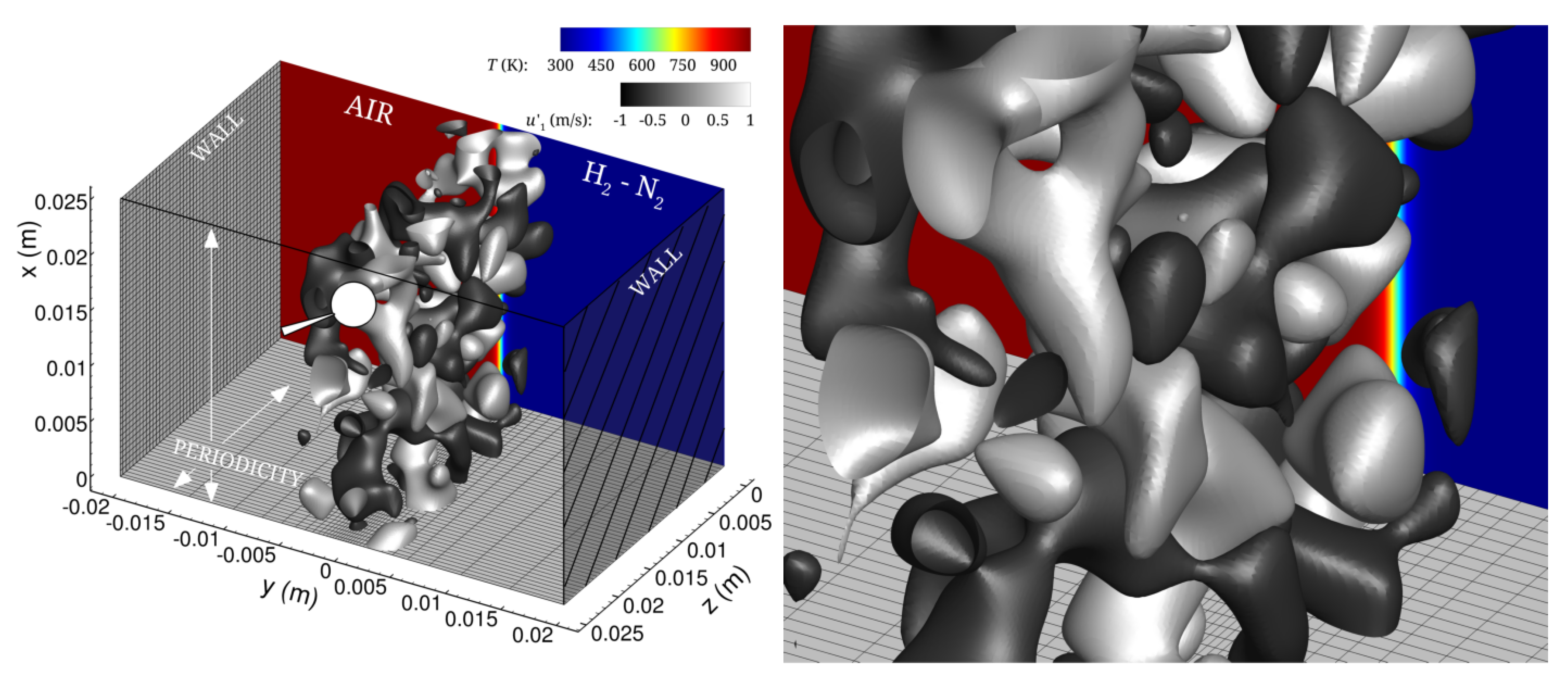
2.3. Problem Description

We consider an auto-ignition problem in a stationary mixing layer formed between a hydrogen/nitrogen mixture (0.1 H${}_2$/ 0.9 N${}_2$) at 300 K and hot air (1000 K). Figure 1 shows the computational domain ($L_x\times L_y\times L_z=0.025\times 0.04\times 0.025$ m${}^3$) in which in the vicinity of its centre ($y=0$) isotropic (HIT) or anisotropic (HAT) initial velocity fluctuations ($u^{\prime }$) are generated. The iso-surfaces presented in Figure 1 correspond to sample initial velocity fluctuations in the ‘x’ direction equal to $-0.5$ m/s (light grey) and $0.5$ m/s (dark grey). The flow is periodic in the ‘x’ and ‘z’ directions and the no-slip walls are assumed at $y=\pm L_y/2$. The fuel concentration is given by $C\left(y\right)=(tanh(2y/\delta )+1)/2$, where $\delta$ denotes the initial vorticity thickness assumed to be equal $0.5$ mm.

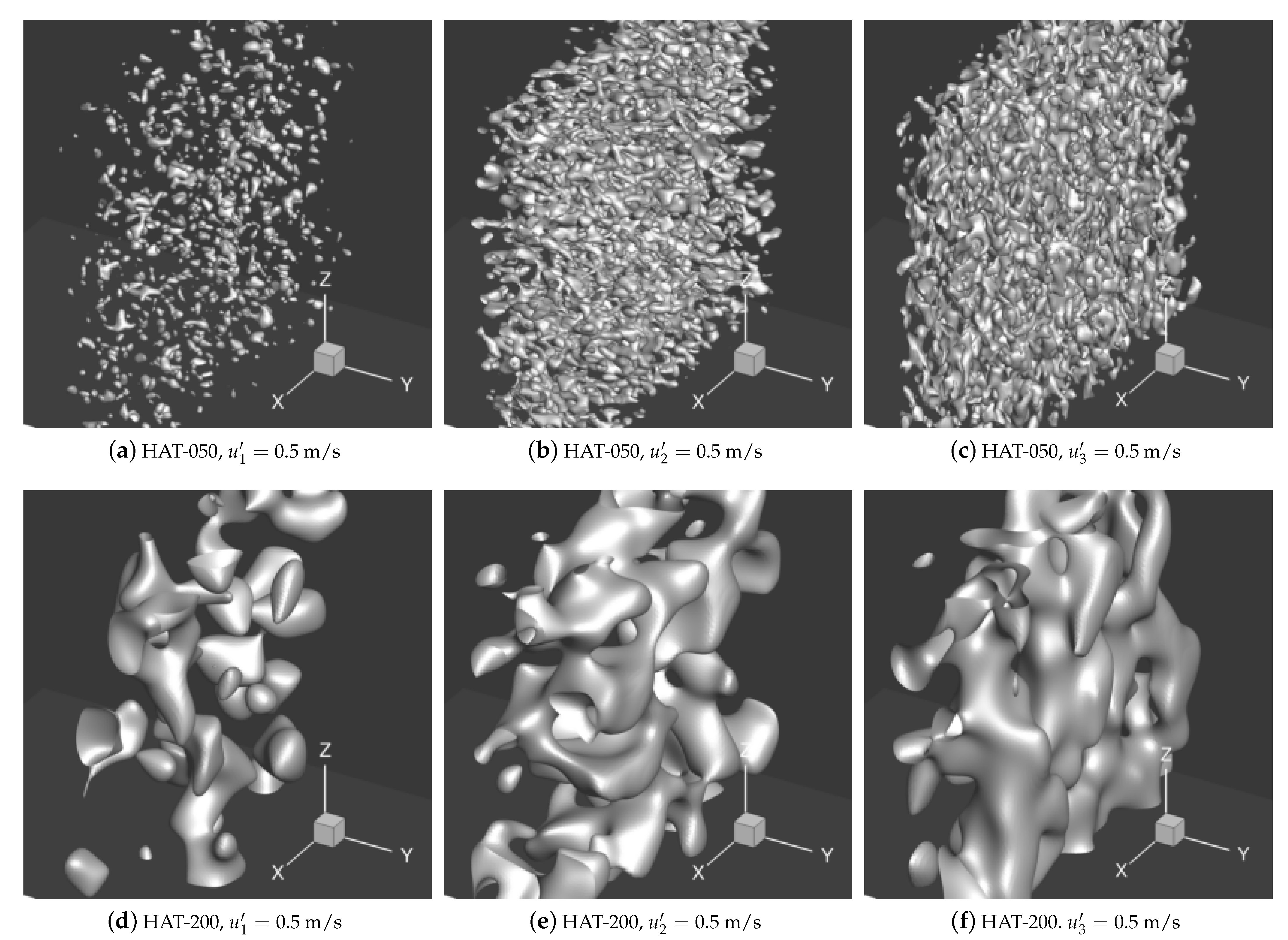
2.4. Initial Conditions

The turbulent velocity fields are generated by a method proposed by Orszag S. [44] that was originally used for the generation of the HIT fields. In the first step it relies on generation of an initial random velocity fluctuation ($u_{i,\mathrm{ran}}^{\prime }$) where the subscript ‘i’ stands for the ‘x’, ‘y’, ‘z’ direction. These random fields have the zero mean value and assumed RMS level. Then, they are transformed into the Fourier space where the particular velocity components are mutually correlated ($u_{i,\mathrm{ran}}^{\prime }\to u_i^{\prime }$) according to an assumed energy spectrum and requiring that $\nabla ·\mathbf{u}=0$. Due to these operations the RMS values of $u_{i,\mathrm{ran}}^{\prime }$ and $u_i^{\prime }$ are slightly different. In the present research we extend this procedure such that both HIT and HAT initial velocity fields could be generated. In the region of the mixing layer $\pm 10\delta$ the energy of the initial velocity is defined through the Passot–Pouquet kinetic energy spectrum defined as [45]:

$$E_i\left(k\right)=\frac{16}{3}\sqrt{\frac{2}{\pi }}{\displaystyle \frac{u_{i,\mathrm{RMS}}^2}{k_{i,0}}}{\left({\displaystyle \frac{k}{k_{i,0}}}\right)}^{4}exp\left[-2{\left({\displaystyle \frac{k}{k_{i,0}}}\right)}^2\right];E\left(k\right)=\sum _{i=1}^3{E}_i\left(k\right)$$

(7)

where k represents the wave number, $k_{i,0}$ is an adjustable wave number allowing generation of the velocity fluctuations with a required Taylor length scale ${\lambda }_i$ for a particular component of the velocity fluctuations. Their global RMS value is defined as $u_{\mathrm{RMS}}^{\prime }={\sum }_{i=1}^3{u}_{i,\mathrm{RMS}}^{\prime }/3$. In the HIT conditions the Taylor length scale is defined as $\lambda =\sqrt{\overline{u_{\mathrm{RMS}}^{\prime 2}}/\overline{{(\partial u_{\mathrm{RMS}}^{\prime }/\partial x)}^2}}$ where $u_{\mathrm{RMS}}^{\prime }$ is arbitrary velocity component and ‘x’—arbitrary direction. In the case of HAT the global Taylor length scale is defined, as $\lambda ={\sum }_{i=1}^3{\lambda }_i/3$ with ${\lambda }_i$ referring to particular directions. The initial HIT and HAT velocity fields are obtained by specifying either the same or different $u_{i,\mathrm{RMS}}^{\prime }$ and ${\lambda }_i$ in particular direction.

The turbulent Reynolds numbers can be computed either based on $u_{i,\mathrm{RMS}}^{\prime }$ and ${\lambda }_i$ as ${\mathrm{Re}}_{{\lambda }_i}=u_{i,\mathrm{RMS}}^{\prime }{\lambda }_i/\nu$, with $\nu$—the air kinematic viscosity, or based on the turbulent quantities that can be treated as representative for a given test case ($u_{\mathrm{RMS}}$, $\lambda$), i.e., ${\mathrm{Re}}_{\lambda }=u_{\mathrm{RMS}}^{\prime }\lambda /\nu$. In the present work we consider four HIT and four HAT cases with ${\mathrm{Re}}_{\lambda }\approx 50,100,150,200$ of which all parameters are given in

Table 1. Details of the simulations.

HIT
Case	$u_{1,\mathrm{RMS}}^{\prime }$ (m/s)	$u_{2,\mathrm{RMS}}^{\prime }$ (m/s)	$u_{3,\mathrm{RMS}}^{\prime }$ (m/s)	$u_{\mathrm{RMS}}^{\prime }$ (m/s)	$\lambda$ (m)				${\mathrm{Re}}_{\lambda }$				${\tau }_{\mathrm{t}}$ (s)
HIT-050	1.55	1.55	1.55	1.55	0.0005				50				0.0003
HIT-100	1.55	1.55	1.56	1.55	0.0010				99				0.0006
HIT-150	1.49	1.50	1.51	1.50	0.0016				156				0.0011
HIT-200	1.52	1.55	1.54	1.54	0.0020				199				0.0013
HAT
Case	$u_{1,\mathrm{RMS}}^{\prime }$ (m/s)	$u_{2,\mathrm{RMS}}^{\prime }$ (m/s)	$u_{3,\mathrm{RMS}}^{\prime }$ (m/s)	$u_{\mathrm{RMS}}^{\prime }$ (m/s)	${\lambda }_1$ (m)	${\lambda }_2$ (m)	${\lambda }_3$ (m)	$\lambda$ (m)	${\mathrm{Re}}_{{\lambda }_1}$	${\mathrm{Re}}_{{\lambda }_2}$	${\mathrm{Re}}_{{\lambda }_3}$	${\mathrm{Re}}_{\lambda }$	${\tau }_{\mathrm{t}}$ (s)
HAT-050	0.24	0.42	0.52	0.39	0.0017	0.0020	0.0021	0.0020	26	55	70	49	0.0050
HAT-100	0.33	0.59	0.73	0.55	0.0024	0.0029	0.0030	0.0028	51	108	140	97	0.0050
HAT-150	0.40	0.71	0.89	0.67	0.0030	0.0037	0.0038	0.0035	78	166	218	150	0.0053
HAT-200	0.47	0.84	1.03	0.78	0.0034	0.0041	0.0043	0.0039	101	221	283	196	0.0051

. Note, that due to above-mentioned procedure ($u_{i,\mathrm{ran}}^{\prime }\to u_i^{\prime }$) the final values of ${\mathrm{Re}}_{\lambda }$ slightly diverge from the assumed one. The last column shows the turbulent time scale defined as ${\tau }_{\mathrm{t}}=\lambda /u_{\mathrm{RMS}}^{\prime }$ to which we will refer discussing the impact of ${\tau }_{\mathrm{t}}/{\tau }_{\mathrm{ign},\mathrm{l}}$ on the ignition process. For HAT cases ${\tau }_{\mathrm{t}}$ remains on an almost constant level regardless of ${\mathrm{Re}}_{\lambda }$, whereas, in the HIT conditions its values pronouncedly depend on ${\mathrm{Re}}_{\lambda }$.

Differences between the isotropic and anisotropic initial turbulent field are shown in Figure 2 and Figure 3 presenting the iso-surfaces of $u_1^{\prime }=u_2^{\prime }=u_3^{\prime }=0.5$ m/s for the cases HIT-200 and HAT-050, HAT-200. It can be seen that in HIT-200 the spatial distributions of all velocity components are very similar and the iso-surfaces characterize the same size of the waviness. The situation in HAT is different as in this case the velocity fluctuations in the particular directions are associated with the corresponding ${\lambda }_i$ values. This causes significant modifications of their distributions and different wrinkling of the iso-surfaces. Moreover, it can be seen that the impact of ${\mathrm{Re}}_{\lambda }$ on the initial solution is large. In the case HAT-050 where ${\lambda }_i$ are small the size of the turbulent structure is also small compared to the case HAT-200. As will be shown later these differences have a significant influence on flame development. At this point, one should mention that in all HIT and HAT cases the length scales ${\lambda }_i$ are approximately ten times smaller than the sizes of the computational domain. Hence, the impact of the boundary conditions (walls, periodicity) on the evolving flow structures is very small and does not affect the ignition phenomenon.

2.5. Computational Details

All the computations have been performed on the mesh consisting of $192\times 128\times 192$. In Figure 1 every four mesh line is shown. The mesh nodes are distributed uniformly in the periodic directions ($\Delta x=\Delta z=1.31\times {10}^{-4}$ m) and are compacted in the ‘y’ direction. The minimum cell size is equal to $\Delta y_{\min }=5.59\times {10}^{-5}$ m and its average value in the region $-10\delta \le y\le +10\delta$ is $\Delta y_{-10\delta ,+10\delta }=1.11\times {10}^{-4}$ m. The simulations were conducted with a constant time step $\Delta t=1\times {10}^{-6}$ s corresponding to the CFL number approximately equal to 0.5, and lasted for the time period allowing the flame development across the whole domain.

When the simulations start the flow evolves and the initially imposed turbulent structures combine and develop. In LES, they are accurately represented on the numerical mesh provided that the Pope’s criterion is fulfilled [46], i.e., the ratio of the sub-grid ($k^{SGS}$) to the total kinetic energy ($k^{TOT}$) should be less than 0.2. The former is computed as $k^{SGS}={\mu }_t^2/{(\rho C\Delta )}^2$ ($C=0.1$ [47]). Figure 4 shows the contours of $k^{SGS}/k^{TOT}$ at the time instances before and during the ignition phase ($t\approx 1.0$ ms). It can be seen that the values of $k^{SGS}/k^{TOT}$ are very small and there are only a few places where they reach the level of 0.1. Additionally, in this figure we show the isolines of the ratio of the sub-grid to the molecular viscosity (${\mu }_t/\mu$). The values of ${\mu }_t$ are approximately two orders of magnitude smaller than $\mu$. All this means that the impact of the modeled sub-grid scale on the solution is very small and the computational mesh is appropriate for the present problem. Nevertheless, to show the level of dependence of the results on the mesh density, we performed the test computations on the mesh consisting of 70% more nodes, i.e., $224\times 160\times 224$ nodes.

3. Results

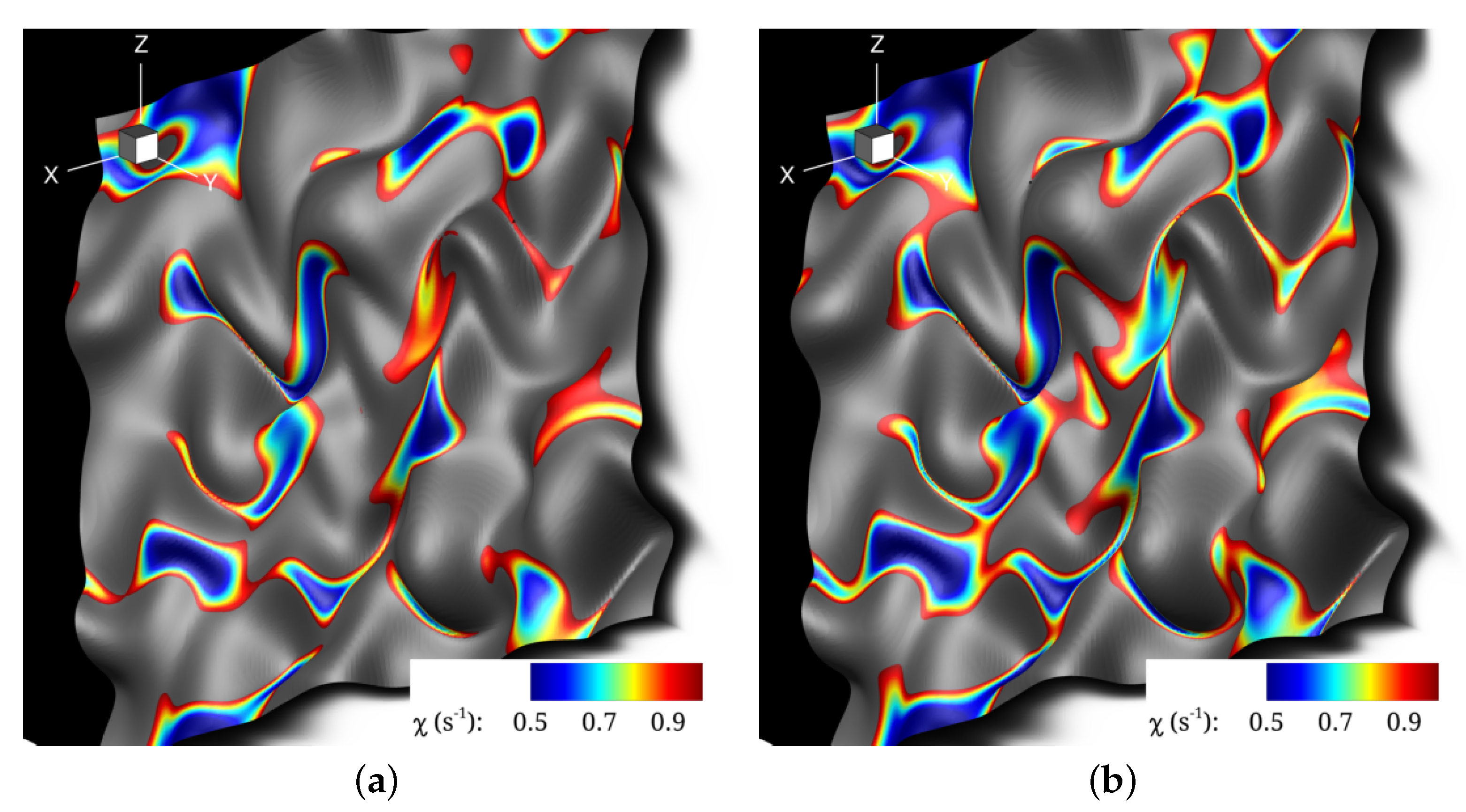
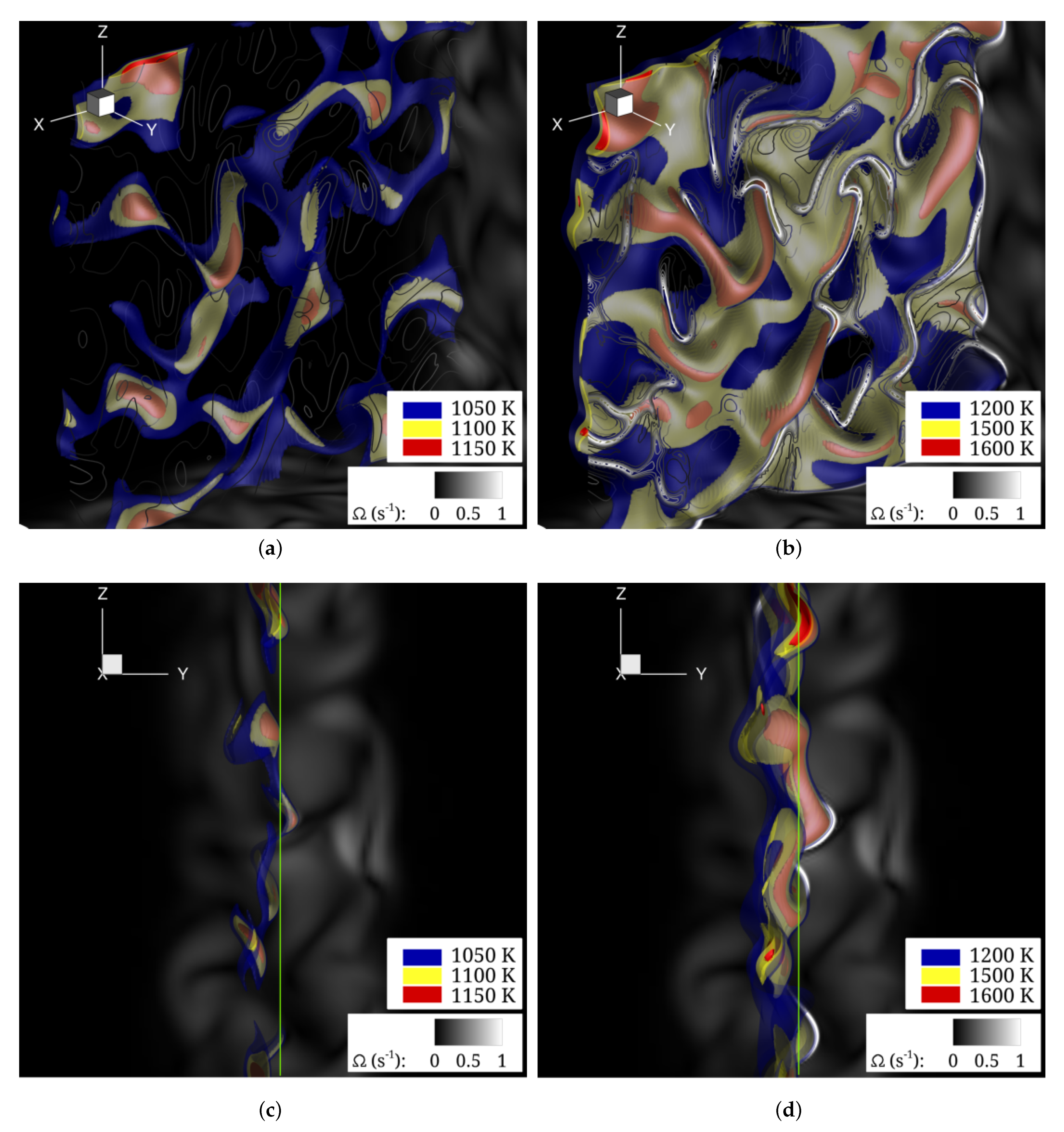
3.1. Auto-Ignition Scenario and Initial Flame Development Phase

After the simulation starts the fuel mixes with the hot air. The strength of the mixing process depends on the initial flow field but in all analyzed cases it leads to the conditions favorable for the auto-ignition, which is discussed below for the case HAT-200. In agreement with the findings of Mastorakos et al. [18] the ignition spots have the highest probability to appear in the places with the mixture composition corresponding to the most reactive mixture fraction (${\xi }_{\mathrm{MR}}=0.0178$) and where the scalar dissipation rate is low. In this work the mixture fraction $\xi$ is computed following the Bilger’s definition:

$$\xi =\frac{(Y_{\mathrm{H}}-Y_{\mathrm{H},\mathrm{o}})/2W_{\mathrm{H}}-(Y_{\mathrm{O}}-Y_{\mathrm{O},\mathrm{o}})/W_{\mathrm{O}}}{(Y_{\mathrm{H},\mathrm{f}}-Y_{\mathrm{H},\mathrm{o}})/2W_{\mathrm{H}}-(Y_{\mathrm{O},\mathrm{f}}-Y_{\mathrm{O},\mathrm{o}})/W_{\mathrm{O}}}$$

(8)

where Y’s are the elemental mass fractions, W’s are the atomic weights and the subscripts, $\mathrm{f}$ and $\mathrm{o}$, correspond to the fuel and air, $\mathrm{H}$ and $\mathrm{O}$ refer to the hydrogen and oxygen atoms, respectively. The scalar dissipation rate is defined as $\chi =2D\frac{\partial \xi }{\partial x_i}\frac{\partial \xi }{\partial x_i}$. Figure 5 shows the iso-surface of the most reactive mixture fraction coloured by the scalar dissipation rate at the time moments $t=0.9$ ms and $t=1.0$ ms from the beginning of the simulation. It can be seen that there are preferred locations (small $\chi$) in which the ignition spots can appear. Comparing the presented solutions, one can notice that during $0.1$ ms the flow evolves only slightly, however, in this time the flame kernels significantly grow and propagate towards the stoichiometric mixture (${\xi }_{\mathrm{ST}}=0.225$). At the later time the flame develops along ${\xi }_{\mathrm{ST}}$ and eventually expands across the mixing layer. Figure 6 shows semi-transparent iso-surfaces of three different temperature values and the vorticity module ($\Omega$) contours in the time moments corresponding to the results presented in Figure 5. The high temperature regions seem to be distributed randomly, however, their localisations correlate well with low values of $\chi$ (Cf. Figure 5). It can be seen that between $t=0.9$ ms and $t=1.0$ ms the initially local flames have connected and spread almost along the entire ‘x-z’ cross-section of the computational domain.

The view along the ‘x’ direction (Figure 6c,d) shows that the regions of high temperature induce large local velocity gradients that manifest by a significant growth of the vorticity module (white contours). Its contours in the ‘x–z’ cross-section plane indicated by the green vertical line are shown in Figure 7. The presented results correspond to the time moments $t=0.6$ ms, $t=0.9$ ms and $t=1.0$ ms. It can be seen that before the auto-ignition occurs (Figure 7a) and during its initial phase (Figure 7b) the vorticity values are comparable and low, in general. However, at the later time (Figure 7c) the thermal expansion caused by an increasing flame volume accelerates the flow in the layers attached to it. In effect, in a direct flame vicinity the vorticity grows significantly. The contours of its high values ($\Omega \approx 1.0$) correspond to the places in which the analyzed cross-section plane crosses the high temperature iso-surface.

3.2. Analysis of the Flame Volume and Maximum Temperature Growth

The above-depicted auto-ignition process is qualitatively the same in all cases considered. In this section, we analyze how the differences in the initial solutions affect the moment of auto-ignition and the subsequent evolution of the flame kernel. As the reference solution we assume the auto-ignition process in the laminar conditions in which the velocity fluctuations are equal to zero and the mixing between the fuel and air is driven by the diffusion mechanism. The auto-ignition time corresponds to the moment when the maximum temperature in the domain reaches the level of 1% above the oxidizer temperature that is commonly used criterion [25,48]. In the reference laminar case it is equal to ${\tau }_{\mathrm{ign},\mathrm{l}}=0.86$ ms.

Figure 8 shows the temporal evolutions of the mass fraction of HO${}_2$, the maximum temperature in the computational domain and the flame volume $V_{\mathrm{f}}$ for the cases HAT-200 and HIT-200 as the function of a normalised time $\tau =t/{\tau }_{\mathrm{ign},\mathrm{l}}$. The radical HO${}_2$ is the so-called preignition species whose appearance precedes the auto-ignition process and the temperature rise. The flame volume is a measure of the flame growth at its later phase. This parameter is defined as the sum of the volume of the computational cells in which the temperature is larger than 1200 K, i.e., $V_{\mathrm{f}}=\sum V_{\mathrm{cell}}^{T>1200K}$. The results presented in Figure 8 were obtained applying 4 and 8 stochastic fields ($N_s$ in Equation (5)). It can be seen that their number has only a minor influence on the solutions. The existing differences are very low and only quantitative, which confirms that the applied combustion model provides the results that can be regarded as independent of $N_s$. Regarding the temporal evolution of HO${}_2$ shown in Figure 8a one can see that the turbulence speeds up the preignition phase. A sudden rise of HO${}_2$ around $\tau =1.0$ is related to the auto-ignition phenomenon accompanied by a steep growth of the maximum temperature ($T_{\max }$) presented in Figure 8b. A close inspection on the ignition times shows that HIT-200 is characterized by a shorter ignition delay compared to HAT-200, though the differences are very small ($\approx 1\%{\tau }_{\mathrm{ign},\mathrm{l}}$). The exact values are $\tau =0.932$ for HIT-200 and $\tau =0.945$ for HAT-200 when 4 stochastic fields are applied. Apparently, the conditions favorable for the ignition occurs in both these cases with nearly the same probability. Much more pronounced are the differences in the maximum temperature at the later stage when the flame starts to grow and propagate. For instance, at $\tau =1.1$ it can be seen that in the case HIT-200 $T_{\max }$ is 230 K higher. However, when the flames are well established the difference in $T_{\max }$ vanishes and at $\tau =1.25$$T_{\max }$ in HIT-200 is only 40 K larger than in HAT-200.

The temporal evolution of $V_{\mathrm{f}}$ is presented in Figure 8c. It can be seen that $V_{\mathrm{f}}$ starts growing immediately after the temperature rise. Initially, its increase in HIT-200 and HAT-200 as well as for the laminar initial conditions is almost the same. Substantial differences are seen only when $T_{\max }$ values in all the cases become similar ($\tau \approx 1.25$). From this moment the flame expands significantly faster in the case HIT-200 and at the end of the simulation time its volume is approximately 20% larger than in HAT-200. This means that the significant differences in the initial flow conditions have a larger impact on the flame propagation phase than on its initialization and very early development.

Figure 9 shows the temporal evolution of the maximum temperature for all the cases from Table 1. The results corresponding to HIT and HAT are normalized such that the values $T_{\max }$ are divided by $T_{\max ,\mathrm{lam}}$ obtained for the laminar initial conditions at the end of the simulation time ($\tau =1.45$). It enables the comparison of the shapes of profiles and allows us to better quantify the impact of ${\mathrm{Re}}_{\lambda }$ and the initial regimes. It can be seen that the auto-ignition always occurs faster for the turbulent initial conditions. To some extent, this seems to contradict with the findings of [19] who observed that for ${\tau }_{\mathrm{t}}/{\tau }_{\mathrm{ign},\mathrm{l}}<1$ (the cases HIT-050, HIT-100, see ${\tau }_{\mathrm{t}}$ values in Table 1) the auto-ignition in turbulent flow was slightly retarded. There, however, the initial conditions characterized a strong turbulence that could have induced large values of the scalar dissipation rate delaying the ignition. Among the HIT cases $T_{\max }$ grows significantly faster during the entire simulation time when the Reynolds number is large (${\mathrm{Re}}_{\lambda }=150$ and ${\mathrm{Re}}_{\lambda }=200$). In the HAT conditions $T_{\max }$ is much less dependent on ${\mathrm{Re}}_{\lambda }$ and the turbulence level has a negligible impact on the ignition delay. This is because in the HAT cases, the turbulent time scale is nearly constant (${\tau }_{\mathrm{t}}/{\tau }_{\mathrm{ign},\mathrm{l}}=5.8-6.1$).

Figure 9 additionally shows the solutions obtained for the lowest Reynolds number on the 70% denser mesh. Analysis of these results aims to complement the discussion on the very low level of the sub-grid kinetic energy presented in Section 2.5. It confirms the accuracy of the performed simulations. It can be seen that the use of significantly more mesh points virtually does not affect the obtained profiles. The difference in predicting the auto-ignition time is less than $0.5\%{\tau }_{\mathrm{ign},\mathrm{l}}$, whereas the difference in respect to $T_{\max }$ during the flame development phase does not exceed 1% $T_{\max ,\mathrm{lam}}$. Taking into account that these results were obtained for the cases at ${\mathrm{Re}}_{\lambda }=50$ with very tiny initial flow structures it can be deduced that the basic mesh is appropriate also for the cases with larger vortices (${\mathrm{Re}}_{\lambda }=100,150,200$).

The normalised flame volume presented in Figure 10a ($V_{\mathrm{f}}/V_{\mathrm{f},\mathrm{lam}}$) is found to be analogously affected by the initial conditions. The differences between the particular solutions are substantial and grow with time. In the HIT conditions the mixing process turns out to be much more intense than in the HAT regimes. This enhances the flame propagation across the mixing layer, and in effect, at the end of simulations the flame volumes in the isotropic regimes are significantly larger. Even for the smallest ${\mathrm{Re}}_{\lambda }$ (HIT-050) $V_{\mathrm{f}}$ is larger than in any HAT case. In the case HIT-50 $V_{\mathrm{f}}$ is 25% larger than $V_{\mathrm{f},\mathrm{lam}}$, whereas in the case HAT-050 $V_{\mathrm{f}}$ and $V_{\mathrm{f},\mathrm{lam}}$ are comparable.

Figure 10b presents the instantaneous variation of the flame volume $d{V}_{\mathrm{f}}/d\tau$. It shows that the anisotropy causes a faster flame growth at an early stage of the flame kernel propagation ($\tau =1.04\text{–}1.1$) and the steepest change of the profile is found for the case HAT-050. In the later time ($\tau =1.12\text{–}1.22$) $d{V}_{\mathrm{f}}/d\tau$ is almost constant for all HAT cases that means that in this period of time the flame volumes grow in the time linearly. It can be seen that the values of $d{V}_{\mathrm{f}}/d\tau$ for HAT-100, HAT-150 and HAT-200 are practically the same and visibly larger than for HAT-050. This suggests that for the HAT conditions there is some threshold value of ${\mathrm{Re}}_{\lambda }$ (or ${\mathrm{Re}}_{{\lambda }_i}$) above which the flame growth is the fastest and only weakly dependent on ${\mathrm{Re}}_{\lambda }$. The situation is significantly different in the HIT regimes. The differences in $d{V}_{\mathrm{f}}/d\tau$ in particular cases are seen over the entire simulation time. Moreover, the profiles have a significantly different character with a well-marked maximum at $\tau \approx 1.25$. This corresponds to the time moment when the maximum temperatures in the domain for all HIT cases reach virtually the same level (see Figure 9a) and when the values of the flame volumes start to visibly diverge (see Figure 10a). The largest values of $d{V}_{\mathrm{f}}/d\tau$ are in the cases HIT-100 and HIT-150. Unlike as in the HAT conditions, this could suggest that when the initial turbulent field is isotropic there is an optimal moderate value of ${\mathrm{Re}}_{\lambda }$ at which the flame expansion is the most dynamic.

Figure 11 shows the contours of the mixture fraction $\xi$ and isolines of the selected values of the heat release in the central ‘y–x’ cross-section plane. The subfigures on the left half of Figure 11 correspond to the HIT conditions and on the right half to the HAT regimes. The presented results correspond to two time moments: (i) $\tau =1.1$ (upper row), when for the HAT cases $d{V}_{\mathrm{f}}/d\tau$ reaches the constant level; (ii) $\tau =1.23$ (bottom row), when for the HIT cases $d{V}_{\mathrm{f}}/d\tau$ are maximal. It can be seen that in the HIT conditions the distribution of the mixture fraction is much more wrinkled compared to the HAT regimes, especially in the cases HIT-050 and HIT-100. The heat release isolines are locally torn and the flame sources are dispersed. In effect, in these conditions the flame volume initially ($\tau =1.1\text{–}1.23$) grows slower than in the HAT regimes (Cf. Figure 10). The situation changes at the later time when the wrinkling translates to a larger surface area where the flame can appear (${\xi }_{\mathrm{MR}}$) and along which it can propagate. The increase of ${\mathrm{Re}}_{\lambda }$ in the HIT conditions smoothes the mixture fraction contours, i.e., the flow structures become larger and local small wrinkles vanish. In the HAT conditions the change of ${\mathrm{Re}}_{\lambda }$ causes the opposite behavior. In the case HAT-050 the values of ${\mathrm{Re}}_{{\lambda }_{1,2}}$ (‘x’ and ‘y’ direction) are small (see Table 1) and the mixing zone between the fuel and oxidiser is almost flat. The heat release isolines are continuous and extend over almost the entire ‘z–x’ plane. Unlike as in the HIT conditions, the increase of ${\mathrm{Re}}_{\lambda }$ makes the mixture fraction distribution more complex. This is the effect of mutual interactions between the flow scales along with the particular directions. The large initial value of $u_{3,\mathrm{RMS}}^{\prime }$ corresponding to ${\mathrm{Re}}_{{\lambda }_3}$ induces velocity fluctuations both in the ‘x’ and ‘y’ direction leading to pronounced wrinkling of the flame surface.

4. Conclusions

The large eddy simulation method combined with Eulerian Stochastic Fields was applied to study the auto-ignition mechanism in the stationary mixing layer with the initial isotropic (HIT) and anisotropic (HAT) velocity field. The dynamics of the turbulent flames was compared to the laminar case including the entire combustion process starting from the auto-ignition, through the propagation of the flame kernels, up to the time moment when the flame developed along with the mixing layer. The ignition delay was found to be shorter for all the turbulent cases and the minor impact of the initial Reynolds number (${\mathrm{Re}}_{\lambda }$) was observed only for the HIT regimes. Contrary to the ignition times, the evolution of the flame temperature, the flame size and its temporal growth were found to be significantly dependent on ${\mathrm{Re}}_{\lambda }$, both in the HIT and HAT conditions. For its higher values (${\mathrm{Re}}_{\lambda }>50$) the flame volumes turned out to be at least 25% larger than in the laminar conditions. At the same time, the differences between the flames in HIT and HAT conditions were observed at the level of 22–34%, with the larger impact of ${\mathrm{Re}}_{\lambda }$ in the HIT cases. It was found that the anisotropy of the initial velocity field seeds up the initial flame kernel growth but when the flame is developed it spreads over the domain slower than in the isotropic turbulent field. Analysis of the time evolution of flame volume variation has shown that in the HAT regimes its profiles characterize a plateau over some period of time, whereas in the HIT conditions distinct maxima occur. The flame surface waviness in the HIT regimes was found to be definitively more complex in the direction in which the velocity fluctuations and turbulent length scale were larger. It was observed that the increase of ${\mathrm{Re}}_{\lambda }$ in the HIT conditions smoothers the flame surface, whereas in the HAT cases it makes the flame surface more wavy.

The performed research showed that depending on the type of initial conditions the flame dynamics can be significantly different and can be more or less dependent on ${\mathrm{Re}}_{\lambda }$. In the HAT conditions the ${\mathrm{Re}}_{\lambda }$ values were set by changing the velocity fluctuations and turbulent length scales in each direction. In the future investigations, it would be advisable to consider the cases in which one of these parameters is kept constant while the other changes such to have the resulting ${\mathrm{Re}}_{\lambda }$ the same. Such an analysis would give separate information to what extent the flame evolution depends on the turbulence intensity/length scale in the particular directions (perpendicular or parallel to the flame surface).

References

1. Mastorakos, E. Ignition of turbulent non-premixed flames. Prog. Energy Combust. Sci. 2009, 35, 57–97. [Google Scholar] [CrossRef]
2. Mastorakos, E. Forced ignition of turbulent spray flames. Proc. Combust. Inst. 2017, 36, 2367–2383. [Google Scholar] [CrossRef] [Green Version]
3. Klimenko, A.; Bilger, R. Conditional moment closure for turbulent combustion. Prog. Energy Combust. Sci. 1999, 25, 595–687. [Google Scholar] [CrossRef]
4. Navarro-Martinez, S.; Kronenburg, A.; Di Mare, F. Conditional moment closure for large eddy simulations. Flow Turbul. Combust. 2005, 75, 245–274. [Google Scholar] [CrossRef]
5. Triantafyllidis, A.; Mastorakos, E. Implementation issues of the conditional moment closure model in large eddy simulations. Flow Turbul. Combust. 2010, 84, 481–512. [Google Scholar] [CrossRef]
6. Valiño, L. A field Monte Carlo formulation for calculating the probability density function of a single scalar in a turbulent flow. Flow, Turbul. Combust. 1998, 60, 157–172. [Google Scholar] [CrossRef]
7. Haworth, D. Progress in probability density function methods for turbulent reacting flows. Prog. Energy Combust. Sci. 2010, 36, 168–259. [Google Scholar] [CrossRef]
8. Jones, W.; Navarro-Martinez, S. Large eddy simulation of autoignition with a subgrid probability density function method. Combust. Flame 2007, 150, 170–187. [Google Scholar] [CrossRef]
9. Wang, Z.; Cai, Z.; Sun, M.; Wang, H.; Zhang, Y. Large Eddy Simulation of the flame stabilization process in a scramjet combustor with rearwall-expansion cavity. Int. J. Hydrogen Energy 2016, 41, 19278–19288. [Google Scholar] [CrossRef]
10. Liu, B.; An, J.; Qin, F.; Li, R.; He, G.Q.; Shi, L.; Zhang, D. Large eddy simulation of auto-ignition kernel development of transient methane jet in hot co-flow. Combust. Flame 2020, 215, 342–351. [Google Scholar] [CrossRef]
11. Zhong, L.; Liu, C. Numerical analysis of end-gas autoignition and pressure oscillation in a downsized SI engine using large eddy simulation. Energies 2019, 12, 3909. [Google Scholar] [CrossRef] [Green Version]
12. Zhou, L.; Zhang, X.; Zhong, L.; Yu, J. Effects of Flame Propagation Velocity and Turbulence Intensity on End-Gas Auto-Ignition in a Spark Ignition Gasoline Engine. Energies 2020, 13, 5039. [Google Scholar] [CrossRef]
13. Wang, Y.; Wei, H.; Zhou, L.; Zhang, X.; Zhong, L. Effects of reactivity inhomogeneities on knock combustion in a downsized spark-ignition engine. Fuel 2020, 278, 118317. [Google Scholar] [CrossRef]
14. Tyliszczak, A.; Cavaliere, D.E.; Mastorakos, E. LES/CMC of blow-off in a liquid fueled swirl burner. Flow Turbul. Combust. 2014, 92, 237–267. [Google Scholar] [CrossRef] [Green Version]
15. Schiavo, E.L.; Laera, D.; Riber, E.; Gicquel, L.; Poinsot, T. On the impact of fuel injection angle in Euler–Lagrange large eddy simulations of swirling spray flames exhibiting thermoacoustic instabilities. Combust. Flame 2021, 227, 359–370. [Google Scholar] [CrossRef]
16. Wang, Z.; Hu, B.; Fang, A.; Zhao, Q.; Chen, X. Analyzing lean blow-off limits of gas turbine combustors based on local and global Damköhler number of reaction zone. Aerosp. Sci. Technol. 2021, 111, 106532. [Google Scholar] [CrossRef]
17. Nassini, P.C.; Pampaloni, D.; Meloni, R.; Andreini, A. Lean blow-out prediction in an industrial gas turbine combustor through a LES-based CFD analysis. Combust. Flame 2021, 229, 111391. [Google Scholar] [CrossRef]
18. Mastorakos, E.; Baritaud, T.; Poinsot, T. Numerical simulations of autoignition in turbulent mixing flows. Combust. Flame 1997, 109, 198–223. [Google Scholar] [CrossRef]
19. Im, H.; Chen, J.; Law, C. Ignition of Hydrogen-Air Mixing Layer in Turbulent Flows. Symp. (Int.) Combust. 1998, 27, 1047–1056. [Google Scholar] [CrossRef] [Green Version]
20. Doom, J.; Mahesh, K. DNS of auto–ignition in turbulent diffusion H2/air flames. In Proceedings of the 47th AIAA Aerospace Sciences Meeting including The New Horizons Forum and Aerospace Exposition, Orlando, FL, USA, 5–8 January 2009; p. 240. [Google Scholar]
21. Chakraborty, N.; Mastorakos, E. Direct numerical simulations of localised forced ignition in turbulent mixing layers: The effects of mixture fraction and its gradient. Flow Turbul. Combust. 2008, 80, 155–186. [Google Scholar] [CrossRef]
22. Wawrzak, A.; Tyliszczak, A. A spark ignition scenario in a temporally evolving mixing layer. Combust. Flame 2019, 209, 353–356. [Google Scholar] [CrossRef]
23. Rosiak, A.; Tyliszczak, A. LES-CMC simulations of a turbulent hydrogen jet in oxy-combustion regimes. Int. J. Hydrogen Energy 2016, 41, 9705–9717. [Google Scholar] [CrossRef]
24. Markides, C.; Mastorakos, E. An experimental study of hydrogen autoignition in a turbulent co-flow of heated air. Proc. Combust. Inst. 2005, 30, 883–891. [Google Scholar] [CrossRef]
25. Stanković, I.; Triantafyllidis, A.; Mastorakos, E.; Lacor, C.; Merci, B. Simulation of hydrogen auto-ignition in a turbulent co-flow of heated air with LES and CMC approach. Flow, Turbul. Combust. 2011, 86, 689–710. [Google Scholar] [CrossRef] [Green Version]
26. Geurts, B. Elements of Direct and Large-eddy Simulation; R.T. Edwards: Philadelphia, PA, USA, 2004. [Google Scholar]
27. Vreman, A. An eddy-viscosity subgrid-scale model for turbulent shear flow: Algebraic theory and applications. Phys. Fluids 2004, 16, 3670–3681. [Google Scholar] [CrossRef]
28. Branley, N.; Jones, W. Large eddy simulation of a turbulent non-premixed flame. Combust. Flame 2001, 127, 1914–1934. [Google Scholar] [CrossRef]
29. Cook, A.W.; Riley, J.J. Direct numerical simulation of a turbulent reactive plume on a parallel computer. J. Comput. Phys. 1996, 129, 263–283. [Google Scholar] [CrossRef]
30. Tyliszczak, A. A high-order compact difference algorithm for half-staggered grids for laminar and turbulent incompressible flows. J. Comput. Phys. 2014, 276, 438–467. [Google Scholar] [CrossRef]
31. Tyliszczak, A. High-order compact difference algorithm on half-staggered meshes for low Mach number flows. Comput. Fluids 2016, 127, 131–145. [Google Scholar] [CrossRef]
32. Laizet, S.; Lamballais, E. High-order compact schemes for incompressible flows: A simple and efficient method with quasi-spectral accuracy. J. Comput. Phys. 2009, 228, 5989–6015. [Google Scholar] [CrossRef]
33. Brown, P.N.; Hindmarsh, A.C. Hindmarsh. Reduced Storage Matrix Methods in Stiff ODE Systems. J. Appl. Math. Comput. 1989, 31, 40–91. [Google Scholar] [CrossRef]
34. Shu, C.W. High-order finite difference and finite volume WENO schemes and discontinuous Galerkin methods for CFD. Int. J. Comput. Fluid Dyn. 2003, 17, 107–118. [Google Scholar] [CrossRef]
35. Kee, R.J.; Rupley, F.M.; Miller, J.A. CHEMKIN-II: A FORTRAN Chemical Kinetics Package for the Analysis of Gas-Phase Chemical Kinetics; SAND89-8009B, UC-706; Sandia National Laboratories: Albuquerque, NM, USA, 1993.
36. Bazooyar, B.; Darabkhani, H.G. Analysis of flame stabilization to a thermo-photovoltaic micro-combustor step in turbulent premixed hydrogen flame. Fuel 2019, 257, 115989. [Google Scholar] [CrossRef]
37. Mueller, M.; Kim, T.; Yetter, R.; Dryer, F. Flow reactor studies and kinetic modeling of the H2/O2 reaction. Int. J. Chem. Kinet. 1999, 31, 113–125. [Google Scholar] [CrossRef]
38. Boguslawski, A.; Wawrzak, K.; Tyliszczak, A. A new insight into understanding the Crow and Champagne preferred mode: A numerical study. J. Fluid Mech. 2019, 869, 385–416. [Google Scholar] [CrossRef]
39. Tyliszczak, A.; Geurts, B.J. Controlling spatio-temporal evolution of natural and excited square jets via inlet conditions. Int. J. Heat Fluid Flow 2019, 80, 108488. [Google Scholar] [CrossRef]
40. Tyliszczak, A. LES–CMC study of an excited hydrogen flame. Combust. Flame 2015, 162, 3864–3883. [Google Scholar] [CrossRef]
41. Kuban, Ł.; Stempka, J.; Tyliszczak, A. Numerical Analysis of the Combustion Dynamics of Passively Controlled Jets Issuing from Polygonal Nozzles. Energies 2021, 14, 554. [Google Scholar] [CrossRef]
42. Wawrzak, A.; Tyliszczak, A. Implicit LES study of spark parameters impact on ignition in a temporally evolving mixing layer between H2/N2 mixture and air. Int. J. Hydrogen Energy 2018, 43, 9815–9828. [Google Scholar] [CrossRef]
43. Wawrzak, A.; Tyliszczak, A. Study of a Flame Kernel Evolution in a Turbulent Mixing Layer Using LES with a Laminar Chemistry Model. Flow Turbul. Combust. 2020, 105, 807–835. [Google Scholar] [CrossRef]
44. Orszag, S.A. Numerical Methods for the Simulation of Turbulence. Phys. Fluids 1969, 12, 250–257. [Google Scholar] [CrossRef]
45. Passot, T.; Pouquet, A. Numerical simulation of compressible homogeneous flows in the turbulent regime. J. Fluid Mech. 1987, 181, 441–466. [Google Scholar] [CrossRef]
46. Pope, S. Ten questions concerning the large-eddy simulation of turbulent flows. New J. Phys. 2004, 6, 1–25. [Google Scholar] [CrossRef] [Green Version]
47. Pope, S. Turbulent Flows; IOP Publishing: Bristol, UK, 2001. [Google Scholar]
48. Jones, W.; Navarro-Martinez, S. Study of hydrogen auto-ignition in a turbulent air co-flow using a Large Eddy Simulation approach. Comput. Fluids 2008, 37, 802–808. [Google Scholar] [CrossRef]
Figure 1. Stationary mixing layer problem: the computational domain and mesh (grid lines are drawn every four at the side boundary); initial temperature (contours at the side boundary) and anisotropic turbulent field (iso-surfaces of u 1 ).
Energies 14 01869 g001
Figure 2. Iso-surfaces of the initial velocity fluctuations in the case homogeneous isotropic turbulence (HIT-200).
Energies 14 01869 g002
Figure 3. Iso-surfaces of the initial velocity fluctuations in the cases homogeneous anisotropic turbulence (HAT-050 and HAT-200).
Energies 14 01869 g003
Figure 4. Contours of k S G S / k T O T and the iso-lines of μ t / μ in the central ‘y–x’ cross-section plane. The results obtained for the case HAT-200 before (a,b) and during the ignition phase (c).
Energies 14 01869 g004
Figure 5. Iso-surface of the most reactive mixture fraction coloured by the scalar dissipation rate limited to χ = 1.0 s 1 (the grey regions correspond to χ > 1.0 s 1 ). The results obtained for the case HAT-200 in two time moments: (a) t = 0.9 ms; (b) t = 1.0 ms.
Energies 14 01869 g005
Figure 6. 3D temperature iso-surfaces and the vorticity contours. The results obtained for the case HAT-200 in two time moments: (a) t = 0.9 ms (3D view); (b) t = 1.0 ms (3D view); (c) t = 0.9 ms (‘y-z’ plane); (d) t = 1.0 ms (‘y-z’ plane).
Energies 14 01869 g006
Figure 7. Vorticity module contours for the case HAT-200 in the central ‘x-z’ cross-section plane at three different time instances corresponding to: (a) t = 0.6 ms—before the auto-ignition; (b) t = 0.9 ms—the first auto-ignition spots appear; (c) t = 1.0 ms—the flame expands along the ‘x-z’ directions and across the mixing layer in the ‘y’ direction.
Energies 14 01869 g007
Figure 8. Time evolution of: (a) maximum HO 2 concentration; (b) maximum temperature; (c) flame volume. Comparison of the solutions obtained in laminar and turbulent regimes using different number of stochastic fields.
Energies 14 01869 g008
Figure 9. Time evolution of the normalized maximum temperature in the conditions: (a) HIT; (b) HAT.
Energies 14 01869 g009
Figure 10. Time evolution of: (a) normalized flame volume; (b) variation of the flame volume.
Energies 14 01869 g010
Figure 11. Mixture fraction contours at the ‘y–x’ cross-section along with the iso-lines of heat release (red—2000 MJm 3 s 1 , black—5000 MJm 3 s 1 , blue—8000 MJm 3 s 1 ) at the time τ = 1.1 (a) HIT-050; (b) HIT-100; (c) HIT-200; (d) HAT-050; (e) HAT-100; (f) HAT-200 and τ = 1.23 (g) HIT-050; (h) HIT-100; (i) HIT-200; (j) HAT-050; (k) HAT-100; (l) HAT-200.
Energies 14 01869 g011