Article

Development and Validation of a Data-Driven Fault Detection and Diagnosis System for Chillers Using Machine Learning Algorithms

Department of Mechanical Engineering, Chonnam National University, Gwangju 61186, Korea
*
Author to whom correspondence should be addressed.
Energies 2021, 14(7), 1945; https://doi.org/10.3390/en14071945
Submission received: 10 February 2021 / Revised: 13 March 2021 / Accepted: 30 March 2021 / Published: 1 April 2021
(This article belongs to the Section F: Electrical Engineering)

Abstract

:
Fault detection and diagnosis (FDD) systems enable high cost savings and energy savings that could have economic and environmental impact. This study aims to develop and validate a data-driven FDD system for a chiller. The system uses historical operation data to capture quantitative correlations among system variables. This study evaluated the effectiveness and robustness of eight FDD classification methods based on the experimental data of the chiller (the ASHRAE 1043-RP project). The training data used for the FDD system is classified into four cases. Moreover, true and false positive rates are used to characterize the performance of the classification methods. The results show that local fault is not significantly sensitive to training data, and shows high classification accuracy for all cases. The system fault has a significant effect on the amount of data and the severity levels on the classification accuracy.

1. Introduction

Heating, ventilation, air conditioning, and refrigeration (HVAC&R) systems are widely used in commercial buildings. They consume a large amount of energy, which forms a major part of the total energy used in commercial buildings. However, poorly maintained, degraded, and improperly controlled equipment wastes 15–30% of the overall energy used in commercial buildings [1]. A chiller is the most important component in the HVAC&R system, which includes condensers, evaporators, refrigeration subsystems, and other parts [2]. Moreover, chillers operating under faulty conditions consume extra energy (up to 30% for commercial buildings) and incur a high cost, provide less comfort control, and generate bad indoor/outdoor air quality [3]. This can be solved by applying fault detection and diagnosis (FDD) systems, so that important faults can be detected and addressed promptly. The FDD method provides an effective means for ensuring efficient and reliable operation of HVAC&R systems [4].
Many researchers have applied FDD methods to detect and diagnose faults in chiller systems. In the ASHRAE project, Comstock and Braun [5] identified common chiller faults and built a database of chiller performance considering normal operations, severity levels, and operating conditions. The ASHRAE project became an active part of the FDD research, sponsoring several research projects. Wang and Cui [6] presented a combined qualitative model with a statistical approach and a principal component analysis (PCA) for a centrifugal chiller. The PCA-based method used sensor faults data for FDD to capture correlations among the measured variables. Han et al. [3,7] developed a statistical FDD method for the centrifugal chiller with a fixed-speed compressor and a thermal expansive valve (TXV). A hybrid support vector machine (SVM) was also developed based on the genetic algorithm (GA). It uses a GA until the accuracy reaches the desired limit or the best results can be found. Zhao [8] introduced the support vector data description (SVDD) algorithm, which finds the smallest volume of hypersphere in a high-dimensional feature space and classifies faults based on the boundary for classification. Hu [9] compared the conventional PCA with self-adaptive principal component analysis (APCA), which removes outliers for temperature sensor faults with an absolute value of less than 1 degree. Yan [10] combined an extended Kalman filter with a recursive SVM for the problem of the traditional FDD method, which requires a large amount of fault data. Fan et al. [11] introduced the three different SVM methods, and derived the accuracy rate of chiller FDD according to the number of features. Han et al. [12] developed least square (LS) SVM method, and compared LS-SVM to the accuracy of SVM and probabilistic neural networks (PNN) methods.
The data-driven FDD method uses historical operation data to capture quantitative correlations among system variables. With the development of sensor and computer technologies, real-time measurements provide space for data-driven FDD methods. Previous studies [3,4,5,6,7,8,9,10,11,12] have focused on the development of the FDD method, which exhibits high accuracy and performance. However, the methods have limitations, and the limitations are given below:
  • Complex process: Many researchers combine FDD methods and use data collected by the system and specific components. Analyzing and building such models consumes a lot of time and incurs high costs. For example, the residual method through PCA is suitable for chiller sensors but unsuitable for each component. The FDD model through PCA should determine the appropriate mathematical model for the data to distinguish normal data from fault data.
  • Excessive data usage: A large data set exhibits efficient performance in FDD, but the data are difficult to obtain because the data can only be obtained when an actual fault occurs. The performance is sensitive not only to the amount of data, but also the composition of the data. Therefore, it is better to carefully select the necessary severity and type of data. However, several methods overuse fault data without determining the exact severity level and type required.
This study finds the accuracy of detecting all kinds of faults and severity levels, which are the results of machine learning using limited data. Six well-known classification methods which were generated in the ASHRAE Project 1043-RP are applied to our FDD strategy: (1) refrigerant overcharge (RO), (2) refrigerant leakage (RL), (3) reduced evaporator water flow (FWE), (4) reduced condenser water flow (FWC), (5) non-condensable in refrigerant (NC), and (6) condenser fouling (CF) [5]. The proposed strategy uses the classification methods that use default hyperparameters to recognize the characteristics of training data and each classification method. We used the following models in this study: (1) logistic regression (LR), (2) SVM with three kernels, (3) random forest (RF), and (4) extreme gradient boosting (XGB). The classification methods used functions in the sklearn and XGB library [13,14]. Then, we have applied the grid search technique to our FDD strategy and found the hyperparameters. After that, we analyzed the cross-validation accuracy, and constructed a confusion matrix with test data and fault prediction data. We derived the true positive rate (TPR) value and false positive rate (FPR) from confusion matrix to verify the prediction accuracy for each method. Previous studies did not make a difference between training data and test data for severity levels, and used models that were trained with sufficient training data. However, in industrial sites and experiments, the majority of fault data have low severity levels, and it is difficult to obtain high severity fault data. This is also a limitation because faulty equipment is required to obtain fault data. Therefore, the proposed strategy in this study finds an optimal model by classifying the case into four categories for severity level and amount of data. This strategy has the advantage of easily verifying the performance of each classification method against a limited amount of data and severity levels.

2. Methodology

This study presents a data-driven FDD approach that uses machine learning classification methods to detect and diagnose depending on the amount of data and severity levels. Different fault types are discriminated based on normal and fault data. The structure of the proposed FDD method is illustrated in Figure 1. There are two processes which includes model training and test.
In the model training process, the training data set was classified into four cases. The classification criteria are the size of the training data set and the severity level of fault data. For Cases 1 and 2, the training data set is 30% of the total data set, and it represents a simulation with the “insufficient data set”. Among the insufficient data sets, Case 1 used two severity levels (LV1 and LV2), indicating that the amount of data and the severity levels of fault data were insufficient. For Case 2, four severity levels (LV1, LV2, LV3, and LV4) were used to train data, which indicates an insufficient amount of data. For Cases 3 and 4, 70% of the total data were used for the training data set, and it represents “sufficient data set”. For Case 3, the two severity levels were used in the training data set, and Case 3 indicates that the severity level of fault was insufficient. Case 4 is the situation when the amount of data and severity levels are sufficient.
After the classification of the cases, the training data go through a preprocessing process. The data preprocessing improves the quality of the input database. The data preprocessing process is divided into sub-processes: (1) data normalization and (2) feature selection. Data normalization includes feature transformations in a common range so that larger numeric feature values do not dominate the smaller numeric feature values. The StandardScaler of the sklearn library was used for data normalization. The standardScaler standardizes a feature by subtracting the mean and scaling to unit variance.
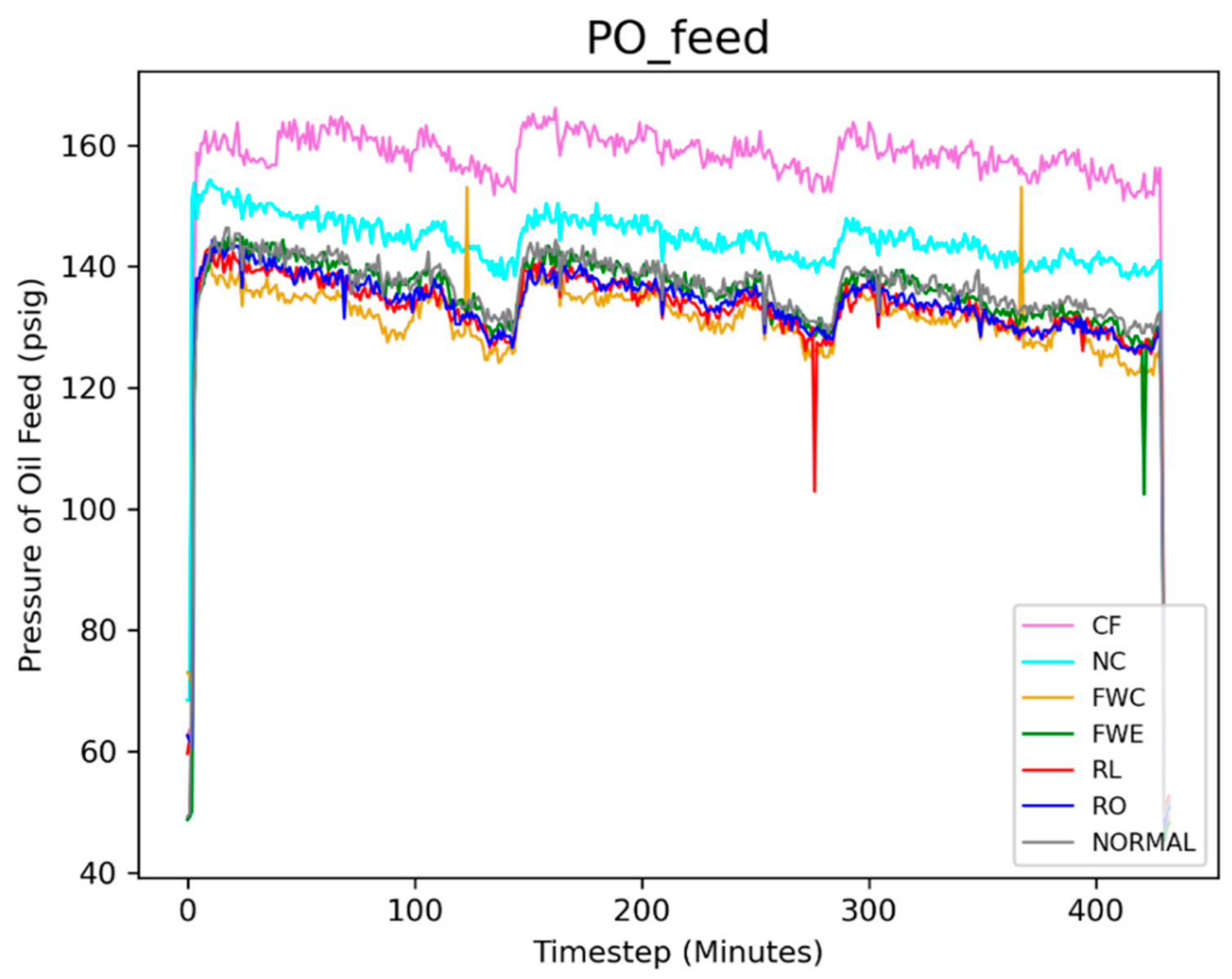
Feature selection helps improve model performance and predict all fault types because the feature characteristics are different for each fault. We select eight features, namely temperature of evaporator outlet (TEO), temperature of condenser outlet (TCO), flow water rate of cold (FWC), temperature of refrigerant condenser (TRC), temperature of refrigerant discharge (TR_dis), pressure of oil feed (PO_feed), valve position of evaporator (VE), and temperature of water in (TWI), which have been handled in the previous studies [15,16]. Figure 2 shows the example of the trends of the PO_feed for each fault and normal data. For CF and NC faults, the pressure values are higher than normal pressure, and the difference between CF and NC is clearly distinguished.
After data preprocessing, the training data pass through tuning hyperparameters to fit into each model. Each classification method has several tuning parameters. Choosing an appropriate tuning parameter is an important step to ensure good predictive performance. Tuning parameters are selected with the k-fold cross-validation (CV) technique [17,18]. It divides the training data set into approximately same-size k-folds. The first fold is used as a validation set, and the remaining folds are used to fit the model. The fitted model is predicted based on the validation set, and the accuracy of the model is measured using the validation set. This process is repeated for all the k-folds, and the CV accuracy score is obtained from the average accuracy of all k-folds. The k-fold CV accuracy can estimate the test accuracy before test data.
We used a grid search technique to find the optimal hyperparameter variable for each classification method and calculated the 10-fold CV accuracy for each grid hyperparameter variable. The grid search technique can find optimal hyperparameters by trying all the possible combinations of user-specified hyperparameters. Then, we performed a 10-fold CV technique for all the combinations to select optimal hyperparameters, for which the 10-fold CV accuracy was the highest. After the optimal hyperparameters were found, the model was refitted to generate the final classification method.
In the model test process, the test data set for all cases is the same. The test data set used 30% of the preprocessed data in the training data set and was classified into three methods. First, the classification method used the default hyperparameters specified by sklearn. The test results can be defined as a two-dimensional confusion matrix to evaluate the performance of the classification method in detecting and diagnosing normal and faulty operations [19]. The two-dimensional confusion matrix compares the actual and predicted classifications. Each element of the matrix represents the number of test observations and is used as TPR or FPR to evaluate the overall test accuracy rate. The confusion matrix consists of four components, and Table 1 lists the composition of the confusion matrix used in this study (for example, FWC), where TP (true positive) denotes the number of the cases for which the predicted class FWC fault and actual class coincided, TN (true negative) denotes the number of the cases for which the predicted class did not predict an FWC fault and the actual class was not an FWC fault, FP (false positive) denotes the number of the cases for which predicted class predicted an FWC fault and the actual class was not an FWC fault, and FN (false negative) denotes the number of the cases for which predicted class did not predict an FWC fault and the actual class happened to be an FWC fault. These four components help calculate TPR and FPR as follows:

2.1. Support Vector Machine

SVM has become an area of intense interest and research owing to its advantages in solving complex problems, which are characterized by nonlinear, high-dimensional, local minima, and small samples [3]. SVM is a classification method that aims to separate two data sets at maximum distance and is defined as (1) [20]:
f X = sgn w T K x , x + b
where sgn w T K x ,   x + b is the sign function, w and b represent the weight and the bias of the hyperplane, respectively, X is the training data, and x and x are input vector for SVM. Moreover, SVM classification method is trying to maximize a margin by minimizing weight. The minimize function is using a control tradeoff as shown in (2) [21]:
min 1 2 w T w + C i n ζ i
where C is the control tradeoff between smooth decision boundary and classifying training points correctly, and ζ i is a distance from decision boundary. SVM is a kernel-based classification method, and frequently used kernels include Linear, RBF, and Poly. The kernel-based classification method helps classify data easily by making higher-dimensional using kernels; each kernel is shown in the following Equation (3) [20]:
K x , x = x x , k e r n e l = L i n e a r exp γ x x 2 ,   k e r n e l = R B F γ x x + θ d ,   k e r n e l = P o l y
where γ is specified by hyperparameter gamma in RBF and Poly, d denotes the degree of polynomial function, and θ is the parameter to ensure high performance for nonlinear data in Poly. For the RBF and Poly classification methods, the hyperparameters are C and γ , but the default value for γ is 1 / { n feature × var X in default methods, where n feature is the number of features and var X is the variance of training data X . In this study, we uses three classification methods (Linear, RBF, and Poly) for SVM.

2.2. Logistic Regression

LR can be performed when dependent variables are bifurcated for predictive evaluation. LR is used to quantitatively describe the relationship between one dependent binary variable and one or more numeric nominal variables. LR estimates the data classification probability along the direction that minimizes the difference between the predicted and actual values. Probability analysis based on Equation (4) determines whether the data are normal or faulty [22,23,24,25].
p ^ = σ X = 1 1 + exp X
where σ X is the sigmoid logistic function whose output is in the range of zero to one, X is the training data, and p ^ is the output data; if p ^ > 0.5 , the data are detected as faulty, and if p ^ 0.5 , the data are detected as normal data.

2.3. Random Forest

RF integrates a large number of classification and regression trees (CART) [26]. RF has a better learning capacity than conventional machine learning techniques, such as SVM, RBF, and LR [27]. RF helps alleviate the overfitting problem owing to the sparseness of data in the sample space [28]. Compared to the multivariate linear regression method, higher accuracy was observed for models developed using the RF model when experimental data of a chiller were measured at short intervals [29]. The schematic of RF is shown in Figure 3. During the data training process, trees are randomly created, and the tree with the highest accuracy for sample data input is selected. The biggest feature of RF is that the trees have slightly different characteristics owing to their randomness, which improves the generalization performance.

2.4. Extreme Gradient Boosting

Gradient boosting algorithm (GBM) reduces loss with object function by combining sequential weak learners in a way that reduces residual of training data. XGB adds a regularization term to the GBM method and is a scalable machine learning system for CART [30]. The XGB method is as follows (5) [14]:
Y ^ = k = 1 m f k X , f k F
where Y ^ is the prediction value, X is the training data, and f k is a regularization function in the functional space F . The XGB method generates a loss function through the difference between the predicted and actual values and the regularization function. The loss function is as follows Equation (6) [14]:
loss   function = i n l Y ^ , Y + k = 1 m f k X
where l Y ^ , Y is the differentiable convex loss function, and Y is the target value. k m f k X is a regularization term. The regularization term prevents overfitting by giving penalizing loss as tree complexity increases.

3. System Description

The chiller data were generated in the ASHRAE Project 1043-RP [5]. The ASHRAE chiller fault data were used to train and test ensemble members and the integrated model where the experimental data represented a fault simulation for a 90 ton (approximately 316 kW) centrifugal chiller. The experiments simulated six typical faults and normal operation under 27 operation states; 64 parameters were obtained, including temperature, pressure, flow rate, valve position, electricity power, and cooling capacity. Among these, 40 were directly obtained from sensors, and 16 were calculated timely. The faults chosen for experimental simulation could be detected and diagnosed by monitoring the chiller. Based on the results of the chiller fault survey of ASHRAE 1043-RP, six typical faults were investigated in this study, which account for a major portion of the service calls, and each typical fault was monitored based on four severity levels (Table 2) [31]. RO, RL, FWE, and FCW faults have the same severity levels (10%, 20%, 30%, and 40%, respectively). The severity levels of NC are 1%, 2%, 3%, and 5%, and CF are 12%, 20%, 30%, and 45%, respectively. RO and RL faults were emulated by reducing or increasing the refrigerant charge depending on the severity levels. NC fault was emulated by adding 1% to 5% nitrogen to the refrigerant. FWE and FWC faults were emulated directly by reducing water flow rate in the condenser and evaporator by 10% to 40%. CF fault was emulated by plugging tubes into condenser [32].
The input and output of the datasets are shown in Table 3 below. The input data and output data are defined by the x value and y value of each classification model. The input data used the above-mentioned features, and the output data was classified as the fault types (RO, RL, NC, FWE, FWC, CF, and NORMAL) rather than the Boolean data type to detect and diagnostic the chiller faults.
As mentioned in Section 2, the proposed strategy is classified into four cases. Table 4 shows the number of training and test data set. We assume that the test data for all cases are the same. We randomly divided the total 11,691 fault data into two parts, a training data set containing 70% of the data (8183 fault data), and a test data set containing the remaining 3508 fault data. The randomly divided test data is used in all cases. The training data sets in Case 1 and 2 are 1948 and 3507 respectively. For Case 1 and Case 2, the number of training data set is lower than the number of test data set. In contrast, the training data sets in Case 3 and 4 are 4546 and 8183 respectively, and is over than the number of test data set.

4. Results

To explore the performance under various conditions of data and severity levels, we applied each classification method to four simulation cases. We implemented the following FDD strategies and compared their results:
  • Approach 1. First, we apply each classification method, which uses default parameters for the chiller data of the ASHRAE 1043-RP Project, compare the 10-fold CV accuracy for each default classification method.
  • Approach 2. Second, we apply each classification method, which uses the tuning parameters for the chiller data and compare the 10-fold CV accuracy of each classification method. The test results are discussed based on the confusion matrix, TPR, and FPR.
  • Approach 3. Finally, we determine the best classification method for each case based on the results generated by approach 1 and 2.
The proposed FDD strategy is tested with the data collected from the ASHRAE 1043-RP Project. All the classification methods were implemented using Python, especially sklearn and XGB library.

4.1. Case 1

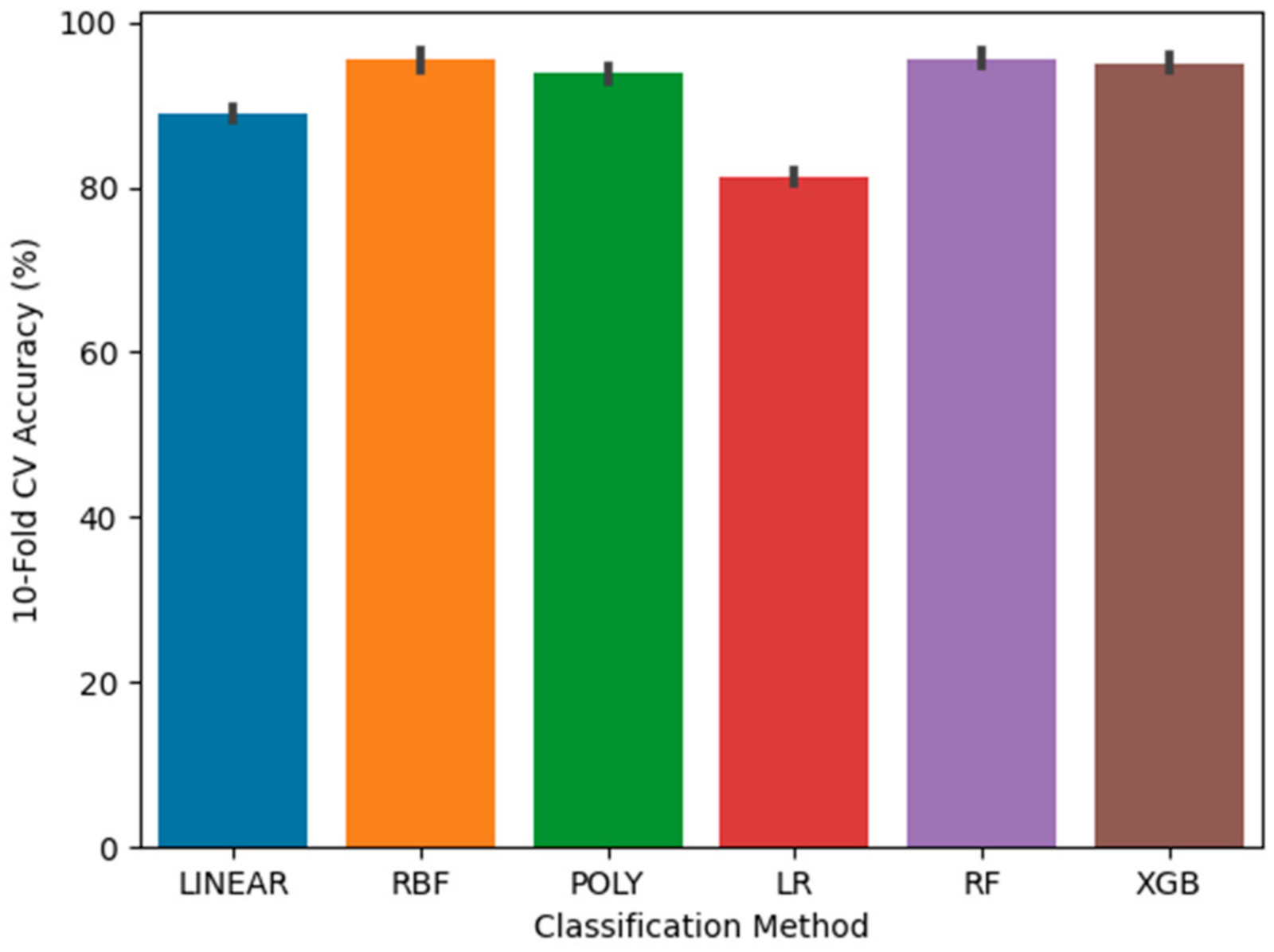
The training data set in Case 1 includes insufficient data with severity levels 1 and 2, and the test data are based on all the severity levels (1, 2, 3 and 4). The point of Case 1 is to find the optimal model to determine all the severity levels with the insufficient data and severity levels 1 and 2. As mentioned above, we derive a 10-fold CV accuracy value for each classification method. The 10-fold CV accuracy provides the reliability of the training data set and test results. Figure 4 shows the 10-fold CV accuracy for six classification methods. Each bar graph represents the average of 10-fold CV accuracy, and the black line represents the accuracy range. RF and XGB are the best classification methods, with average accuracy rates of 95.02% and 94.92%, respectively, and Poly is the weakest classification method, with an average accuracy rate of 73.97%. For Linear, RBF, and LR, the average accuracy rates are 87.99%, 81.06%, and 81.31%, respectively. A general XGB parameter uses “gbtree” as booster. RF and XGB, which involve using “tree” techniques, exhibited the highest training performance.
As mentioned in approach 2, hyperparameter tuning was performed for each classification method. Figure 5 shows the 10-fold CV accuracy of the parameter-tuned classification methods pertaining to Case 1. For RBF, Poly, RF, and XGB methods, the 10-fold CV accuracy is >90%, and for Linear and LR, the accuracy is <90%. RBF and RF are the best classification methods, with average accuracy rates of 95.43% and 95.64%, respectively, and Linear and LR are the weakest classification methods, with average accuracy rates of 89.01% and 81.36%, respectively. Poly and XGB have accuracy rates of 93.74% and 94.97%, respectively. Compared to the default classification methods, the parameter-tuned classification methods significantly improved the training accuracy. For RBF and Poly, the γ value is relatively higher than the default methods. The decision boundary is conservatively established because only the points close to the decision boundary affect it. For Linear and LR methods, the chiller fault data overlap at the decision boundary, which results in relatively lower performance compared to other classification methods. Table 5 lists the optimal hyperparameter values for each classification method.
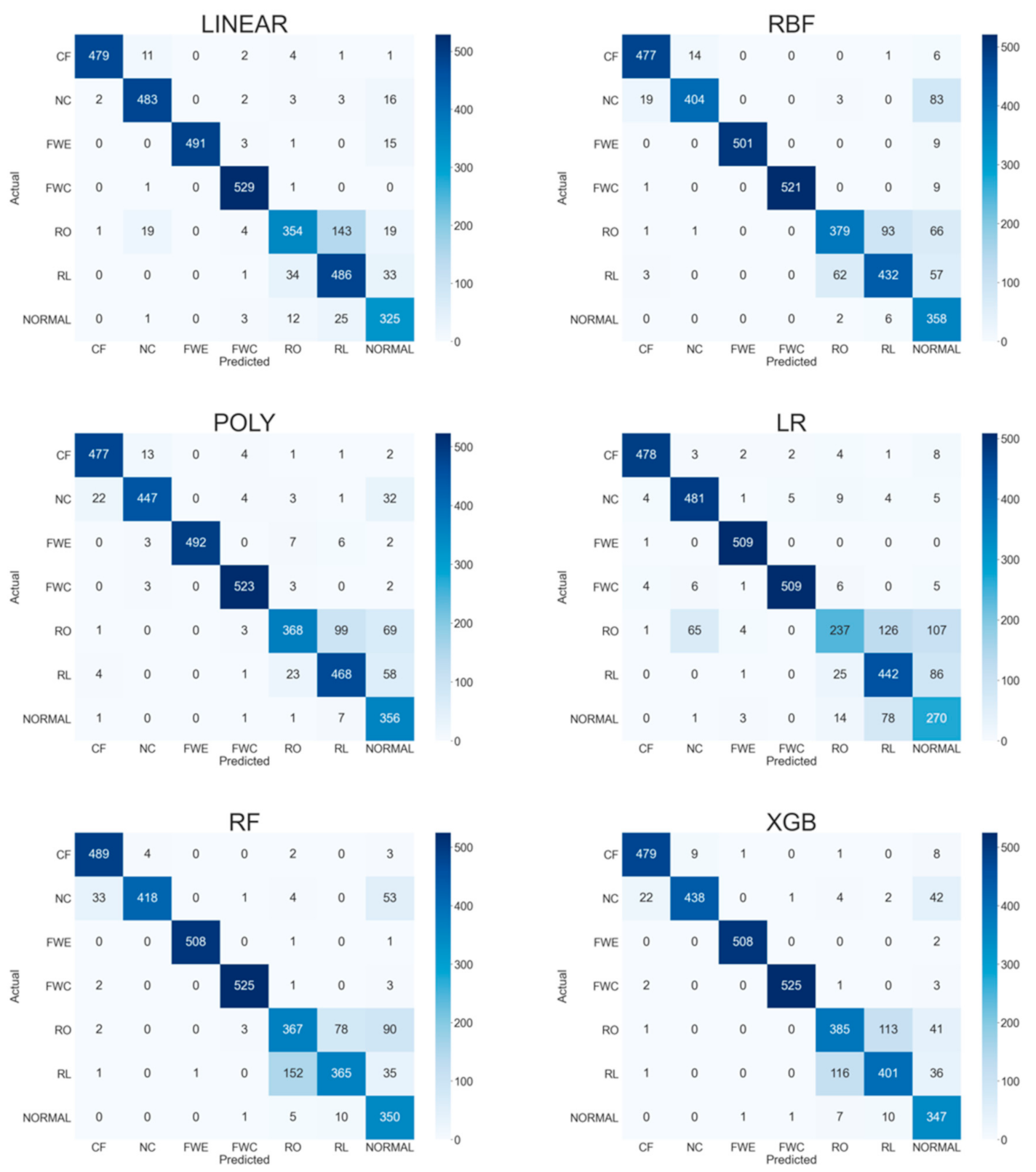
Figure 6 shows the confusion matrices for parameter-tuned classification methods based on the test data. For Linear, one CF, 16 NC, 15 FWE, 19 RO, and 33 RL samples are misclassified as NORMAL. In the system fault, 143 RO samples are misclassified as RL, and 34 RL samples are misclassified as RO. The Linear method does not distinguish the boundaries between RO fault and RL fault well. For the RBF method, six CF, 83 NC, nine FWE, nine FWC, 66 RO, and 57 RL samples are misclassified as NORMAL. With regard to the system fault, 93 RO samples are misclassified as RL, and 62 RL samples are misclassified as RO. The NORMAL samples are well classified themselves, but the boundaries of NORMAL samples overlap with the RO and RL samples. Therefore, the RBF method does not classify RO, RL, and NORMAL well. For the Poly method, two CF, 32 NC, two FWE, two FWC, 69 RO, and 58 RL samples are misclassified as NORMAL. The Poly method, like the RBF method, does not distinguish between system faults and NORMAL well, and several NC samples are misclassified as NORMAL. For the LR method, eight CF, five NC, five FWC, 107 RO, and 86 RL samples are misclassified as NORMAL. With regard to the system fault, 126 RO samples are misclassified as RL, 65 RO samples are misclassified as NC, and 25 RL samples are misclassified as RO. In the NORMAL samples, one, three, 14, and 78 NORMAL samples are misclassified as NC, FWE, RO, and RL, respectively. Similar to the SVM classifier, the performance of the LR method is not effective, especially owing to the misclassification of RO samples as NC. However, the performance of classifying NC samples is better than that of SVM (RBF, Poly). This suggests that the LR method exhibits high performance in classifying the NC faults, but the decision boundaries between NC and RO are overlapped. For the RF method, three CF, 53 NC, one FWE, three FWC, 90 RO, and 35 RL samples are misclassified as NORMAL. With regard to the system fault, 78 RO samples are misclassified as RL, and 152 RL samples are misclassified as RO. Similar to the RBF and Poly methods, the RF method exhibits low performance for NC samples. For the XGB method, eight CF, 42 NC, two FWE, three FWC, 41 RO, and 36 RL samples are misclassified as NORMAL. With regard to the system fault, 113 RO samples are misclassified as RL, and 116 RL samples are misclassified as RO.
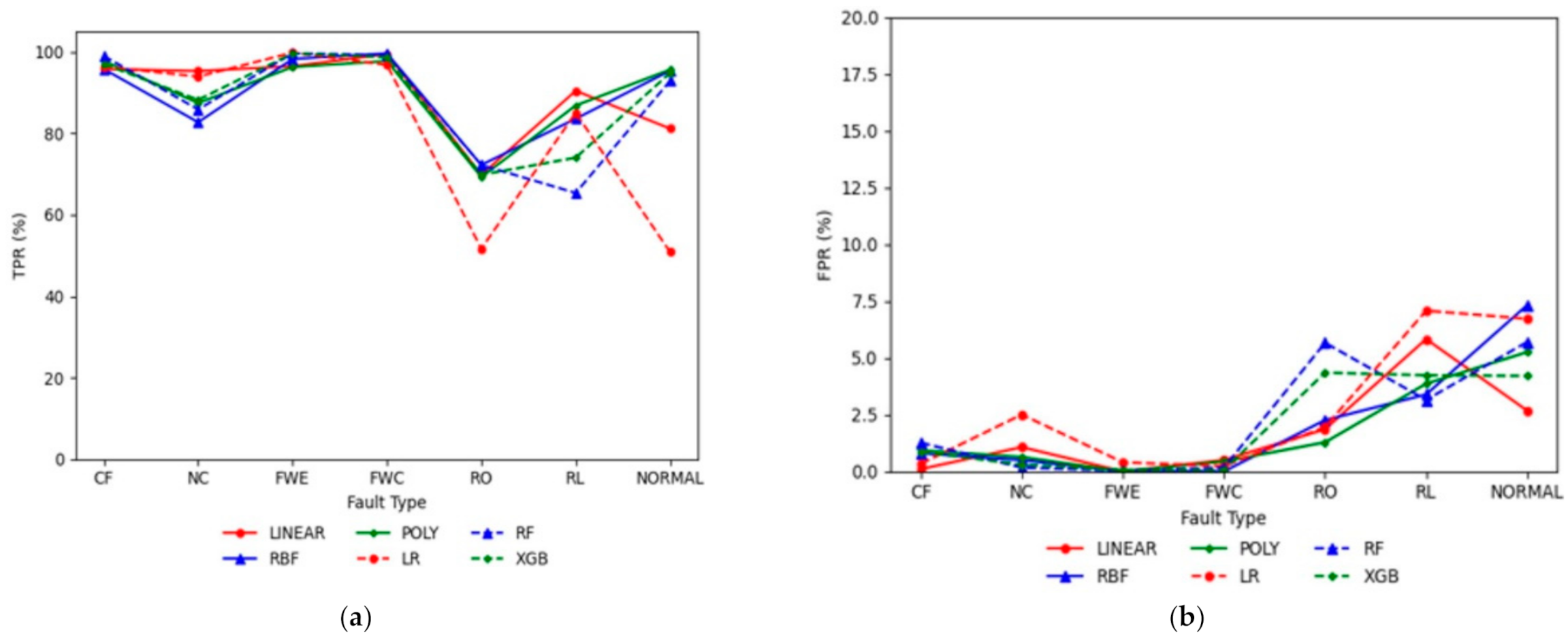
Figure 7a shows the TPR for all the classification methods. The more accurately the model predicts test data, the closer the TPR is to 100%. For CF, FWE, and FWC faults, the TPR values are more than 95% for all the classification methods. For NC, Linear and LR faults are 94.89% and 94.5%, respectively, and are higher than the other classification methods. The reason for the low TPR value is that the NC fault (severity levels 1 and 2) is similar to normal data and is incorrectly determined. RO and RL have relatively low TPR values compared with other faults. The reason for the low TPR value is that RO and RL have little difference between severity levels 1 and 2. For fault detection, TPR has values of 90% or more with Poly, RF, RBF, and XGB. Figure 7b shows the FPR for all the classification methods. The FPR is the ratio of the predicted failed observations. Therefore, the lower the FPR value, the higher the predictive performance.

4.2. Case 2

Case 2 shows the result of the insufficient data, although the data are based on all severity levels. Figure 8 shows 10-fold CV accuracy for Case 2. Compared with Case 1, the average accuracy rates of all the classification methods increased. RB and XGB are the best classification methods, with average accuracy rates of 96.15% and 96.35%, respectively, and Linear, RBF, Poly, and LR exhibited average accuracy rates of 92.07%, 90.82%, 85.43%, and 88.14%, respectively. Although the Case 2 training data set is insufficient, the CV accuracy is higher than in Case 1 because it contains all the severity levels.
Figure 9 shows the 10-fold CV accuracy of the parameter-tuned classification methods pertaining to Case 2. The 10-fold CV accuracy of the Poly method exhibited the highest increase 9.98% to 95.41%. The accuracy of the RF method reduced by 0.2% to 95.95%. For the RF model, the grid search technique may be less accurate than default methods because it determines optimal parameter values within a specified range. The hyperparameters used in Case 2 are listed in Table 6.
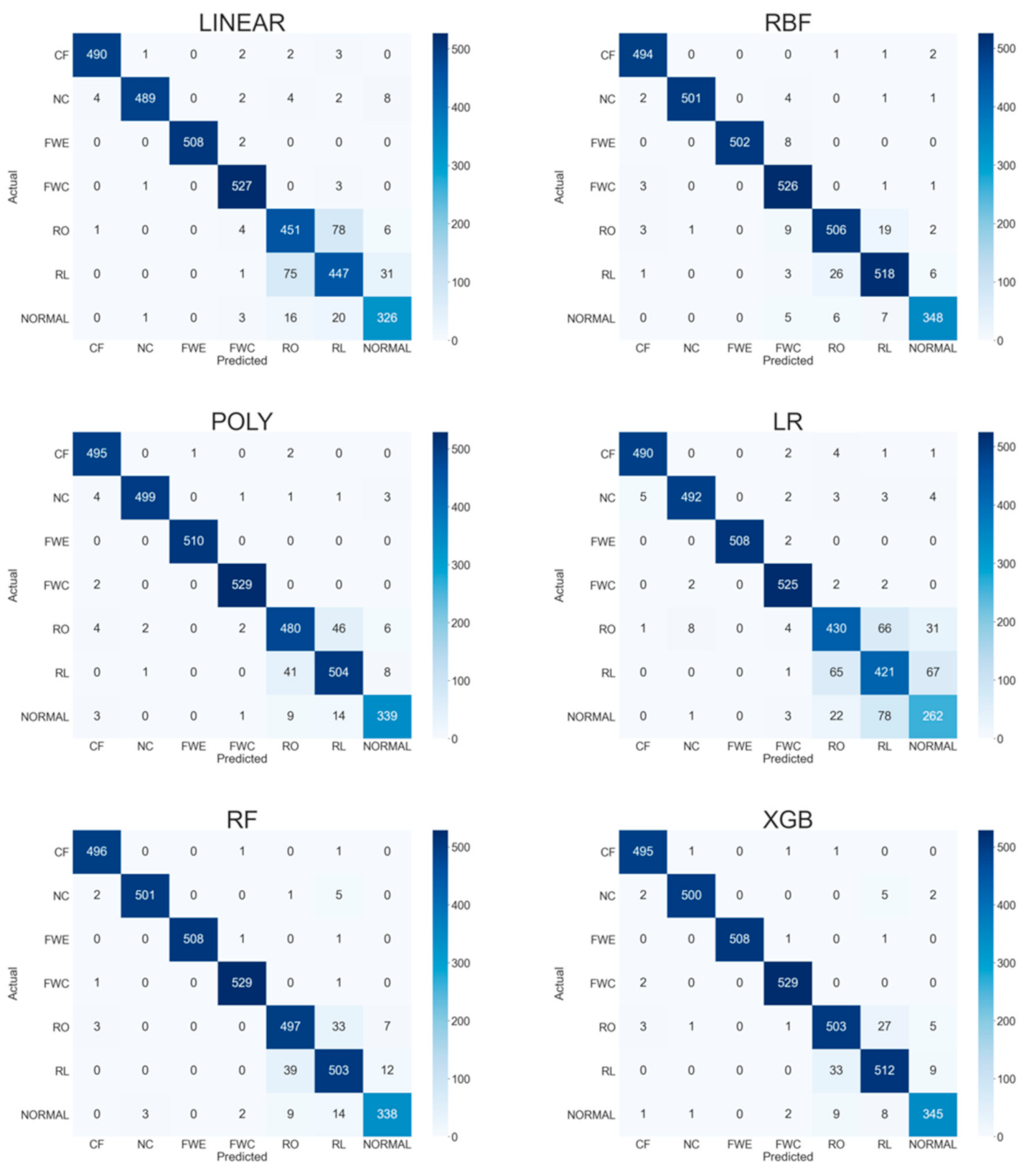
Figure 10 shows the confusion matrices of the parameter-tuned classification methods for Case 2. The test data for Cases 1 and 2 are the same, and the overall performance is better than Case 1. For Linear, 76 RO samples are misclassified as RL, 75 RL samples are misclassified as RO, and 31 RL samples are misclassified as NORMAL. The number of RO and RL classified samples is 451 and 447. Compared with Case 1, RO increased and RL decreased. The number of misclassified samples with regard to the local fault was less than that of Case 1 because NORMAL has decreased. For the RBF method, the TP values of the confusion matrix increased; especially, the TP value of NC samples was 501. NC samples of test data can be better classified as the severity levels (3, 4) are included in the training data set. In the system fault, 19 RO samples are misclassified as RL, and 26 RL samples are misclassified as RO. For the Poly method, the performance is lower than the RBF method, but the TP values of CF, FWE, and FWC have increased. In the system fault, 46 RO samples are misclassified as RL, and 41 RL samples are misclassified as RO. For the LR method, the RO method increased the number of classified samples compared with that of Case 1, but it has a lower TP value than that of the SVM method. For RF and XGB, the TP values for each fault and NORMAL are increased than that for Case 1. With regard to the system fault, the number of samples misclassified as NORMAL, RO, or RL has decreased. Overall, all the methods classify most samples for the local fault, and the RBF method classifies most samples for the system fault.
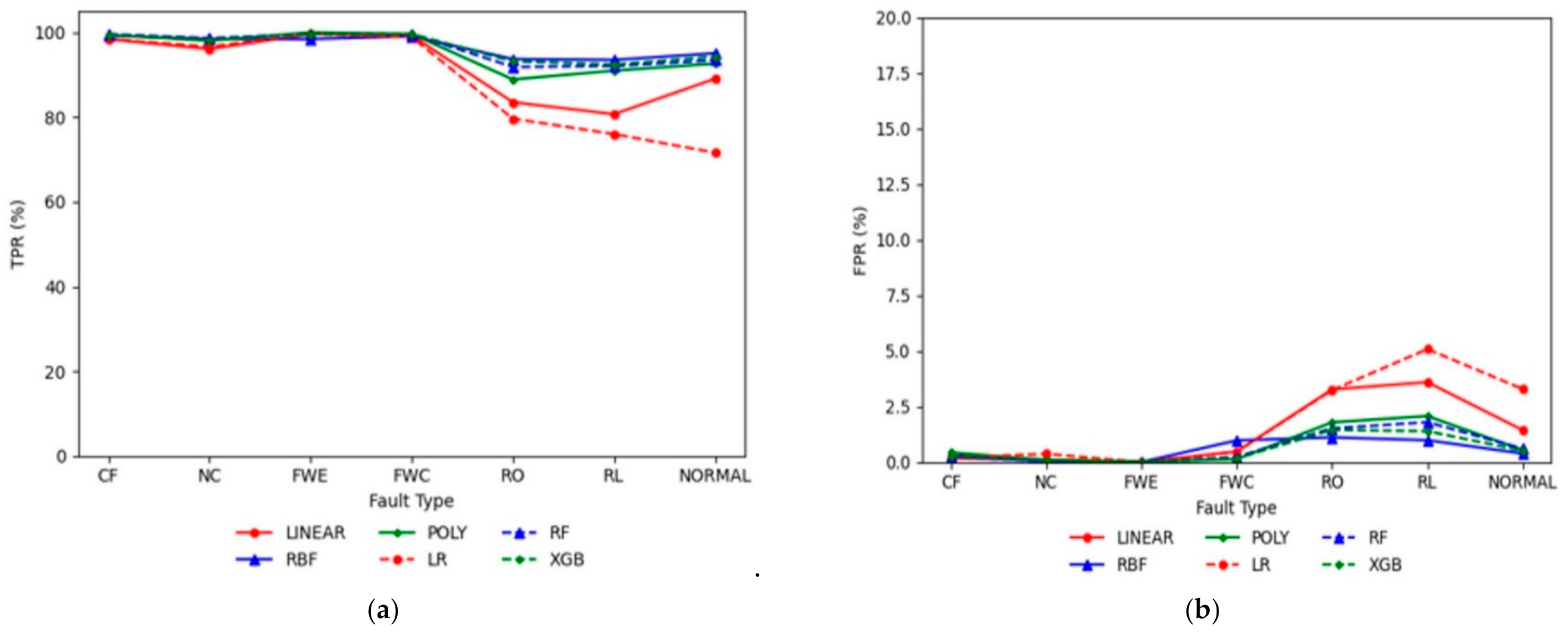
Figure 11a shows TPR values for all the classification methods. The Linear and LR methods exhibit lower TPR values of RO, RL, and NORMAL than the other classification methods. For Linear, the TPR values of CF, NC, FWE, FWC, RO, RL, and NORMAL are 98.39%, 96.07%, 99.61%, 99.25%, 83.52%, 80.69%, and 89.07%, respectively. For LR, the TPR values of CF, NC, FWE, FWC, RO, RL, and NORMAL are 98.39%, 96.66%, 99.61%, 98.87%, 79.63%, 75.99%, and 71.58%, respectively. The TPR values of CF, NC, FWE, and FWC are greater than 98%. Figure 11b shows the FPR values for all the classification methods. The FPR values of RBF, Poly, RF, and XGB are less than 2.5%. The FPR values of the Linear and LR methods are greater than those of the other methods. For Linear, the FPR values of CF, NC, FWE, FWC, RO, RL, and NORMAL are 0.17%, 0.1%, 0.0%, 0.47%, 3.27%, 3.59%, and 1.43%, respectively. For LR, the FPR values of CF, NC, FWE, FWC, RO, RL, and NORMAL are 0.2%, 0.37%, 0.0%, 0.47%, 3.23%, 5.08%, and 3.28%, respectively.

4.3. Case 3

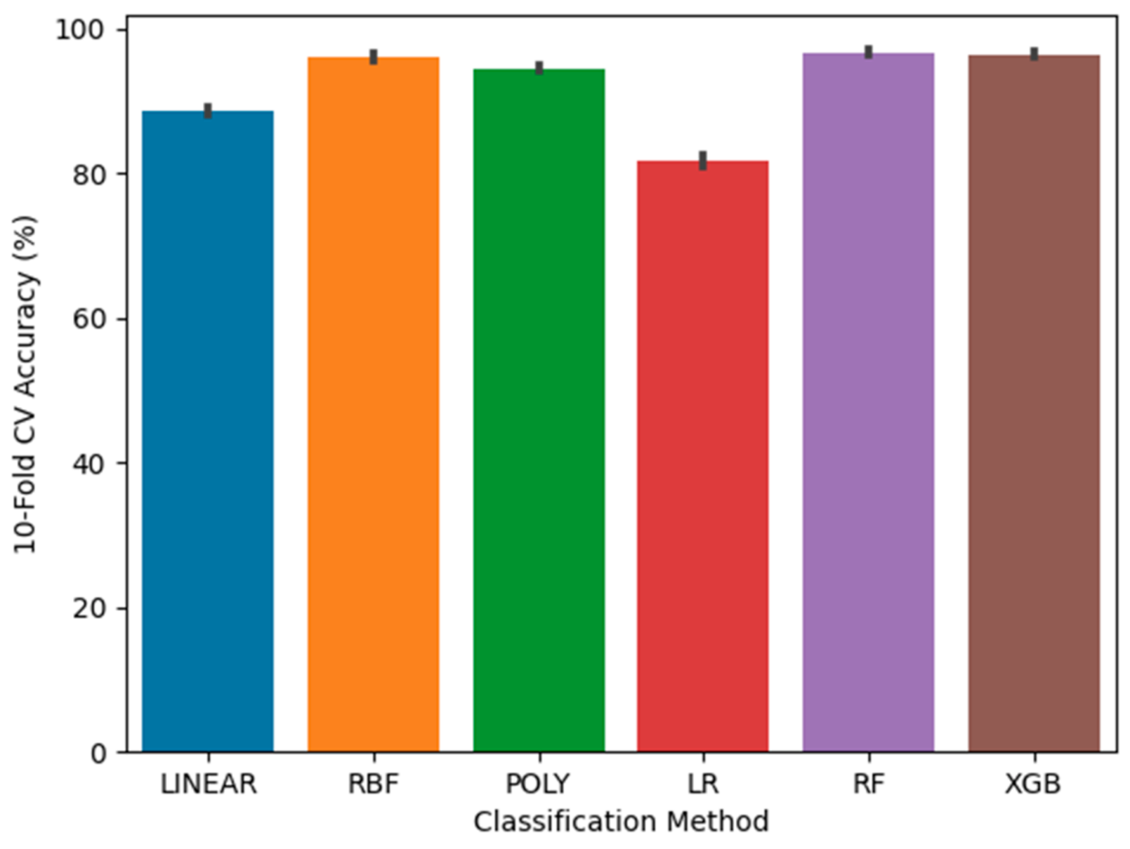
The training data set in Case 3 has sufficient data with severity levels 1 and 2. Figure 12 shows 10-fold CV accuracy for default methods in Case 3. Based on the training accuracy, RF and XGB are the best classification methods, with average accuracy rates of 96.46% and 96.5%, respectively, and Poly is the weakest classification method, with an average accuracy rate of 78.09%. The average accuracy rates of Linear, RBF, and LR are 88.45%, 89.18%, and 81.74%, respectively. The 10-fold CV accuracy of Case 3 increased for all the classification methods compared with that of Case 1, and the accuracy of RF and XGB increased compared with that of Case 2.
Figure 13 shows the 10-fold CV accuracy of the parameter-tuned classification methods pertaining to Case 3. The RF method is the best classification method, with a 0.25% increase to 96.7%, and the LR method is the weakest classification method, with an average accuracy rate of 81.74%. The average accuracy rates of Linear, RBF, Poly, and XGB are 88.76%, 96.1%, 94.54%, and 96.52%, respectively. The hyperparameters used in Case 3 are listed in Table 7.
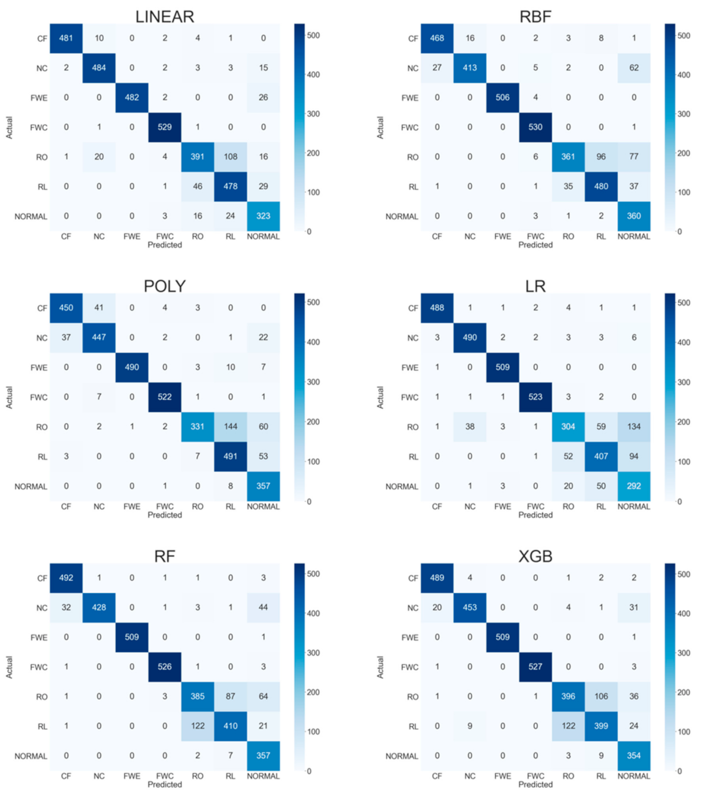
Figure 14 shows the confusion matrices of the parameter-tuned classification methods for Case 3. For Linear, 108 RO samples are misclassified as RL, and 46 RL samples are misclassified as RO. With regard to the system fault, the TP value of RO is 391, which is larger than Case 1. For the RBF method, 62 NC, 77 RO, and 37 RL samples are misclassified as NORMAL. The number of NC and RL misclassified samples decreased compared with that of Case 1. The performance of the Linear method is better than the Poly method, and the number of RO and RL samples, which is misclassified as NORMAL, decreased. For the LR method, the TP value of RO is 304, which increased compared to that of Case 1, and the TP value of RL is 407, which decreased compared to that of Case 1. For RF and XGB, the TP values of the local fault and NORMAL increased, and the number of samples misclassified to NORMAL has decreased.
Figure 15a shows the TPR values for all the classification methods. The Linear and LR methods generate lower TPR values of NORMAL than with the other classification methods. For Linear, the TPR values of CF, NC, FWE, FWC, RO, RL, and NORMAL are 96.59%, 95.09%, 94.51%, 99.62%, 72.41%, 86.28%, and 88.25%, respectively. For LR, the TPR values of CF, NC, FWE, FWC, RO, RL, and NORMAL are 97.99%, 96.27%, 99.8%, 98.49%, 56.3%, 73.47%, and 79.78%, respectively. The TPR values of CF, NC, FWE, and FWC are greater than 80%, and the TPR values of other methods are less than 80%. Figure 15b shows the FPR values for all the classification methods. The FPR values of CF, NC, FWE, and FWC are less than 2.5%. The FPR values of RO, RL, and NORMAL are greater than 2.5%, except RBF and Poly of the RO fault. The FPR values of RO are 0.47% for Poly and 1.38% for RBF.

4.4. Case 4

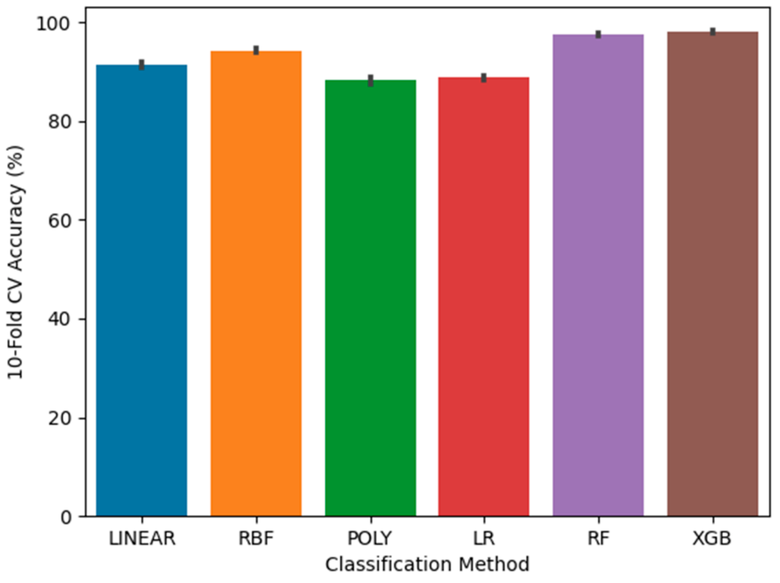
The training data set in Case 4 includes sufficient data with all the severity levels. Figure 16 shows 10-fold CV accuracy for default methods in Case 4. Based on the training accuracy, RF and XGB are the best classification methods, with average accuracy rates of 97.6% and 98%, respectively, and Poly and LR are the weakest classification methods, with average accuracy rates of 88.19% and 88.83%, respectively. For Linear and RBF, the average accuracy rates are 91.4% and 94.18%, respectively.
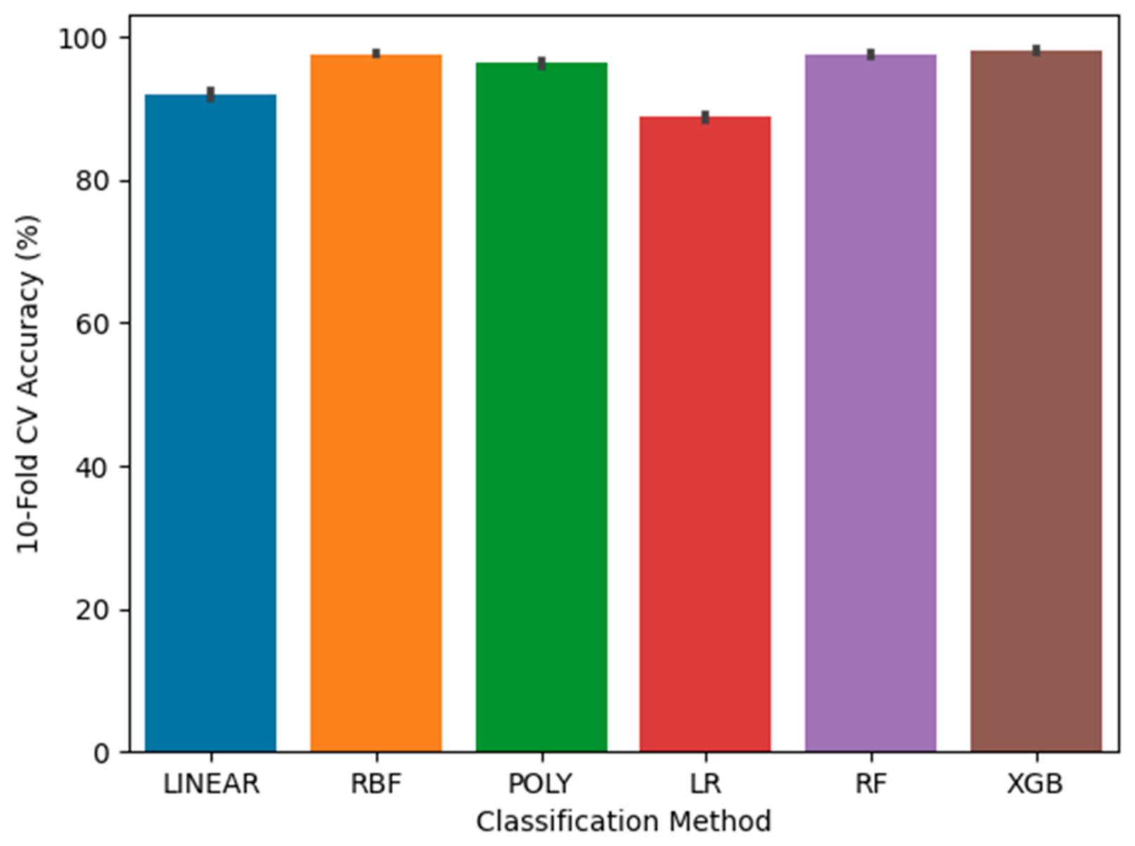
Figure 17 shows the 10-fold CV accuracy of the parameter-tuned classification methods for Case 4. The XGB method is the best classification method, with a 0.07% increase to 98.08%, and the LR method is the weakest classification method, with an average accuracy rate of 88.83%. For Linear, RBF, Poly, and RF, the average accuracy rates are 91.87%, 97.7%, 96.43%, and 97.62%, respectively. The hyperparameters used in Case 4 are listed in Table 8.
Figure 18 shows the confusion matrices of the parameter-tuned classification methods for Case 4. For Linear, 71 RO samples are misclassified as RL, 72 RL samples are misclassified as RO, and the TP value is not significantly different from that of Case 2. For the RBF method, 21 RO samples are misclassified as RL, and 15 RL samples are misclassified as RO. The TP values of all samples are greater than those of Case 3. For the Poly method, 36 RO samples are misclassified as RL, and 24 RL samples are misclassified as RO. The TP values of RO and RL are larger than that of other cases. For the LR method, the TP values for all the samples are similar to Case 2 and are larger than those for Case 3. For the RF and XGB methods, the TP values pertaining to the system fault have slightly increased.
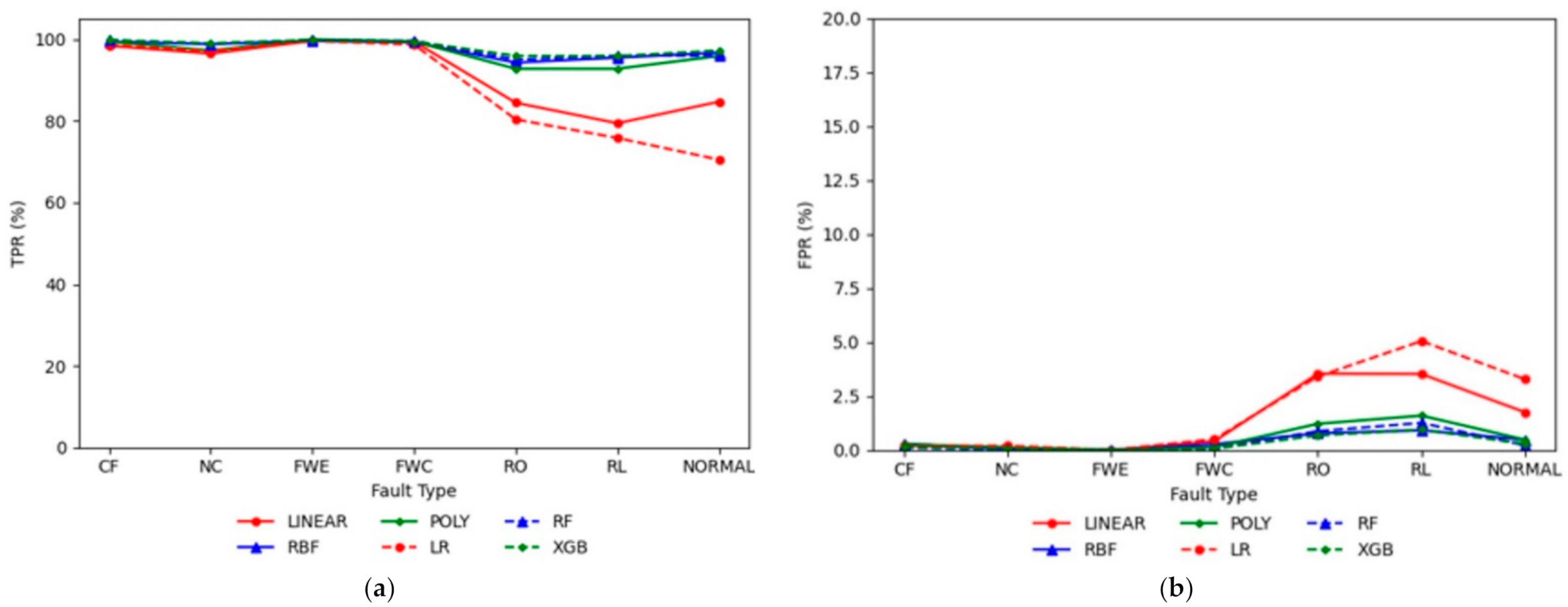
Figure 19a shows the TPR values for all the classification methods. The Linear and LR methods generate lower TPR values of RO, RL, and NORMAL compared to the other classification methods. For Linear, the TPR values of CF, NC, FWE, FWC, RO, RL, and NORMAL are 98.39%, 96.46%, 99.61%, 99.44%, 84.44%, 79.42%, and 84.7%, respectively. For LR, the TPR values of CF, NC, FWE, FWC, RO, RL, and NORMAL are 98.89%, 97.05%, 99.61%, 98.68%, 80.37%, 75.81%, and 70.49%, respectively. For other methods, all the TPR values are greater than 95%. Figure 19b shows the FPR values of all the classification methods. The Linear and LR methods generate larger FPR values of RO, RL, and NORMAL than other classification methods. For Linear, the FPR values of CF, NC, FWE, FWC, RO, RL, and NORMAL are 0.2%, 0.1%, 0.0%, 0.4%, 3.54%, 3.52%, and 1.75%, respectively. For LR, the FPR values of CF, NC, FWE, FWC, RO, RL, and NORMAL are 0.17%, 0.2%, 0.5%, 3.4%, 5.04%, and 3.28%, respectively. For other methods, all the FPR values are less than 2.5%.

5. Conclusions

A data-driven FDD method was presented in this study. The proposed strategy was validated using the ASHRAE 1043-RP data and considered the FDD task as a multi-case classification problem. Six machine learning classification methods were applied to FDD in a chiller. For the multi-case, we created four groups: Case 1 (training data: 30%, severity levels: 1 and 2), Case 2 (training data: 30%, severity levels: 1, 2, 3, and 4), Case 3 (training data: 70%, severity levels: 1 and 2), Case 4 (training data: 70%, severity levels: 1, 2, 3, and 4). Cases 1 and 2 defined a situation where the training data were insufficient, and cases 3 and 4 defined a situation where the training data were sufficient. In addition, situations with different severity levels are classified based on each case. The simulation approach was validated using default and parameter-tuned classification methods. The results showed that the classification methods can detect faults and diagnose chiller systems. Based on each case, the results are as follows:
(1)
Case 1: RBF and RF are the best classification methods, with average accuracy rates of 95.43% and 95.64%. For the local fault, the TPR values of Linear and LR are greater than 95%, and the FPR values of RBF, Poly, RF, and XGB are less than 2.0%. For fault detection, the RBF, Poly, RF, and XGB methods predicted correctly, and for fault diagnostics, Linear and LR predicted correctly. Pertaining to the system fault, TPR and FPR values are poor for all the classification methods. For fault detection and diagnostics, all the classification methods predicted incorrectly.
(2)
Case 2: XGB is the best classification method, with an average accuracy rate of 96.55%. For the local fault, the TPR values of all the classification methods are greater than 95%, and the FPR values of all the classification methods are lower than 2.0%. For fault detection and diagnostics, all the classification methods predicted correctly. Pertaining to the system fault, the TPR values of RBF, Poly, RF, and XGB are greater than 90%, and the FPR values of RBF, Poly, RF, and XGB are less than 2.5%. For fault detection and diagnostics, RBF, Poly, RF, and XGB predicted correctly.
(3)
Case 3: RF is the best classification method, with an average accuracy rate of 96.7%. For the local fault, the TPR values of Linear and LR are greater than 94%, and the FPR values of all the classification methods are lower than 2.5%. In fault detection, all the classification methods predicted correctly, and in fault diagnostics, Linear and LR predicted correctly. For the system fault, the TPR and FPR values of all the classification methods are poor.
(4)
Case 4: XGB is the best classification method, with an average accuracy rate of 98.08%. For the local fault, the TPR values of all the classification methods are greater than 95%, and in Case 2, the FPR values of all the classification methods are ~0%, which is lower than that of Case 2. In fault detection and diagnostics, all the classification methods predicted correctly. With regard to the system fault, the TPR values of RBF, Poly, RF, and XGB are greater than 94%, and the FPR values of RBF, Poly, RF, and XGB are less than 1.6%. In fault detection and diagnostics, RBF, Poly, RF, and XGB predicted correctly.
For the local faults, the results show high accuracy in all cases, and they can be accurately classified with insufficient data and limited severity levels. Especially, when the severity levels are limited, the Linear and LR methods have high accuracy compared to other methods. For the system faults, it is difficult for all methods to classify the system faults in Case 1, 2, and 3. These results indicate that determining the system fault requires a larger amount of training data than the test data and also requires information about all severity levels. These results show that the RF and XGB methods have high accuracy for all the cases. In the previous studies, since there is no difference between the severity levels or the amount of data for training data and test data, it is difficult to apply when the amount of fault data is insufficient or biased, such as in the industrial field. Our FDD strategy derives an optimal model for limited fault data or severity levels. When constructing the data-driven methods, it will be a good feed for determining the constituent model for each fault type or severity level. Also, it is simple and scalable using the Python library, and we plan to incorporate this FDD strategy into a test bed. The results of the proposed FDD strategy enable us to effective perform fault diagnosis on insufficient data set in the industrial field, In the future, a virtual chiller simulator will be built to obtain fault data according to fault scenarios, and we will verify the performance of the proposed FDD strategy using the fault data.

Author Contributions

Conceptualization, I.K. and W.K.; methodology, W.K.; software, I.K.; validation, I.K.; formal analysis, I.K.; investigation, I.K.; resources, W.K.; data curation, I.K.; writing—original draft preparation, I.K.; writing—review and editing, W.K.; visualization, I.K.; supervision, W.K.; project administration, W.K.; funding acquisition, W.K. All authors have read and agreed to the published version of the manuscript.

Funding

This research was financially supported by Chonnam National University (Grant number: 2020-1992) and the National Research Council of Science & Technology (NST) grant by the Korea government (MSIT) (No. CRC-15-05-ETRI).

Institutional Review Board Statement

Not applicable.

Informed Consent Statement

Not applicable.

Data Availability Statement

Data sharing not applicable.

Conflicts of Interest

The authors declare no conflict of interest.

Nomenclature

TP true positive
TN true negative
FP false positive
FN false negative
TPR true positive rate
FPR false positive rate
LV level for severity
sgn sign function
w , w T weight vector for SVM method
X training data
x , x input vector for training data
b bias of hyperplane in SVM method
C control tradeoff in SVM method
ζ i distance from decision boundary
γ hyperparameter gamma in RBF and Polynomial methods
d degree of polynomial method
θ parameter for polynomial method
K x , x kernel function for input vector in SVM method
σ X sigmoid logistic function for logistic regression method
p ^ output data for logistic regression method
Y ^ prediction value for XGB method
f k regularization function for XGB method
F functional space for XGB method
l Y ^ , Y loss function for XGB method
TEOTemperature of evaporator water out
TCOTemperature of condenser water out
FWCFlow rate of condenser water
TRCSaturated Refrigerant temperature in condenser
TR_disRefrigerant discharge temperature
PO_feedPressure of oil feed
VEEvaporator valve position
TWITemperature of city water in

References

  1. Katipamula, S.; Brambley, M.R. Methods for fault detection, diagnostics, and prognostics for building systems—A review, part I. HvacR Res. 2005, 11, 3–25. [Google Scholar] [CrossRef]
  2. Gordon, J.M.; Ng, K.C.; Chua, H.T. Centrifugal chillers, thermodynamic modelling and a diagnostic case study. Int. J. Refrig. 1995, 18, 253–257. [Google Scholar] [CrossRef]
  3. Han, H.; Gu, B.; Hong, Y.; Kang, J. Automated FDD of multiple-simultaneous faults (MSF) and the application to building chillers. Energy Build. 2011, 43, 2524–2532. [Google Scholar] [CrossRef]
  4. Comstock, M.C.; Braun, J.E.; Groll, E.A. A survey of common faults for chillers/Discussion. Ashrae Trans. 2002, 108, 819. [Google Scholar]
  5. Comstock, M.C.; Braun, J.E.; Bernhard, R. Experimental Data from Fault Detection and Diagnostic Studies on a Centrifugal Chiller; Purdue University: West Lafayette, IN, USA, 1999. [Google Scholar]
  6. Wang, S.; Cui, J. Sensor-fault detection, diagnosis and estimation for centrifugal chiller systems using principal-component analysis method. Appl. Energy 2005, 82, 197–213. [Google Scholar] [CrossRef]
  7. Han, H.; Gu, B.; Kang, J.; Li, Z.R. Study on a hybrid SVM model for chiller FDD applications. Appl. Therm. Eng. 2011, 31, 582–592. [Google Scholar] [CrossRef]
  8. Zhao, Y.; Wang, S.; Xiao, F. A statistical fault detection and diagnosis method for centrifugal chillers based on exponentially-weighted moving average control charts and support vector regression. Appl. Therm. Eng. 2013, 51, 560–572. [Google Scholar] [CrossRef]
  9. Hu, Y.; Chen, H.; Xie, J.; Yang, X.; Zhou, C. Chiller sensor fault detection using a self-adaptive principal component analysis method. Energy Build. 2012, 54, 252–258. [Google Scholar] [CrossRef]
  10. Yan, K.; Ji, Z.; Shen, W. Online fault detection methods for chillers combining extended kalman filter and recursive one-class SVM. Neurocomputing 2017, 228, 205–212. [Google Scholar] [CrossRef] [Green Version]
  11. Fan, Y.; Cui, X.; Han, H.; Lu, H. Feasibility and improvement of fault detection and diagnosis based on factory-installed sensors for chillers. Appl. Therm. Eng. 2020, 164, 114506. [Google Scholar] [CrossRef]
  12. Han, H.; Cui, X.; Fan, Y.; Qing, H. Least squares support vector machine (LS-SVM)-based chiller fault diagnosis using fault indicative features. Appl. Therm. Eng. 2019, 154, 540–547. [Google Scholar] [CrossRef]
  13. Garreta, R.; Moncecchi, G. Learning Scikit-Learn: Machine Learning in Python; Packt Publishing Ltd: Birmingham, UK, 2013. [Google Scholar]
  14. Chen, T.; Guestrin, C. Xgboost: A scalable tree boosting system. In Proceedings of the 22nd ACM SIGKDD International Conference on Knowledge Discovery and Data Mining, San Francisco, CA, USA, 13–17 August 2016; Association for Computing Machinery : New York, NY, USA, 2016; pp. 785–794. [Google Scholar]
  15. Li, G.; Hu, Y.; Chen, H.; Shen, L.; Li, H.; Hu, M.; Liu, J.; Sun, K. An improved fault detection method for incipient centrifugal chiller faults using the PCA-R-SVDD algorithm. Energy Build. 2016, 116, 104–113. [Google Scholar] [CrossRef]
  16. Zhao, Y.; Wang, S.; Xiao, F. Pattern recognition-based chillers fault detection method using support vector data description (SVDD). Appl. Energy 2013, 112, 1041–1048. [Google Scholar] [CrossRef]
  17. Bishop, C.M. Pattern Recognition and Machine Learning; Springer: Berlin/Heidelberg, Germany, 2006. [Google Scholar]
  18. James, G.; Witten, D.; Hastie, T.; Tibshirani, R. An Introduction to Statistical Learning; Springer: New York, NY, USA, 2013. [Google Scholar]
  19. Witten, I.H.; Frank, E.; Hall, M.A.; Pal, C.J. Practical Machine Learning Tools and Techniques; Morgan Kaufmann: Burlington, MA, USA, 2005; p. 578. [Google Scholar]
  20. Vapnik, V.; Vapnik, V. Statistical Learning Theory; Wiley: New York, NY, USA, 1998; Volume 1, p. 2. [Google Scholar]
  21. Support Vector Machines. Available online: https://scikit-learn.org/stable/modules/svm.html (accessed on 31 December 2020).
  22. Hosmer, D.W., Jr.; Lemeshow, S.; Sturdivant, R.X. Applied Logistzic Regression; John Wiley & Sons: Hoboken, NJ, USA, 2013. [Google Scholar]
  23. Yu, F.W.; Ho, W.T.; Chan, K.T.; Sit, R.K. Logistic regression-based optimal control for air-cooled chiller. Int. J. Refrig. 2018, 85, 200–212. [Google Scholar] [CrossRef]
  24. Wackerly, D.; Mendenhall, W.; Scheaffer, R.L. Mathematical Statistics with Applications; Cengage Learning: Boston, MA, USA, 2014. [Google Scholar]
  25. Casella, G.; Berger, R.L. Statistical Inference; Cengage Learning: Boston, MA, USA, 2021. [Google Scholar]
  26. Biau, G.; Scornet, E. A random forest guided tour. Test 2016, 25, 197–227. [Google Scholar] [CrossRef] [Green Version]
  27. Maroco, J.; Silva, D.; Rodrigues, A.; Guerreiro, M.; Santana, I.; de Mendonça, A. Data mining methods in the prediction of Dementia: A real-data comparison of the accuracy, sensitivity and specificity of linear discriminant analysis, logistic regression, neural networks, support vector machines, classification trees and random forests. BMC Res. Notes 2011, 4, 299. [Google Scholar] [CrossRef] [PubMed] [Green Version]
  28. Breiman, L. Random forests. Mach. Learn. 2001, 45, 5–32. [Google Scholar] [CrossRef] [Green Version]
  29. Yu, F.W.; Ho, W.T.; Chan, K.T.; Sit, R.K.; Yang, J. Economic analysis of air-cooled chiller with advanced heat rejection. Int. J. Refrig. 2017, 73, 54–64. [Google Scholar] [CrossRef]
  30. Chakraborty, D.; Elzarka, H. Early detection of faults in HVAC systems using an XGBoost model with a dynamic threshold. Energy Build. 2019, 185, 326–344. [Google Scholar] [CrossRef]
  31. Comstock, M.C.; Braun, J.E.; Bernhard, R. Development of Analysis Tools for the Evaluation of Fault Detection and Diagnostics in Chillers; Purdue University: West Lafayette, IN, USA, 1999. [Google Scholar]
  32. Li, D.; Hu, G.; Spanos, C.J. A data-driven strategy for detection and diagnosis of building chiller faults using linear discriminant analysis. Energy Build. 2016, 128, 519–529. [Google Scholar] [CrossRef]
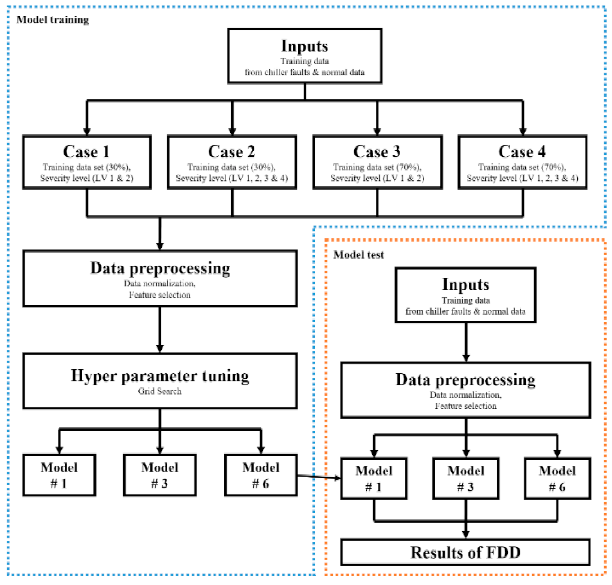
Figure 1. Schematic of proposed FDD strategy.
Energies 14 01945 g001
Figure 2. Trends of the PO_feed dataset.
Energies 14 01945 g002
Figure 3. Schematic of the random forest model.
Energies 14 01945 g003
Figure 4. 10-fold CV accuracy for default classification methods (Case 1).
Energies 14 01945 g004
Figure 5. 10-fold CV accuracy for parameter-tuned classification methods (Case 1).
Energies 14 01945 g005
Figure 6. Confusion matrices for parameter-tuned classification methods (Case 1).
Energies 14 01945 g006
Figure 7. TPR and FPR values for each classification method (Case 1): (a) TPR; (b) FPR.
Energies 14 01945 g007
Figure 8. 10-fold CV accuracy for default classification methods (Case 2).
Energies 14 01945 g008
Figure 9. 10-fold CV accuracy for parameter-tuned classification methods (Case 2).
Energies 14 01945 g009
Figure 10. Confusion matrices for parameter-tuned classification methods (Case 2).
Energies 14 01945 g010
Figure 11. TPR and FPR values for each classification method (Case 2): (a) TPR; (b) FPR.
Energies 14 01945 g011
Figure 12. 10-fold CV accuracy for default classification methods (Case 3).
Energies 14 01945 g012
Figure 13. 10-fold CV accuracy for parameter-tuned classification methods (Case 3).
Energies 14 01945 g013
Figure 14. Confusion matrices for parameter-tuned classification methods (Case 3).
Energies 14 01945 g014
Figure 15. TPR and FPR values for each classification method (Case 3): (a) TPR; (b) FPR.
Energies 14 01945 g015
Figure 16. 10-fold CV accuracy for default classification methods (Case 4).
Energies 14 01945 g016
Figure 17. 10-fold CV accuracy for parameter-tuned classification methods (Case 4).
Energies 14 01945 g017
Figure 18. Confusion matrices for parameter-tuned classification methods (Case 4).
Energies 14 01945 g018
Figure 19. TPR and FPR values for each classification method (Case 1): (a) TPR; (b) FPR.
Energies 14 01945 g019
Table 1. Confusion matrix for FWC.
Predicted Class
CFNCFWEFWCRORLNORMAL
Actual ClassCFTNTNTNFPTNTNTN
NCTNTNTNFPTNTNTN
FWETNTNTNFPTNTNTN
FWCFNFNFNTPFNFNFN
ROTNTNTNFPTNTNTN
RLTNTNTNFPTNTNTN
NORMALTNTNTNFPTNTNTN
Table 2. Fault types and severity levels.
Fault TypesLV 1LV 2LV 3LV 4Methods
RO10%20%30%40%Increasing the refrigerant charge by weight
RL10%20%30%40%Reducing the refrigerant charge by weight
NC1%2%3%5%Adding nitrogen by volume
FWE10%20%30%40%Reducing water flow by percentage
FWC10%20%30%40%Reducing water flow by percentage
CF12%20%30%45%Plugging tubes by percentage
Table 3. Input and output features of the dataset.
DatasetFeatures
Input (x value)TEO, TCO, FWC, TRC, TR_dis, PO_feed, VE, and TWI
Output (y value)Fault types (RO, RL, NC, FWE, FWC, CF, and NORMAL)
Table 4. Case scenarios of the dataset.
DatasetCase 1Case 2Case 3Case 4
Training data1948350745468183
Test Data3508350835083508
Total Data5456701580541,1691
Table 5. Hyperparameter tuning for each classification method (Case 1).
ModelsHyperparametersRange of ValuesOptimal Values
LinearRegularization parameter, C[0.001, 0.01, …, 1000, 10,000]100
RBFRegularization parameter, C[1, 10, 100, 1000, 10,000]100
Kernel coefficient, γ [0.0001, 0.001, 0.01, 0.1, 1]1
PolyRegularization parameter, C[0.001, 0.01, …, 1000, 10,000]1000
Kernel coefficient, γ [0.0001, 0.001, 0.01, 0.1, 1]0.1
LRInverse of regularization strength, C[0.001, 0.01, …, 1000, 10,000]10
RFMaximum depth of the tree, max_depth[10, 20, …, 80, 90, 100]80
Number of trees, n_estimators[100, 200, …, 800, 900, 1000]1000
XGBBoosting learning rate, learning_rate[0.001, 0.005, …, 0.1, 0.5, 1]1
Maximum depth of the tree, max_depth[1, 2, 3, 4, 5, 6, 7, 8, 9, 10]7
Minimum sum of instance weight, min_child_weight[1, 10, 100, 1000]1
Table 6. Hyperparameter tuning for each classification method (Case 2).
ModelsHyperparametersRange of ValuesOptimal Values
LinearRegularization parameter, C[0.001, 0.01,   , 1000, 10,000]10
RBFRegularization parameter, C[1, 10, 100, 1000, 10,000]1000
Kernel coefficient, γ [0.0001, 0.001, 0.01, 0.1, 1]1
PolyRegularization parameter, C[0.001, 0.01,   , 1000, 10,000]1000
Kernel coefficient, γ [0.0001, 0.001, 0.01, 0.1, 1]0.1
LRInverse of regularization strength, C[0.001, 0.01,   , 1000, 10,000]1
RFMaximum depth of the tree, max_depth[10, 20,   , 80, 90, 100]20
Number of trees, n_estimators[100, 200,   , 800, 900, 1000]200
XGBBoosting learning rate, learning_rate[0.001, 0.005, , 0.1, 0.5, 1]0.5
Maximum depth of the tree, max_depth[1, 2, 3, 4, 5, 6, 7, 8, 9, 10]7
Minimum sum of instance weight, min_child_weight[1, 10, 100, 1000]1
Table 7. Hyperparameter tuning for each classification method (Case 3).
ModelsHyperparametersRange of ValuesOptimal Values
LinearRegularization parameter, C[0.001, 0.01,   , 1000, 10,000]100
RBFRegularization parameter, C[1, 10, 100, 1000, 10,000]100
Kernel coefficient, γ [0.0001, 0.001, 0.01, 0.1, 1]1
PolyRegularization parameter, C[0.001, 0.01,   , 1000, 10,000]100
Kernel coefficient, γ [0.0001, 0.001, 0.01, 0.1, 1]1
LRInverse of regularization strength, C[0.001, 0.01,   , 1000, 10,000]1
RFMaximum depth of the tree, max_depth[10, 20,   , 80, 90, 100]50
Number of trees, n_estimators[100, 200,   , 800, 900, 1000]600
XGBBoosting learning rate, learning_rate[0.001, 0.005, , 0.1, 0.5, 1]0.5
Maximum depth of the tree, max_depth[1, 2, 3, 4, 5, 6, 7, 8, 9, 10]9
Minimum sum of instance weight, min_child_weight[1, 10, 100, 1000]1
Table 8. Hyperparameter tuning for each classification method (Case 4).
ModelsHyperparametersRange of ValuesOptimal Values
LinearRegularization parameter, C[0.001, 0.01,   , 1000, 10,000]10,000
RBFRegularization parameter, C[1, 10, 100, 1000, 10,000]1000
Kernel coefficient, γ [0.0001, 0.001, 0.01, 0.1, 1]1
PolyRegularization parameter, C[0.001, 0.01,   , 1000, 10,000]10
Kernel coefficient, γ [0.0001, 0.001, 0.01, 0.1, 1]1
LRInverse of regularization strength, C[0.001, 0.01,   , 1000, 10,000]1
RFMaximum depth of the tree, max_depth[10, 20,   , 80, 90, 100]40
Number of trees, n_estimators[100, 200,   , 800, 900, 1000]100
XGBBoosting learning rate, learning_rate[0.001, 0.005, , 0.1, 0.5, 1]0.5
Maximum depth of the tree, max_depth[1, 2, 3, 4, 5, 6, 7, 8, 9, 10]8
Minimum sum of instance weight, min_child_weight[1, 10, 100, 1000]1
Publisher’s Note: MDPI stays neutral with regard to jurisdictional claims in published maps and institutional affiliations.