Regional Pole Placers of Power Systems under Random Failures/Repair Markov Jumps

Abstract

This paper deals with a discrete-time stochastic control model design for random failure prone and maintenance in a single machine infinite bus (SMIB) system. This model includes the practical values of failure/repair rate of transmission lines and transformers. The probability matrix is, therefore, calculated accordingly. The model considers two extreme modes of operations: the most reliable mode and the least reliable contingency case. This allows the control design which stochastically stabilizes the system under jump Markov disturbances. For adequate transient response, the proposed state feedback power system stabilizer (PSS) achieves a desired settling time and damping ratio by placing the closed-loop poles in a desired region. The control target should also be satisfied for load variations in either mode of operation. A sufficient condition is developed to achieve the control objectives via solving a set of linear matrix inequalities (LMI). Using simulation, the performance of the designed controller is tested for the system that prone to random failure/maintenance under various loading conditions. Simulation results reveal that the closed-loop poles reside within the desired region satisfying the required settling time and damping ratio under the aforementioned disturbances. The contributions of the paper are summarized as follows: (1) modeling of transition probability matrix under Markov Jumps using practical data, (2) designing a controller by compelling the closed poles into the desired region to achieve adequate dynamic performance under different load varying conditions.

1. Introduction

Power systems are subject to spontaneous disturbances which result in rotor angle oscillations of synchronous generators. Such oscillations might grow, causing loss of synchronism and system separation, which results in great loss of national economy. The resulting oscillations are damped by power system stabilizers(PSS), injecting a stabilizing signal to the excitation channel. Different designs of PSS exist in numerous literature [1,2,3,4].

Research efforts considering reliable power system stabilization in case of failure of the PSS is minimal. One approach is to control the synchronous generator by two controllers, such as the governor and the excitation control. Reliable stabilization is achieved when either controller fails or both are sound as given in [5]. In such an approach, the system dynamics is governed by ordinary differential equations.

Power systems are subject to random parameter changes, which can be triggered by random component failures, repairs, or sudden changes in the operating point due to the changes in the loads and the integration of distributed energy resources [6]. Ref. [7] has used a multi-objective function that is solved using nonlinear simplex function in order to design the power system stabilizer. A power system stabilizer for multi-operating conditions is designed using the probabilistic Eigen values in [8]. The evaluation of system reliability is carried out by using Markov process, or Monte Carlo method [9,10,11,12,13]. Implementing the Monte Carlo method for simulation has some limitations, such as slow convergence rate, and high computational complexity. Kai Hou et al. proposed a more efficient Markov chain-based sequential analytical model for small scale system [14]. Short-term reliability analysis is performed using a multi-state Markov model in [15]. Hence, this paper aims to design a fast operational reliability analyzing model based on an analytical approach. The proposed model is based on the Markov chain, and is modeled with the assumption that the equipment failure rate has an exponential characteristic. Furthermore, this paper also presents a Markov state transition probability matrix, which is obtained based on historical practical data of power system operation. Ref. [16] considers power system stabilization under a series of lightning strokes. An adaptive fuzzy sliding mode control for power system stabilizer is designed to overcome possible chattering due to uncertain system dynamics and improve the power system efficiency and performance [17].

System dynamics under random changes can be described by differential equations. Power system stabilization under abrupt load changes modelled by a Markov chain is given in [18]; cascading failure is tackled in [19,20]. This paper presents the design and tests of regional pole placer-based discrete-time stochastic control model under random changes in a SMIB system. The main originality and contributions of this paper are:

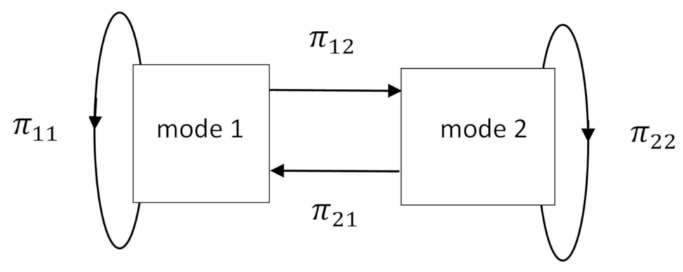
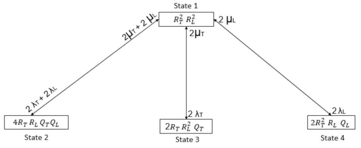
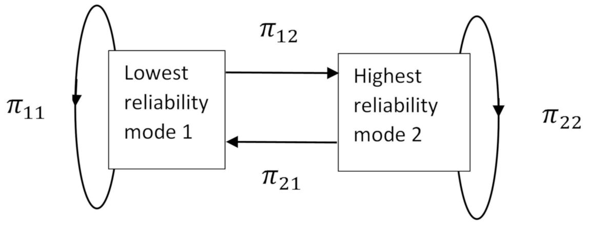
• Two extreme cases, such as the most reliable and the least reliable modes of a SMIB system, are considered. The transition probability matrix of the SMIB system is obtained from the practical results of line/transformer failure repair rates.
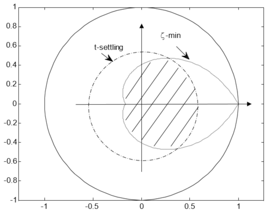
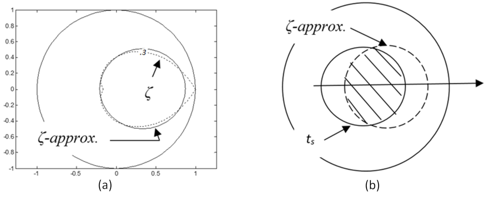
• A simple state feedback PSS design is developed in the framework of LMI to achieve stochastic stability in terms of settling time and damping ratio (regional pole placement for the discrete-time system).
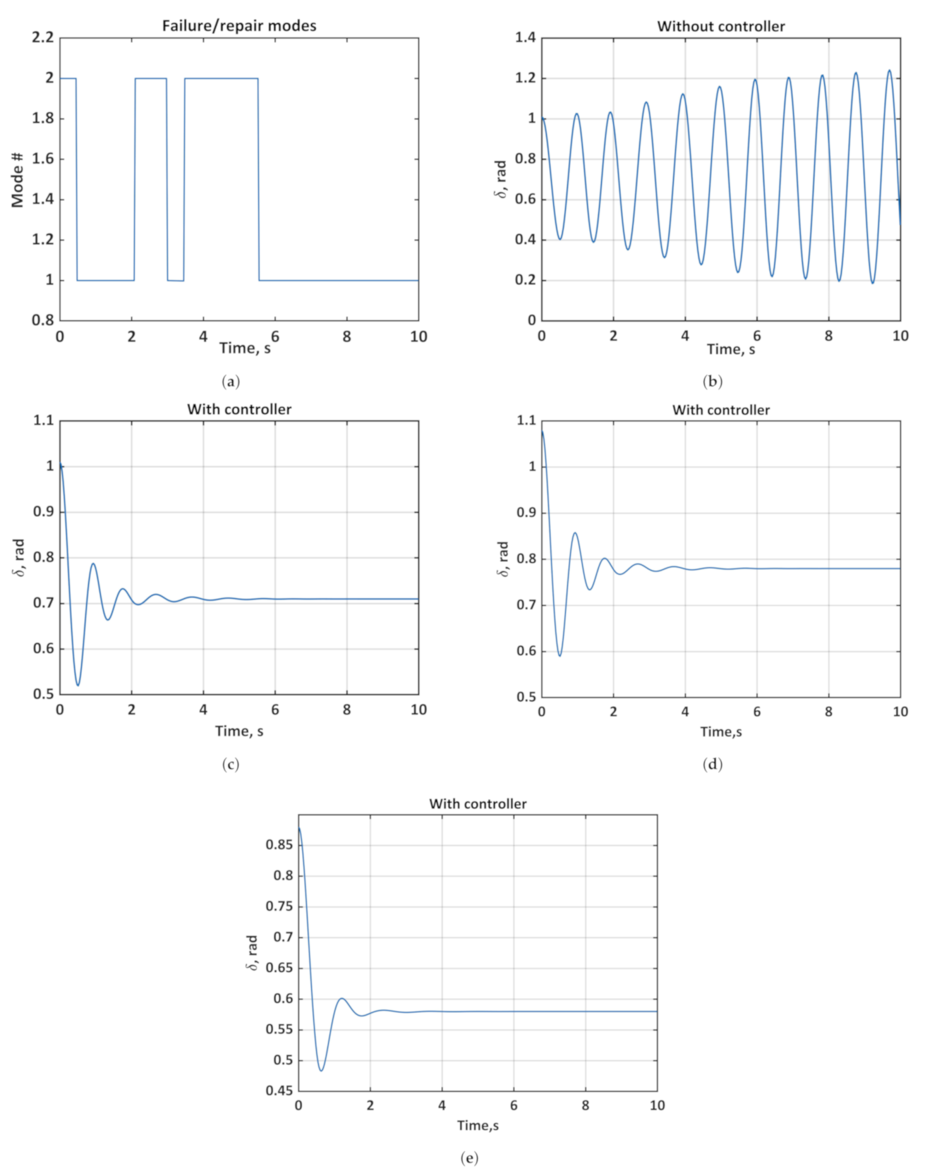
• For each of the two modes (failure/ repair), a stabilizer is designed to achieve the control target. The design avoids losing stability during the switching between the two controllers.
• This is the first time multi-controllers are designed based on the practical failure/ repair rates.

The rest of the paper is arranged as follows: Section 2 formulates the problem. The proposed methodology for addressing the problem is presented in Section 3. Section 4 demonstrates the simulation results. Finally, the paper is concluded in Section 5.

2. Problem Statements

For real matrices or vectors ${(}^{\prime })$ indicates transpose. For any matrix $P,P>0(<0)$ depicts that P is a symmetric positive (negative) definite matrix. To make things convenient regarding the notation of partitioned symmetric matrices, the symbol (*) is used that signifies each of its symmetric blocks generically. The set of non-negative integers is represented by N. The set of Markov chain states is $1,2,\dots N$. Given $N^2$ non-negative real numbers ${\pi }_{ij}$ satisfying ${\sum }_{j=1}^N{\pi }_{ij}=1,i=1,2,\dots ,N$. The symbol E{.} denotes mathematical expectation of {.}.

• For matrices $W_1,W_2$, the norm-bounded uncertainty $\Delta \left(k\right)<1$ can be eliminated using the fact: $(W_1·\Delta \left(k\right)·W_2+\ast )\le ϵW_1·W_1^{{}^{\prime }}+{ϵ}^{-1}{W}_2^{\prime }·W_2,ϵ\ge 0$.
• The nonlinear matrix equation can be linearized using the Schur complement: $W_1+W_3^{{}^{\prime }}·W_2^{-1}·W_3<0\leftrightarrow \left[\begin{array}{cc}{W}_1& \ast \\ W_3& -W_2\end{array}\right]<0$.

Figure 1 illustrates the block diagram of the studied system, where a single machine is connected to an infinite bus. The synchronous machine is equipped with a thyristor exciter. The study system is composed of two parallel transformers in series with two parallel lines. The infinite bus represents the Thévenin equivalent of a large network. The system reliability is evaluated at two extreme modes of operation: (1) no failure case, (2) stochastic failure/repair of one line and one transformer. The switching between the two modes results in a sudden topological change in the system and consequently jumps in system parameters. When the system is subject to a disturbance in both cases, designing a robust PSS to achieve useful oscillations damping within the desired settling time and damping ratio is required. In addition, the controller has to fulfil the control targets for different load changes.

The nonlinear model of the system is given by the following differential equations [1]:

$$\begin{array}{cc}\hfill & \dot{\delta }=w_0·\Delta w\hfill \\ \hfill & 2H\dot{\Delta w}=P_m-P_e=P_m-[E_q^{\prime }+(x_q-x_d^{\prime })I_d]I_q\hfill \\ \hfill & T_{d0}^{\prime }{\dot{E_q}}^{\prime }=E_f-[E_q^{\prime }+(x_d-x_d^{\prime })I_d]\hfill \\ \hfill & T_e\dot{E_f}=-E_f+K_e(V_{ref}-V_t+u)\hfill \end{array}$$

(1)

where $I_d,I_q,$ and $V_d$ are given by,

$$\begin{array}{cc}\hfill & I_d=(E_q^{\prime }-Vcos\delta )/(x_d^{\prime }+x_e)\hfill \\ \hfill & I_q=Vsin\delta /(x_q+x_e)\hfill \\ \hfill & V_t=\sqrt{{\left(I_q{x}_q\right)}^2+{(E_q^{\prime }-I_d{x}_d^{\prime })}^2}.\hfill \\ \hfill \end{array}$$

(2)

The above symbols are per unit (p.u.) unless otherwise stated. $\delta \left(t\right)$ is the power angle of the generator, in rad; $\omega \left(t\right)$ represents the relative speed of the the generator; ${\omega }_0$ is the synchronous machine speed; $P_m$ is the mechanical input power; $P_e\left(t\right)$ is the active electrical power; H is the inertia constant in seconds; $E_q^{\prime }\left(t\right)$ depicts the transient EMF in the quadrature axis; $E_q\left(t\right)$ is the EMF in the quadrature axis; $E_f\left(t\right)$ is the equivalent excitation EMF; $T_{d0}^{\prime }$ is the direct axis transient short circuit time constant, in seconds; $I_d\left(t\right)$ is the direct axis current; $I_q\left(t\right)$ is the quadrature axis current; $V_t\left(t\right)$ is the terminal voltage of the generator; $x_d$ is the direct axis reactance; $x_q$ is the quadrature axis reactance; $x_d^{\prime }$ is the direct axis transient reactance; and $x_q^{\prime }$ represents the quadrature axis transient reactance. In addition, $x_e=\frac{1}{2}(x_T+x_L)$ in no failure mode, $x_e=(x_T+x_L)$ in failure mode. Please note that $x_e,x_T,x_L$ are the external, transformer, and line reactances, respectively. Substituting (2) into (1), and linearize the resulting mathematical model for small oscillations around a nominal operating point to get:

$$\dot{x}=Ax+Bu$$

(3)

where $x=\Delta {[\delta ,\omega ,E_q^{\prime },E_{fd}]}^{\prime }$, $\delta =$ rotor angle in rad, $\omega =$ speed in per unit, $E_q^{\prime }=$ quadrature axis transient emf, and $E_{fd}=$ field voltage. The entries of the matrix A are functions of constants $k_1,k_2,$…$,k_6$. These constants are functions of the active and reactive load powers $(P,Q)$ injected at the infinite bus bar can be obtained numerically [1], or analytically [21].

$$A=\left[\begin{array}{cccc}0& w_0& 0& 0\\ \frac{-k_1}{M}& 0& \frac{-k_2}{M}& 0\\ \frac{-k_4}{T_{d0}^{\prime }}& 0& \frac{-1}{T}& \frac{1}{T_{d0}^{\prime }}\\ \frac{-k_5{k}_e}{T_e}& 0& \frac{-k_6{k}_e}{T_e}& \frac{-1}{T_e}\end{array}\right],B=\left[\begin{array}{c}0\\ 0\\ 0\\ \frac{k_e}{T_e}\end{array}\right]$$

(4)

where $M=2H$. The units of the parameters of SMIB data are considered in their per unit (p.u.) values unless otherwise stated. The data are given in

Table 1. Considered values of parameters for SMIB.

Elements	Parameters	Values
Synchronous machine	$x_d$	1.6
	$x_d^{\prime }$	0.32
	$x_q$	1.55
	${\omega }_o$	$2\pi \times 50$ rad/s
	$T_{d0}^{\prime }$	6 s
	H	5 s
Exciter + amplifier	$k_e$	25
	$T_e$	$0.05$ s
Transmission line + transformer	$x_e$	0.8
Nominal load (at infinite bus)	P	0.7
	Q	$0.3$

.

Please note that the apparent power for heavy, nominal, light loads is respectively: 1.1, 0.76, and 0.41. Appendix A presents the discrete-time SMIB model under load uncertainty (represented by a norm-bounded form) given in

Table 2. Different loading conditions.

Loading Condition	P (Per Unit)	Q (Per Unit)
Heavy	1	0.5
Nominal	0.7	0.3
Light	0.4	0.1

at modes 1, and 2.

The research goal is to design a robust PSS for adequate dynamic operational performance despite various loads and random topology changes. In practice, however, attaining satisfactory dynamic performance might not be possible via robust stability alone. The controller requires to damp oscillations caused by small disturbances within a short range of time (10–15 s) [22], i.e., the range of desired settling time ($t_s$) is 10–15 s. In the power system, the small oscillations occur within the range of 0.3–3 Hz; therefore, the system is discretized at a sampling time ($T_s)$ of 0.03 s, or at $10f_{max}$. In practice, damping of rotor swings is considered to be satisfactory if the damping ratio $\zeta \ge 0.15$ [22] (selected 0.3 in this paper). The common hatched area in Figure 2 satisfies both constraints of the desired damping ratio and settling time.

The power system dynamics under the stochastic failure/repair conditions of lines/ transformer, as shown in Figure 1, can be addresed by a discrete-time Markov jump linear system (MJLS) using the stochastic difference equation presented in (5).

$$x_{k+1}=A_i{x}_k+B_i{u}_k,x\left(0\right)=x_o,i=1,2,\dots ,N$$

(5)

where $x_kϵR^n,u_kϵR^m$ are the state and the control input at time k respectively. The state space matrices (5) depend on a Markov chain taking values in the finite set, $i=1,2,\dots ,N(N=2$ in our case) with the associated transition probability matrix $\pi ϵR^{N·N}$, whose elements are given by ${\pi }_{ij}$ and satisfying ${\sum }_{j=1}^N{\pi }_{ij}=1,$ for each $i=1,2,\dots ,N$. Figure 3 illustrates the state-transition probability of the studied system.

The problem is to develop a PSS,

$$u_k=F_i{x}_k$$

(6)

which stochastically stabilizes system (5). Please note that system (5) with $u_k=0$ for all $k=0,1,2,\dots$ is said to be stochastically stable if for all finite $x_0$ and the initial mode of transition probability, the following holds [23]:

$$E\{\sum _{k=0}^{\infty }\left|\right|x_k\left|\right|\}\le c\left|\right|x_0\left|\right|,c>0$$

(7)

where E is the expected value, and ‖(.)‖ is the norm of $(.)$. In addition to the above requirement, the PSS has to ensure an adequate dynamic performance, in terms of desired damping ratio, which is represented by a spiral in Figure 2 and settling time, which is represented by a circle in Figure 2, despite the system uncertainty (due to load changes) in both modes of operation. The closed-loop poles must stay in the hatched area shown in Figure 2, for achieving both constraints of damping ratio and settling time. This characteristic is regarded as D-stability in which the poles must stay within the desired D region for all possible uncertainties.

3. Proposed Methodology

The problem is solved in two steps: (1) modeling and evaluating Markov reliability of the SMIB study system for the extreme cases of most reliable and least reliable operations, (2) designing the PSS to fulfil regional pole placement under Markov Jumps between the two modes of operations. Please note that the power system reliability evaluation can be carried out by Monte Carlo simulation or by Markov process. The latter method is selected to avoid the enormous computation burden of the former [12].

3.1. Markov Reliability Evaluation

The SMIB study system is subject to random failure/repair of either line or transformer. This condition is modeled by Markov modelling. Assume that the failure rates and repair times for both transformers and transmission lines are as follows [8]:

Failure rate of a transformer (${\lambda }_T$) = 0.1 failure/year, repair time (${\Gamma }_T$) = 50 h.

Failure rate of a transmission line (${\lambda }_L$) = 5 failure/year, repair time (${\Gamma }_L$) = 15 h.

Reliability and unreliability values of any of the transformers and transmission lines can, then, be calculated as given in

Table 3. Calculation of parametes for reliability analysis.

Elements	Calculation
Transformers	Failure rate $\left({\lambda }_T\right)=0.1$ failure/year $=0.00001142$ failure/h
	Repair time $\left({\Gamma }_T\right)=50$ h
	Average annual outage time $={\lambda }_T·{\Gamma }_T$ $=0.000571$ $=$ Unreliability $\left(Q_T\right)$
	Reliability $\left(R_T\right)=1-{\lambda }_T·{\Gamma }_T$ $=0.999429$
	Repair rate $\left({\mu }_T\right)=1/{\Gamma }_T$ $=0.02$ repair/h
Transmission lines	Failure rate $\left({\lambda }_L\right)=5$ failure/year $=0.00057$ failure/h
	Repair time $\left({\Gamma }_L\right)=15$ h
	Average annual outage time $={\lambda }_L·{\Gamma }_L$ $=0.00855$ $=$ Unreliability $\left(Q_L\right)$
	Reliability $\left(R_L\right)=1-{\lambda }_T·{\Gamma }_T$ $=0.99145$
	Repair rate $\left({\mu }_L\right)=1/{\Gamma }_L$ $=0.067$ repair/h

.

Assuming full redundancy for both transformers as well as transmission lines for the study system shown in Figure 1, then, the system reliability $\left(R_{sys}\right)$ can be expressed as follows:

$$\begin{array}{cc}\hfill R_{sys}& =(R_T^2+2R_T·Q_T+Q_T^2)·(R_L^2+2R_L·Q_L+Q_L^2)\hfill \\ \hfill & =R_T^2{R}_L^2+2R_T^2{R}_L{Q}_L+R_T^2{Q}_L^2+2R_T{R}_L^2{Q}_T+4R_T{R}_L{Q}_T{Q}_L\hfill \\ \hfill & +2R_T{Q}_T{Q}_L^2+R_L^2{Q}_T^2+2R_L{Q}_T^2{Q}_L+Q_T^2{Q}_L^2\hfill \end{array}$$

(8)

where $R_T$ and $Q_T$ are the transformer reliability, and unreliability, respectively. $R_L$ and $Q_L$ are the line reliability and unreliability respectively. There will be 9-state Markov model for the above system. Among these nine states, only four are operable (success or up) states while the other five states are non-operable (failure or down) states where no output can be obtained from the system. The state probabilities for the operable (up) states can be calculated using (8) and are shown in

Table 4. State probabilities for the operable (UP) states.

UP States	Condition	State Probability
1	2T(U$)·2$L(U)	0.9818509
2	1T(U$)·1$L(U$)·1$T(D$)·1$L(D)	0.00001935
3	1T(U$)·2$L(U$)·1$T(D)	0.0011219
4	2T(U$)·1$L(U$)·1$L(D)	0.0169344

Where, U = Up, D = Down, T = transformer, L = transmission line.

.

Figure 4 illustrates the Markov model for the operable (UP) states. The highest and lowest state probabilities are of states 1 and 2 respectively as indicated in Table 4 and shown in Figure 4. Transition rates from the highest reliability state (Mode 1) to the lowest reliability state (Mode 2) are as follows:

Transition rate from Mode 2 to Mode 1

$=2({\lambda }_T+{\lambda }_L)$

$=2(0.00001142+0.00057)$

$=0.00116$$failure/h$

Transition rate from Mode 1 to Mode 2

$=2({\mu }_T+{\mu }_L)$

$=2(0.02+0.067)$

$=0.174$$repair/h$

The state-space diagram for the two states is shown in Figure 5.

From the above analysis, the transition probability matrix is presented in (9) and tabulated in

Table 5. Transition rate matrix.

System Reliability Condition	Mode 1	Mode 2
Maximum (Mode 1)	0.826	0.174
Minimum (Mode 2)	0.00116	0.99884

.

$$\pi =\left[\begin{array}{cc}0.826& 0.174\\ 0.00116& 0.99884\end{array}\right].$$

(9)

3.2. Regional Pole Placer Design for Power Systems under Markov Jumps

Achieving adequate dynamic behavior (under random failure /repair of lines/transformers in addition to load variations) requires placing the closed-loop poles in the hatched area of Figure 2. The solution to this problem is very complex mathematically. However, a simple solution can be obtained by approximating the spiral of the desired damping ratio by a circle as shown in Figure 6a. Based on this, a pole placer can be designed. Theorem 1 provides a sufficient condition in terms of LMIs to force the closed-loop poles to lie in the intersection of two circles which are the settling time and the damping ratio as shown in Figure 6b.

Theorem 1.

If there exists a feasible solution to the LMIs as presented in (10), the closed-loop poles of (3) will reside within the two circles of centre $q_1$ and radius $r_1$; and centre $q_2$ and radius $r_2$.

$$\begin{array}{cc}\hfill & X=X^{\prime }>0,{ϵ}_1>0,{ϵ}_2>0\hfill \\ \hfill & \left[\begin{array}{ccc}-r_1^{2}X& \ast & \ast \\ AX+BY+q_{1}X& -X+{ϵ}_{1}H{H}^{\prime }& \ast \\ EX& 0& -{ϵ}_{1}I\end{array}\right]<0\hfill \\ \hfill & \left[\begin{array}{ccc}-r_2^{2}X& \ast & \ast \\ AX+BY+q_{2}X& -X+{ϵ}_{2}H{H}^{\prime }& \ast \\ EX& 0& -{ϵ}_{2}I\end{array}\right]<0\hfill \\ \hfill \end{array}$$

(10)

Furthermore, the controller is given by $F=Y{X}^{-1}$.

Proof. 

See Appendix B. □

From the above, the following theorem can be stated.

Theorem 2.

There exists a state-feedback controller of the form (6) such that the closed-loop state equation of the system (5) is stochastically stable, under Markov modelling, and places the closed-loop poles in a desired region, despite load changes, if there remain a set of symmetric and positive-definite matrices $X=(X_1,\dots ,X_N)$ and a set of matrices $Y=(Y_1,\dots ,Y_N)$ such that the LMIs presented in (11) holds:

$$\begin{array}{cc}\hfill & X_i=X_i^{\prime }>0,{ϵ}_1>0,{ϵ}_2>0,{\rho }_i>0,\hfill \\ \hfill & \left[\begin{array}{ccc}-X_i& S_i& L_i\\ \ast & -Z+{\rho }_i\left[\begin{array}{c}0\\ H_i\end{array}\right]{\left[\begin{array}{c}0\\ H_i\end{array}\right]}^{\prime }\\ 0\\ \ast & \ast & -{\rho }_{i}I\end{array}\right]<0\hfill \\ \hfill & \left[\begin{array}{ccc}-r_1^2{X}_i& \ast & \ast \\ A_i{X}_i+B_i{Y}_i+q_1{X}_i& -X_i+{ϵ}_1{H}_i{H}_i^{\prime }& \ast \\ E_i{X}_i& 0& -{ϵ}_{1}I\end{array}\right]<0\hfill \\ \hfill & \left[\begin{array}{ccc}-r_2^2{X}_i& \ast & \ast \\ A_i{X}_i+B_i{Y}_i+q_2{X}_i& -X_i+{ϵ}_2{H}_i{H}_i^{\prime }& \ast \\ E_i{X}_i& 0& -{ϵ}_{2}I\end{array}\right]<0i=1,2,\dots ,N\hfill \\ \hfill \end{array}$$

(11)

where $S_i=[\sqrt{{\pi }_{i1}}(X_i{A}_i^{\prime }+Y_i^{\prime }{B}_i^{\prime })\dots \sqrt{{\pi }_{iN}}(X_i{A}_i^{\prime }+Y_i^{\prime }{B}_i^{\prime })],L_i=[\sqrt{{\pi }_{i1}}\left(X_i{E}_i^{\prime }\right)\dots \sqrt{{\pi }_{iN}}\left(X_i{E}_i^{\prime }\right)],$$Z=diag[X_1,\dots ,X_N]$. The gain of the controller is given by $F_i=Y_i{X}_i^{-1}$. Please note that the PSS’s design includes the transition rates as given in (11).

Proof. 

Combine the theorem in [18] with Theorem 2 in Appendix B. □

4. Simulation Results

Solving (11) provides the allows proposed PSS to stochastically stabilize the SMIB study system under Markov Jumps and achieve the desired settling time 12 s, and damping ratio 0.3 (the closed-loop poles must be placed in the intersection between two circles, $q_1=0,r_1=0.99,$ and $q_2=-0.31,r_2=0.6.$). The set of equations (11) are solved using the Matlab LMI toolbox, Yalmip interface, and SEDUMI solver. The resulting controllers are:

$F_1^{\ast }=\left[\begin{array}{cccc}-0.3033& 425.5083& -4.4442& -0.0288\end{array}\right]$

$F_2^{\ast }=\left[\begin{array}{cccc}-1.6863& 251.9006& -2.5022& -0.0240\end{array}\right]$

The closed-loop poles using the proposed PSS for different load changes and either failure/repair mode of operation are given in Figure 7a,b. It is evident that the poles lie inside the desired region satisfying the required settling time and damping ratio. However, if the designer feels that the obtained controllers $F_1^{\ast },F_2^{\ast }$ have high gains which may result in violating the practical limits of the control signal, he can relax the damping ratio to a lower value. In this case, the obtained controllers with lower gains are:

$F_1=\left[\begin{array}{cccc}-0.9296& 40.6432& -0.8580& -0.0196\end{array}\right]$

$F_2=\left[\begin{array}{cccc}-0.6547& 13.8107& -0.0092& -0.0177\end{array}\right]$

Consider the SMIB system at heavy load (worst case) is subject to a cleared fault at $t=0$ s, which causes 0.3 rad perturbation in the torque angle. This is an unstable system without the controller. Figure 8a demonstrates random failure/repair modes, whereas Figure 8b,c illustrates the performance of the system without the controller and with the proposed controller respectively under nominal load condition. In Figure 8d,e, response of the system in different load (heavy and light) conditions have been shown with the proposed controller. According to the simulation results, the open-loop response of the system without controller shows instability under failure/repair modes. Conversely, from the closed-loop response, it can be clearly depicted that, the proposed controller provides excellent performance under failure/repair modes as well as in different load conditions.

Please note that at the least reliable contingency case, the system is heavily loaded and the stability margin become less. Therefore, the closed loop poles becomes nearer to the boundary of the desired damping curve.

5. Conclusions

This paper presented design and performance analysis of regional pole placer-based control for power system applications under random uncertainties. The transition probability matrix of such uncertainties, such as random failure/repair of lines/transformers SMIB system is derived to describe the Markov reliability. Power system stabilization under Markov Jumps is considered. In addition to stabilization, the proposed controller achieves adequate dynamic performance in terms of the desired settling time and damping ratio against load changes. A sufficient condition in the LMI platform is derived. Simulations are performed under varying load conditions to prove the efficacy of the proposed controller. The designed controller has shown satisfactory dynamic performance under random failure/repair conditions with varying load changes. In future, practical implementation with experimental setup will be considered to verify the simulated results.

References

1. Machowski, J.; Lubosny, Z.; Bialek, J.W.; Bumby, J.R. Power System Dynamics Stability and Control, 3rd ed.; John Wiley & Sons Ltd.: Hoboken, NJ, USA, 2020. [Google Scholar]
2. Farahan, M.; Ganjefar, S. Intelligent power system stabilizer design using adaptive fuzzy sliding mode controller. Neurocomputing 2017, 226, 135–144. [Google Scholar] [CrossRef]
3. Sarita, K.; Kumar, S.; Vardhan, A.S.S.; Elavarasan, R.M.; Saket, R.K.; Shafiullah, G.M.; Hossain, E. Power enhancement with grid stabilization of renewable energy-based generation system using UPQC-FLC-EVA technique. IEEE Access 2020, 8, 207443–207464. [Google Scholar] [CrossRef]
4. Salgotra, A.; Pan, S. Model based PI power system stabilizer design for damping low frequency oscillations in power systems. ISA Trans. 2018, 76, 110–121. [Google Scholar] [CrossRef] [PubMed]
5. Soliman, H.M.; Ghommam, J.R. Reliable Control of Power Systems; Chapter in the book Diagnosis, Fault Detection & Tolerant Control; Springer: Berlin/Heidelberg, Germany, March 2020. [Google Scholar]
6. Hossain, E.; Hossain, J.; Un-Noor, F. Utility grid: Present challenges and their potential solutions. IEEE Access 2018, 6, 60294–60317. [Google Scholar] [CrossRef]
7. Hu, W.; Liang, J.; Jin, Y.; Wu, F. Model of Power System Stabilizer Adapting to Multi-Operating Conditions of Local Power Grid and Parameter Tuning. Sustainability 2018, 10, 2089. [Google Scholar] [CrossRef] [Green Version]
8. Konara, A.I.; Annakkage, U.D. Robust Power System Stabilizer Design Using Eigenstructure Assignment. IEEE Trans. Power Syst. 2016, 31, 1845–1853. [Google Scholar] [CrossRef]
9. Ahshan, R.; Iqbal, M.T.; Mann, G.K.; Quaicoe, J.E. Microgrid reliability evaluation considering the intermittency effect of renewable energy sources. Int. J. Smart Grid Clean Energy 2017, 6, 252–268. [Google Scholar] [CrossRef]
10. Urgun, D.; Singh, C. A hybrid monte carlo simulation and multi label classification method for composite system reliability evaluation. IEEE Trans. Power Syst. 2018, 34, 908–917. [Google Scholar] [CrossRef]
11. Huda, A.N.; Živanović, R. Accelerated distribution systems reliability evaluation by multilevel Monte Carlo simulation: Implementation of two discretisation schemes. IET Gener. Transm. Distrib. 2017, 11, 3397–3405. [Google Scholar] [CrossRef]
12. Billinton, R.; Allan, R.N. Reliability Evaluation of Engineering Systems: Concepts and Techniques, 2nd ed.; Springer Science and Business Media: New York, NY, USA, 1992. [Google Scholar]
13. Elmakias, D. New Computational Methods in Power System Reliability; Springer: Berlin/Heidelberg, Germany, 2008. [Google Scholar]
14. Hou, K.; Jia, H.; Xu, X.; Liu, Z.; Jiang, Y. A continuous time Markov chain based sequential analytical approach for composite power system reliability assessment. IEEE Trans. Power Syst. 2015, 31, 738–748. [Google Scholar] [CrossRef]
15. Lisnianski, A.; Elmakias, D.; Laredo, D.; Haim, H.B. A multi-state Markov model for a short-term reliability analysis of a power generating unit. Reliab. Eng. Syst. Saf. 2012, 98, 1–6. [Google Scholar] [CrossRef]
16. Soliman, H.; Shafiq, M. Robust stabilisation of power systems with random abrupt changes. IET Gener. Transm. Distrib. 2015, 9, 2159–2166. [Google Scholar] [CrossRef]
17. Ray, P.K.; Paital, S.R.; Mohanty, A.; Eddy, F.Y.; Gooi, H.B. A robust power system stabilizer for enhancement of stability in power system using adaptive fuzzy sliding mode control. Appl. Soft Comput. 2018, 73, 471–481. [Google Scholar] [CrossRef]
18. Ugrinovskii, V.; Pota, H.R. Decentralized control of power systems via robust control of uncertain Markov jump parameter systems. Int. J. Control 2005, 78, 662–677. [Google Scholar] [CrossRef]
19. Ma, J.; Wang, S.; Qiu, Y.; Li, Y.; Wang, Z.; Thorp, J.S. Angle Stability Analysis of Power System With Multiple Operating Conditions Considering Cascading Failure. IEEE Trans. Power Syst. 2017, 32, 873–882. [Google Scholar] [CrossRef]
20. Wu, W.; Wen, F.; Xue, Y.; Zhao, X.; Hu, R. A Markov chain based model for forecasting power system cascading failures. Dianli Xitong Zidonghua (Autom. Electr. Power Syst.) 2013, 37, 29–37. [Google Scholar]
21. Soliman, H.M.; Elshafei, A.L.; Shaltout, A.A.; Morsi, M.F. Robust power system stabiliser. IEE Proc. Gener. Transm. Distrib. 2000, 147, 285–291. [Google Scholar] [CrossRef]
22. Passrba, J. Analysis and Control of Power System Oscillations; Technical Brochure 111. 1996. Available online: https://e-cigre.org/publication/111-analysis-and-control-of-power-system-oscillations (accessed on 2 April 2021).
23. Benzaouia, A. Saturated Switching Systems; Springer: London, UK, 2012. [Google Scholar]
24. Haddad, W.M.; Bernstein, D.S. Controller design with regional pole constraints. IEEE Trans. Autom. Control 1992, 37, 54–69. [Google Scholar] [CrossRef]
Figure 1. Block diagram of the studied system, single machine infinite bus (SMIB) under failure/repair modes.
Energies 14 01989 g001
Figure 2. Closed-loop poles of the system, where the hatched area indicates the desired region (not to scale).
Energies 14 01989 g002
Figure 3. Graphical illustration of state-transition probability.
Energies 14 01989 g003
Figure 4. Four-operable (successful or UP) states Markov model.
Energies 14 01989 g004
Figure 5. State-space diagram of the highest and lowest reliability modes.
Energies 14 01989 g005
Figure 6. (a) ζ -approximation, and (b) expected region of poles (the hatched area) of the proposed system (not to scale).
Energies 14 01989 g006
Figure 7. Closed-loop poles for different load changes, (a) mode 1 (maximum reliability) (b) mode 2 (minimum reliability).
Energies 14 01989 g007
Figure 8. SMIB system response subject to random failure/repair modes under varying load conditions, such as (a) Random failure/repair modes (b) Open-loop response (c) Closed-loop response at the nominal load (d) Closed-loop response at the heavy load (e) Closed-loop response at the light load.
Energies 14 01989 g008