Model Predictive Control with Adaptive Building Model for Heating Using the Hybrid Air-Conditioning System in a Railway Station

Abstract

A model predictive control (MPC) system with an adaptive building model based on thermal-electrical analogy for the hybrid air conditioning system using the radiant floor and all-air system for heating is proposed in this paper to solve the heating supply control difficulties of the railway station on Tibetan Plateau. The MPC controller applies an off-line method of updating the building model to improve the accuracy of predicting indoor conditions. The control performance of the adaptive MPC is compared with the proportional-integral-derivative (PID) control, as well as an MPC without adaptive model through simulation constructed based on a TRNSYS-MATLAB co-simulation testbed. The results show that the implementation of the adaptive MPC can improve indoor thermal comfort and reduce 22.2% energy consumption compared to the PID control. Compared to the MPC without adaptive model, the adaptive MPC achieves fewer violations of constraints and reduces energy consumption by 11.5% through periodic model updating. This study focuses on the design of a control system to maintain indoor thermal comfort and improve system efficiency. The proposed method could also be applied in other public buildings.

1. Introduction

With the rapid development of the economy and urbanization, the total energy consumption of buildings has increased sharply. In recent years, with the growth of the scale of public buildings and the increase of terminal energy demand (such as air conditioning, equipment, lighting, etc.), public buildings account for 33% of the total building energy consumption, which is the largest proportion of all types of buildings [1]. As a common public building, railway passenger station has the characteristics of large space, large window-wall ratio and a great variation of personnel flow, causing the increase of energy consumption of HVAC system, which accounts for 60–80% of the total energy consumption [2]. In addition, the control and operation of HVAC system have a significant impact on the energy consumption of buildings [3]. Therefore, the design and optimization of the control system becomes crucial for energy saving.

At present, the serial control based on terminal feedback is mostly used in railway passenger station. Due to the large control area, complex air conditioning system and thermal inertia of the building, the above traditional control mode such as PID control normally has serious hysteresis, which leads to the problem of overheating or overcooling in the zone. In recent years, the research and application of the MPC approach has generally expanding owing to its many advantages, such as its anticipatory control actions, the ability to handle time-varying system dynamics and the integration of energy conservation strategies in control optimizer, etc. [4]. The MPC employs control-oriented building models to predict future states of the system and outputs a control value that are calculated by the controller to minimize a default cost function over the prediction horizon under constraints and disturbances. The optimal solution of the optimization problem is given by a sequence of optimal control actions, but only the first control action is applied to the system, following the policy of receding horizon control [5]. Moreover, the MPC is superior to other control method in temperature control and energy saving due to its advanced optimal control algorithm realized by the appropriate predictive model, receding horizon optimization and timely feedback correction [6].

Applying MPC to air conditioning system has gained increasing attention in recent researches. Hu et al. [7] implemented MPC systems for a radiant floor system in the living room of a residential apartment, which improved thermal comfort and reduced 2–19% of daily electricity costs. Joe et al. [8] developed an MPC controller for hydronic radiant floor systems in office buildings, energy savings of 34% were achieved in the cooling season and 16% in the heating season compared to baseline feedback control. Yang et al. [9] reported a test cell with the fan coil unit to cooling which applied the MPC controller achieved 6–19% energy savings as compared to the conventional on/off control. Afram et al. [10] designed an MPC controller based on supervisory for the residential HVAC systems which applied multi-zone AHU in summer and radiant floor heating systems in winter, achieving up to 50% cost savings. An exhaustive review [4] showed that the MPC controller has better performance in terms of energy savings, peak load shifting capability and robustness to dynamic disturbances, etc., compared to other control methods. Although previous researches developed MPC approaches in different air conditioning systems, the hybrid air conditioning system applied in single cooling or heating season has not been investigated. In addition, most of the MPC applications studied before were small zones like residential buildings [10], office buildings [8,11], computer room [12] and test room [9], etc. Few studies have applied MPC for large space public buildings such as railway passenger stations [13,14]. This study will provide a reference for the control strategy of large space hybrid heating system.

The accuracy of the building model to predict the future building state is crucial for the MPC controller. Generally, the black-box model [15,16,17] and the grey-box model [7,8,10] are applied to develop the building model. Compared to the black-box model, the grey-box model has better generalization capabilities based on the prior knowledge of thermal features and valid measured data [18,19]. Moreover, compared with other black or grey models, lumped RC (thermal resistance–thermal capacity) networks are more precise and robust because their parameters have distinct physical meanings and the models need less data than data-driven models [20]. Therefore, the lumped RC networks are often utilized for establishing reduced-order thermal network models to describe the heat transfers between network nodes to study the heat transfer of different types of heating systems [21,22,23,24].

In this study, an MPC system is developed using an RC-model-based building dynamic model to control the hybrid air conditioning system to achieve efficient energy use and maintain human thermal comfort. The grey-box model identification process depending on the measurement data associated with the building’s physical characteristics. Because the building physical characteristics affected by external disturbances like weather or internal heat source are not invariable, the model needs a continuous update to capture variations of characteristics [25,26]. Consequently, a new method to update the building model relying on the collected data applied to the MPC system is presented in this paper. The innovation spots of the work lie in: (1) develops the MPC system in the large space to solve overheating or overcooling of indoor environment problem caused by the poor control system of Tibetan Plateau heating. (2) presents an adaptive MPC method for the hybrid air conditioning system (i.e., the radiant floor and all-air system for heating) based on data-driven updated building models.

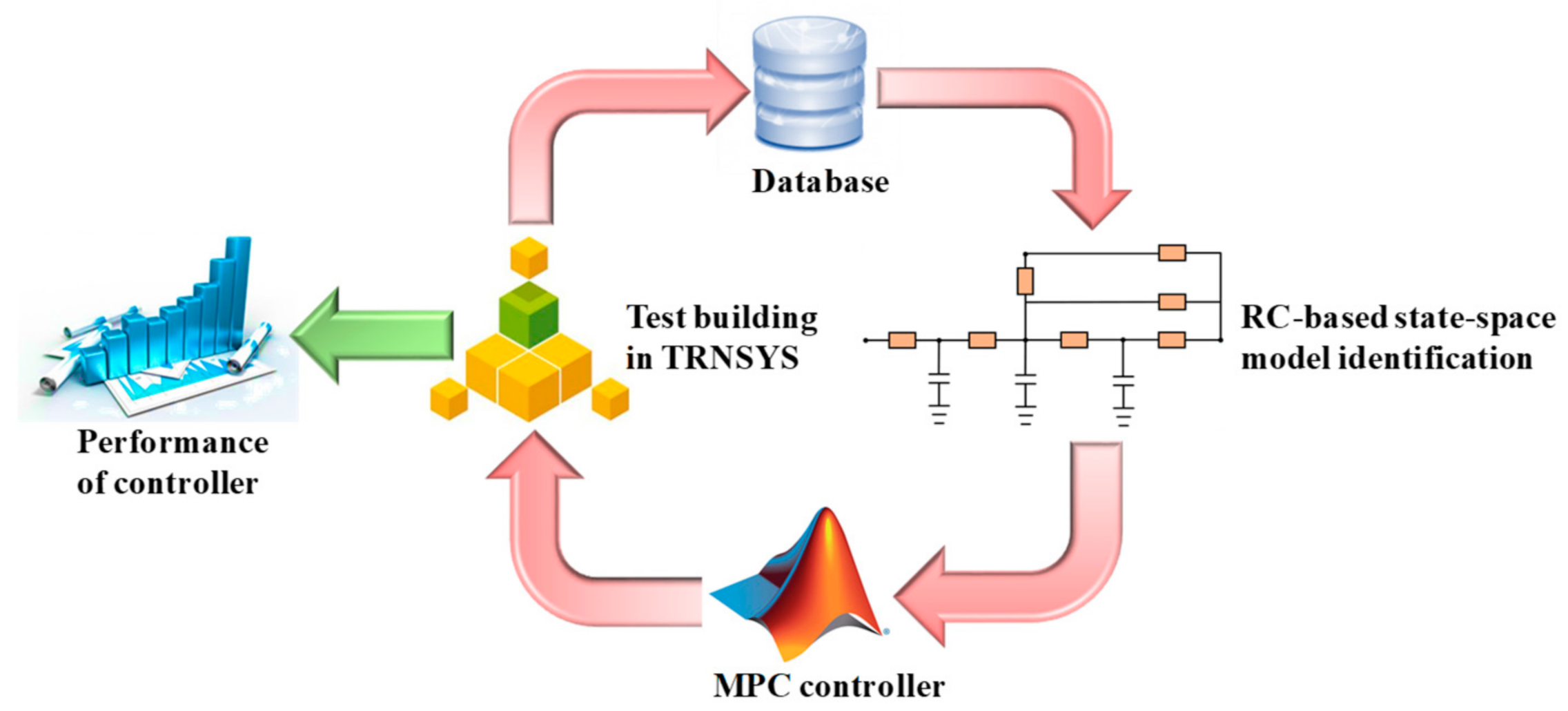
2. The Overview of Research Methodology

Until the building is completed, the actual operation data is very difficult to obtain. Therefore, an accurate building model needs to be established using simulation software such as TRNSYS, EnergyPlus at first. The state space model is the most commonly used in selection of the model in MPC nowadays. In fact, theoretical advances of MPC field were made focusing mainly on the state space prediction equations [27]. Hence, in this paper, the state space equations are adopted to organize system dynamics and the simulated data are used to identify the parameters in control equations. Figure 1 gives an overview of the methodology adopted in this research. Firstly, original building operation data is collected to construct and train an initial state space model based on the RC model of building by TRNSYS. The initial model is then applied to formulate an initial MPC controller to perform the real-time control effect of the building and a new set of building operation data will be obtained afterward. The new data set is stored and fed back at each control interval for the renovation of the building model periodically at a time interval and a new MPC controller is formulated termly applying the updated model to control the system during the next model adaption cycle. At last, the control performance of the adaptive MPC is evaluated by comparing it to the PID control and the MPC without adaptive modeling designed by initial operation data. In this research, the proposed MPC controller with an adaptive building model is developed in a waiting hall of a high-speed railway passenger station, as presented in Section 4.

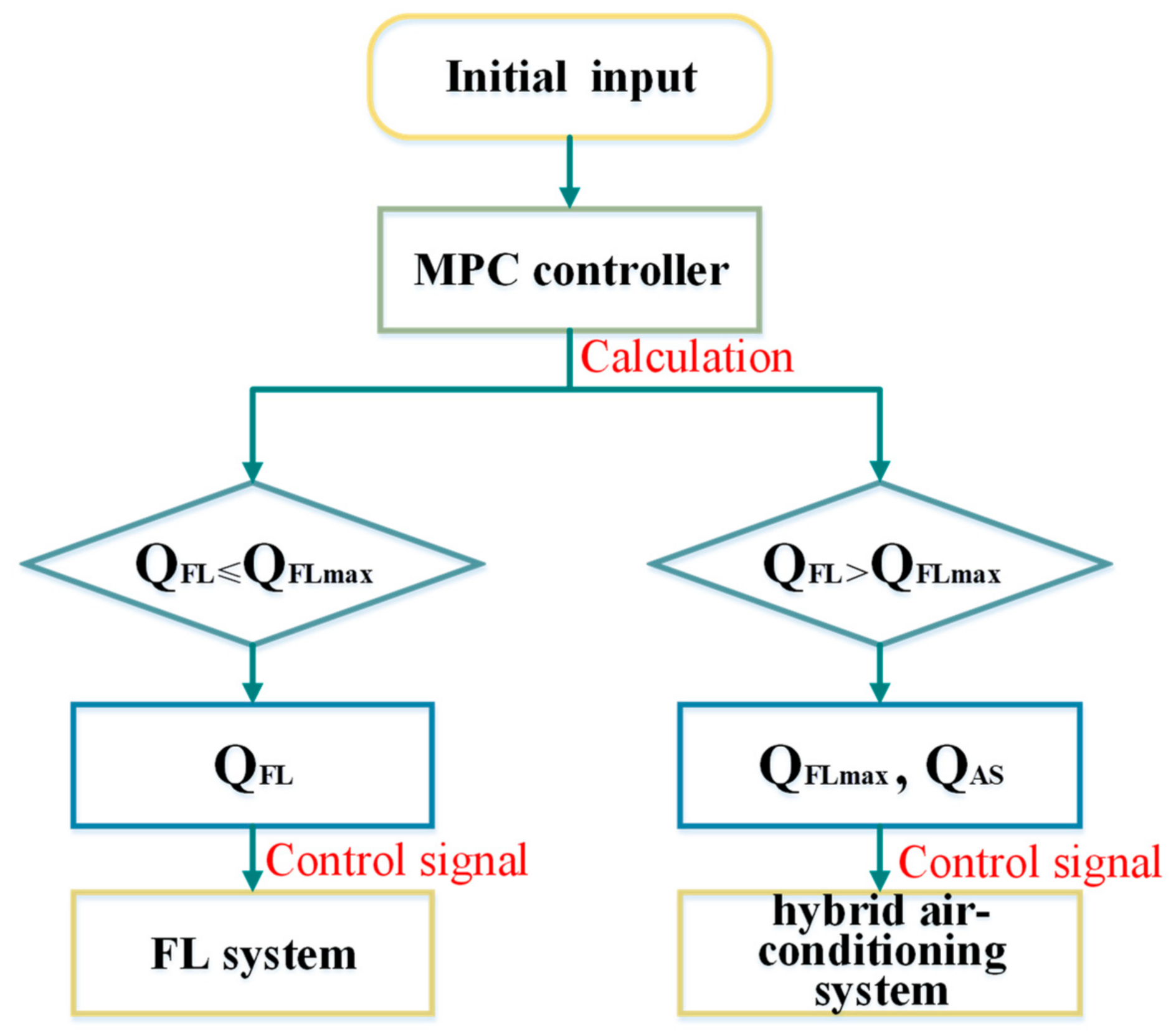
3. MPC Controller Design

Figure 2 shows an overall framework of the proposed MPC system implemented in the building. The state space model is initialized using zone operation data measured by regulating the water supply flow of the hybrid air conditioning system in TRNSYS. According to the state space model, cost function, constraints, real-time state variables and disturbances, the optimal control signal calculated by the optimizer will be applied to the air conditioning system. At the same time, the measured data of zone conditions is stored to update state space model weekly. The model adaption time interval is one week, which is illustrated in Section 3.5. Radiant heating and cooling systems are identified as an effective pathway to achieve energy-saving and improve indoor thermal comfort compared to all-air systems [28,29]. Therefore, the design principle of the controller is to give priority to radiant floor heating as shown in Figure 3. When the predicted heating amount of radiant floor Q_FL reaches the maximum heat transfer of floor Q_FLmax, the all-air system is turned on to supplement the insufficient heating amount Q_AS. A validation calculation analysis, meanwhile, is presented in Section 5.1 to demonstrate that the radiation floor heating system is more energy efficient than the all-air system in separate heating. The specific design of the controller will be described in detail below.

3.1. Dynamic Thermal Model for Building

The design of MPC controller is based on mathematical modeling to solve the optimization problem. An adequately accurate model can obtain valid predictions of the relevant control variables and the model must be simplified for the controller to be computationally tractable and numerically stable. With the RC method, parameters of the building dimensions and materials can be incorporated into a high-order model while maintaining the thermal passivity of the integral structure. In the RC-network model, each wall is characterized by a system of resistances and capacitances, each airspace is characterized by a single capacitance while the value of resistance and capacitance parameters are determined by building materials and dimensions. Meanwhile, temperatures and heat flows are identified as voltages and currents, respectively [23]. Further, the structure of the network depends on the specific zone being modeled. The following subsections describe the RC model for each subsystem.

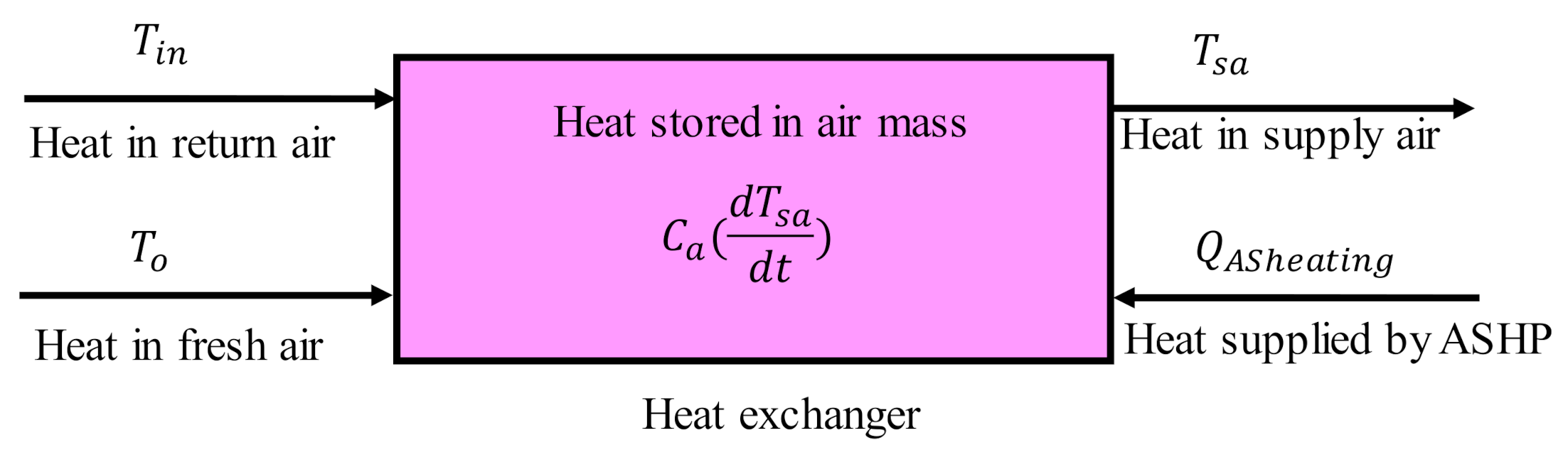
3.1.1. Model of All-Air System

The air–water surface heat exchanger constitutes the modeling of all air-system. As shown in Figure 4, the heat exchanger energy balance is related to fresh air (T_o), return air (T_in), supply air (T_sa) and heat supplied by heat source (Q_AS) [22,24]. To facilitate the establishment and solution of the model, it is assumed that the air was an ideal gas and the variation of fluid density and heat capacity were ignored.

The supply air temperature T_sa is calculated as Equation (1).

$$C_a\frac{{dT}_{sa}}{dt} = \frac{T_{in}-T_{sa}}{R_{\mathit{in},\mathit{sa}}}+\frac{T_o-T_{sa}}{R_{o,\mathit{sa}}}+Q_{AS}$$

(1)

where T_in, T_o, C_a, R_in,sa, R_o,sa are the temperature of the return air (indoor air), the temperature of fresh air (outdoor air), thermal capacitance of heat exchanger, thermal resistance between return air and supply air and thermal resistance between fresh air and supply air, respectively.

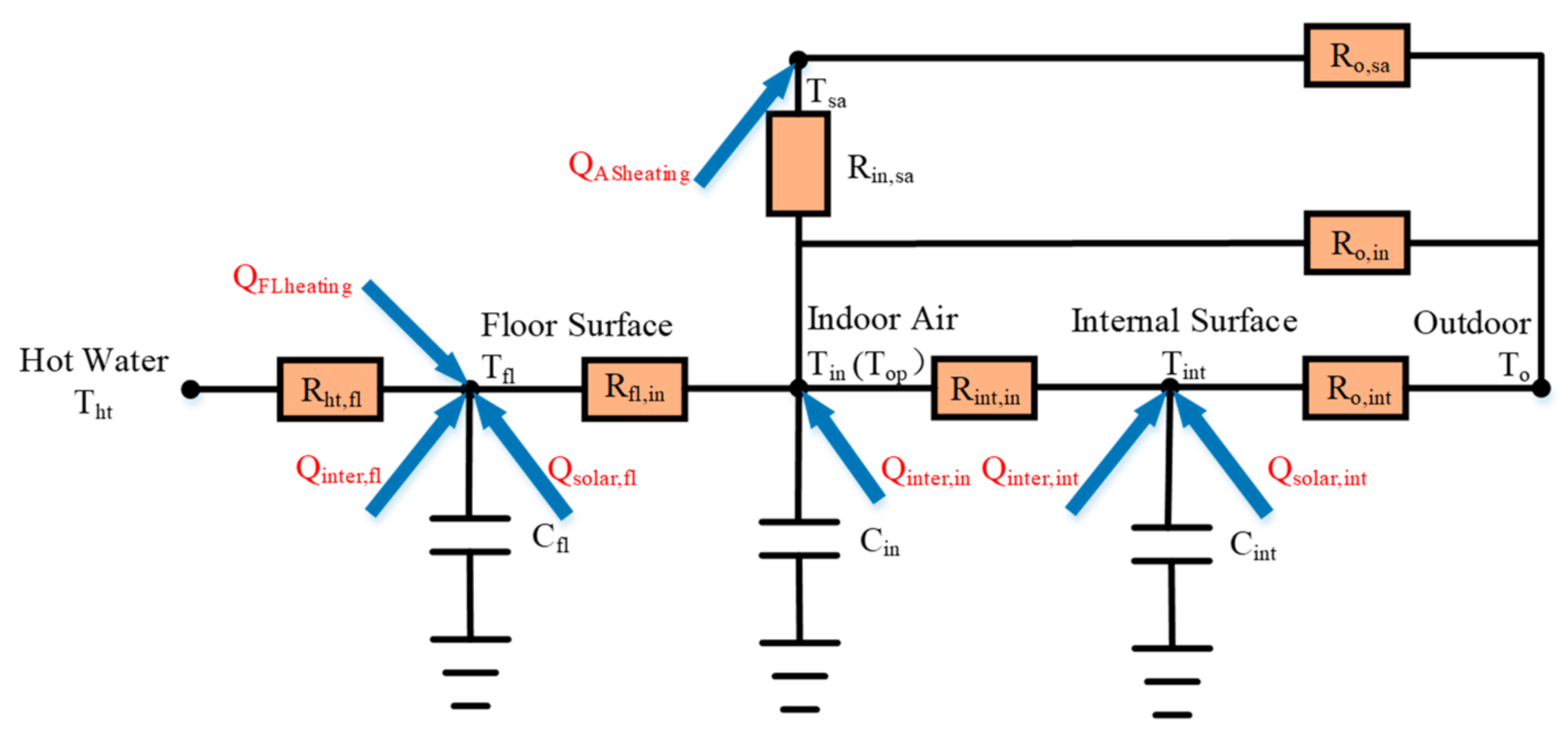
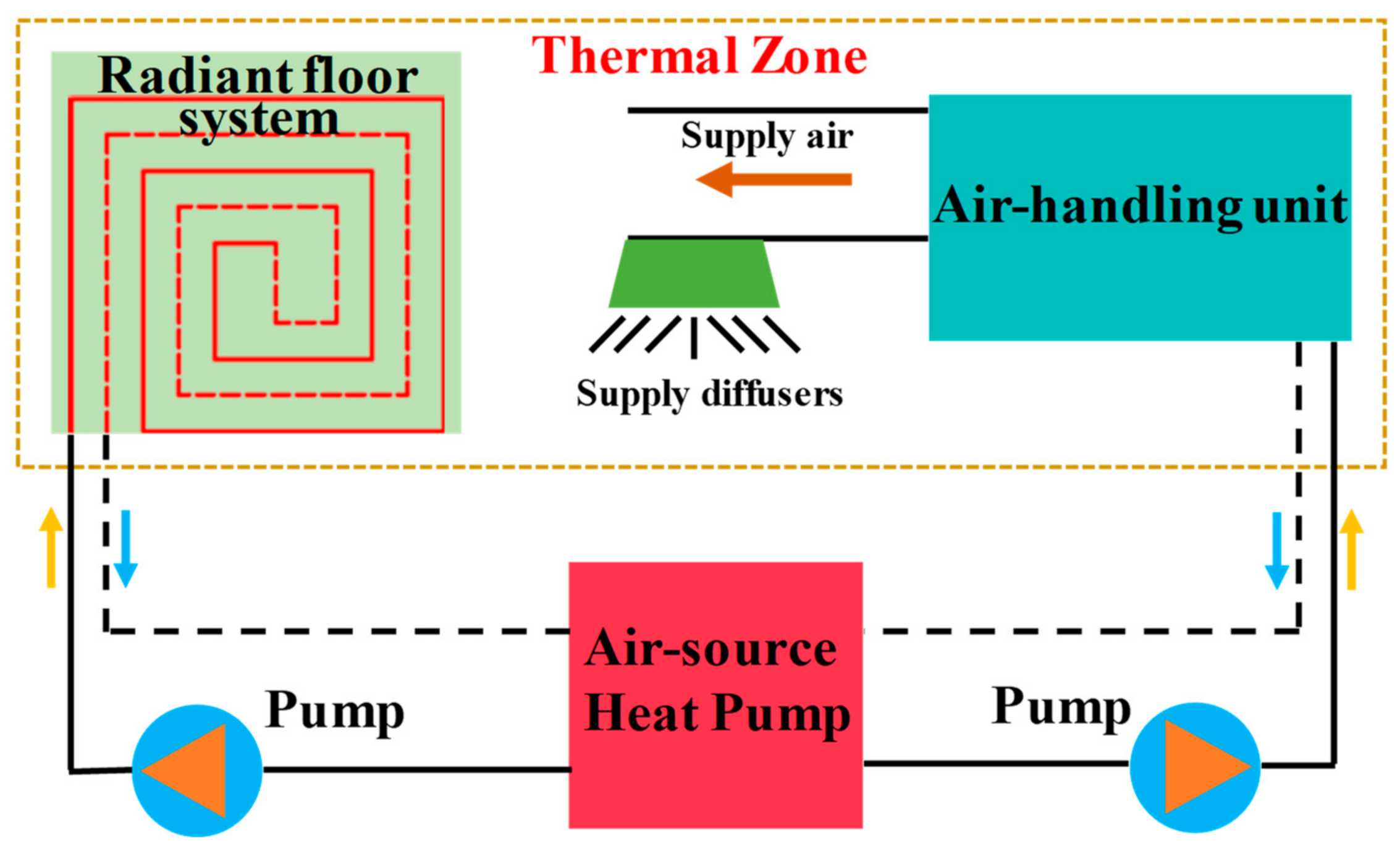
3.1.2. Model of Zone with the Hybrid Air Conditioning System

As presented in Figure 5, the heat transfer process of the integrated air conditioning system model has been constructed for both radiative and convective heating systems. To facilitate the design of the controller, the monitoring parameters of the system should be as few as possible. Therefore, it is considered to establish a direct relationship between indoor parameters and external disturbances. For example, the inner surface of wall temperature (T_int) is relevant to the outer surface of wall temperature which is affected by the ambient temperature (T_o) and incident solar radiation (Q_solar). However, it is difficult to measure the temperature of the outer surface of wall and the model of the outer surface of wall can be omitted, then the relationship between inner surface of wall temperature, ambient temperature and incident solar radiation can be established directly. This reduced-order method is testified to be more fast and precise in parameter identification as shown in Section 4.10. The energy balance equations for inner surface of wall, indoor air temperature and operative temperature can be categorized in Equations (2)–(4), respectively. R and C denote the overall heat resistance and capacitance; subscripts int, sa, in and op represent inner surface of wall, supply air, indoor air and variables related to operative temperature. A three-node model (hot water node, interior node and surface node) is generally utilized to simulate the thermal mass of floor heating [21]. On account of the temperature of the pipe network is difficult to measure, the relationship between heating quantity, the temperature of supply water and floor temperature are constructed as Equation (5). The values of thermal capacity and thermal resistance of floor heating are determined by pipe plane spacing, filling layer thickness, filling layer material, etc. [20]. Thus, a constant value of thermal resistance (R_ht,fl) can be used to represent the relationship between the hot water temperature (T_ht) and the floor surface temperature (T_fl). Q_FL represents the heat transferred from the heating system to the pipe network.

$$C_{\mathit{int}}\frac{{\mathit{dT}}_{\mathit{int}}}{\mathit{dt}} = \frac{T_{\mathit{sa}}-T_{\mathit{int}}}{R_{\mathit{int},\mathit{sa}}} + \frac{T_{\mathit{in}}-T_{\mathit{int}}}{R_{\mathit{int},\mathit{in}}} + \frac{T_{\mathit{op}}-T_{\mathit{int}}}{R_{\mathit{int},\mathit{op}}} + \frac{T_{\mathit{fl}}-T_{\mathit{int}}}{R_{\mathit{fl},\mathit{int}}} + \frac{T_o-T_{\mathit{int}}}{R_{o,\mathit{int}}} + Q_{\mathit{solar},\mathit{int}} + Q_{\mathit{inter},\mathit{int}}$$

(2)

$$C_{\mathit{in}}\frac{{\mathit{dT}}_{\mathit{in}}}{\mathit{dt}} = \frac{T_{\mathit{sa}}-T_{\mathit{in}}}{R_{\mathit{in},\mathit{sa}}} + \frac{T_{\mathit{int}}-T_{\mathit{in}}}{R_{\mathit{in},\mathit{int}}} + \frac{T_{\mathit{op}}-T_{\mathit{in}}}{R_{\mathit{in},\mathit{op}}} + \frac{T_{\mathit{fl}}-T_{\mathit{in}}}{R_{\mathit{in},\mathit{fl}}} + \frac{T_o-T_{\mathit{in}}}{R_{\mathit{in},o}} + Q_{\mathit{inter},\mathit{in}}$$

(3)

$$C_{\mathit{op}}\frac{{\mathit{dT}}_{\mathit{op}}}{\mathit{dt}} = \frac{T_{\mathit{sa}}-T_{\mathit{op}}}{R_{\mathit{op},\mathit{sa}}} + \frac{T_{\mathit{int}}-T_{\mathit{op}}}{R_{\mathit{op},\mathit{int}}} + \frac{T_{\mathit{in}}-T_{\mathit{op}}}{R_{\mathit{op},\mathit{in}}} + \frac{T_{\mathit{fl}}-T_{\mathit{op}}}{R_{\mathit{op},\mathit{fl}}} + \frac{T_o-T_{\mathit{op}}}{R_{\mathit{op},o}} + Q_{\mathit{inter},\mathit{op}}$$

(4)

$$C_{\mathit{fl}}\frac{{\mathit{dT}}_{\mathit{fl}}}{\mathit{dt}} = \frac{T_{\mathit{sa}}-T_{\mathit{fl}}}{R_{\mathit{fl},\mathit{sa}}} + \frac{T_{\mathit{int}}-T_{\mathit{fl}}}{R_{\mathit{fl},\mathit{int}}} + \frac{T_{\mathit{in}}-T_{\mathit{fl}}}{R_{\mathit{fl},\mathit{in}}} + \frac{T_{\mathit{op}}-T_{\mathit{fl}}}{R_{\mathit{fl},\mathit{op}}} + \frac{T_{\mathit{ht}}-T_{\mathit{fl}}}{R_{\mathit{fl},\mathit{ht}}} + Q_{\mathit{solar},\mathit{fl}} + Q_{\mathit{inter},\mathit{fl}} + Q_{\mathit{FLheating}}$$

(5)

Equations (2)–(5) represent that heat exchange occurs between indoor air, internal surface of envelopes, supply air and outdoor air. In addition, building interior parameters are affected by incident solar radiation and internal heat sources. Equations (6)–(11) represent the effect of internal heat gains and incident solar radiation on node temperature. Q_inter denotes the internal heat gains, including occupants, lights and equipment. It has an effect on the temperature of internal surfaces (Q_inter,int), indoor air (Q_inter,in), floor (Q_inter,fl) and operative temperature (Q_inter,op). Q_solar denotes the heat gains from incident solar radiation, involving the effect on internal surface (Q_solar,int) and floor (Q_solar,fl). F denotes the conversion coefficients for the heat gains, which are also identified together with RC models; I_solar denotes the global incident solar radiation; A denotes the geometric area. In addition, the internal heat sources from occupants, lights and equipment are supposed to be absorbed immediately [7].

$$Q_{\mathit{inter},\mathit{int}} = F_{\mathit{inter},\mathit{int}}{Q}_{\mathit{inter}}$$

(6)

$$Q_{\mathit{inter},\mathit{in}} = F_{\mathit{inter},\mathit{in}}{Q}_{\mathit{inter}}$$

(7)

$$Q_{\mathit{inter},\mathit{op}} = F_{\mathit{inter},\mathit{op}}{Q}_{\mathit{inter}}$$

(8)

$$Q_{\mathit{inter},\mathit{fl}} = F_{\mathit{inter},\mathit{fl}}{Q}_{\mathit{inter}}$$

(9)

$$Q_{\mathit{solar},\mathit{int}} = F_{\mathit{solar},\mathit{int}}{A}_{\mathit{int}}{I}_{\mathit{solar}}$$

(10)

$$Q_{\mathit{solar},\mathit{fl}} = F_{\mathit{solar},\mathit{fl}}{A}_{\mathit{win}}{I}_{\mathit{solar}}$$

(11)

3.2. Model Transformation

Based on the above RC dynamic thermal model, a continuous-time, linear state space model can be described as Equations (12) and (13).

$$\frac{\mathit{\partial }x\left(t\right)}{\partial t} = A_{c}x\left(t\right) + B_{c}u\left(t\right) + E_{c}d\left(t\right)$$

(12)

$$y\left(t\right) = C_{c}x\left(t\right)$$

(13)

As is mentioned above, the prediction control process is divided into two conditions: only radiant floor heating and radiant floor combined all-air system heating. When only the radiant floor system is applied to heating separately, the system state x = [T_int T_in T_op T_fl]^T; the input vector u = Q_FL; the disturbance vector d = [T_o I_solar Q_inter]^T; the observed output vector y = x = [T_int T_in T_op T_fl]^T. When radiant floor combined all-air system is applied to heating, the system state x = [T_sa T_int T_in T_op T_fl]^T; the input vector u = [Q_AS Q_FL]^T; the disturbance vector d = [T_o I_solar Q_inter]^T; the observed output vector x = [T_sa T_int T_in T_op T_fl]^T.

Because the MPC controller simulations and design will be implemented in discrete time domain, the continuous-time state space model needs to be discretized as shown in Equations (14) and (15).

$$x_{\left(k+1|k\right)} = A_d{x}_{\left(k|k\right)} + B_d{u}_{\left(k|k\right)} + E_d{d}_{\left(k|k\right)} + {\omega }_{\left(k|k\right)}$$

(14)

$$y_{\left(k+1|k\right)} = C_d{x}_{\left(k+1|k\right)} + {\nu }_{\left(k+1|k\right)}$$

(15)

where A_d, B_d and E_d are the corresponding matrices of the discrete-time state space model which depend on the sampling time. In addition, C_d is third or fourth order identity matrix. $\omega$ and $\nu$ are uncorrelated white Gaussian zero-mean control process and measurement noises with covariances Q, R, respectively. Therefore, the Kalman filter is used to estimate dynamic state estimation [30]. The dynamic state estimation value ${\widehat{x}}_{(k+1|k)}$ is obtained by properly amending the prediction value $x_{(k+1|k)}^{-}$ and measurement $y_{(k+1|k)}$, as shown in Equations (16) and (17). As Equation (18), the filtering gain $K_{(k+1|k)}$ can be calculated by minimizing the estimated error covariance as Equation (19).

$${\widehat{x}}_{\left(k+1|k\right)}^{-} = A_d{\widehat{x}}_{\left(k|k\right)}+B_d{u}_{\left(k|k\right)}+E_d{d}_{\left(k|k\right)}$$

(16)

$${\widehat{x}}_{\left(k+1|k\right)} = x_{\left(k+1|k\right)}^{-}+K_{\left(k+1|k\right)}\left(y_{\left(k+1|k\right)}-C_d{x}_{\left(k+1|k\right)}^{-}\right)$$

(17)

$$K_{\left(k+1|k\right)} = A_d{P}_{\left(k+1|k\right)}{C}_d^T{\left(C_d{P}_{\left(k+1|k\right)}{C}_d^T+R\right)}^{-1}$$

(18)

$$\begin{array}{c}{P}_{\left(k+1|k\right)} = E\left(\left(x_{\left(k+1|k\right)}-{\widehat{x}}_{\left(k+1|k\right)}\right){\left(x_{\left(k+1|k\right)}-{\widehat{x}}_{\left(k+1|k\right)}\right)}^T\right)\\ = A_d{P}_{\left(k|k\right)}{A}_d^T+Q-A_d{P}_{\left(k|k\right)}{C}_d^T{(C_d{P}_{\left(k|k\right)}{C}_d^T+R)}^{-1}{C}_d{P}_{\left(k|k\right)}{A}_d^T\end{array}$$

(19)

3.3. The Objective Function and Constraints

The design objective of the air conditioning system is to maintain the indoor thermal environment stable and keep the human body in the thermal comfort state with the minimum system energy consumption. Therefore, it is necessary to scheme appropriate indoor design parameter and analyze the composition of energy consumption. Because of the large proportion of radiation heat transfer in the radiant heating system, it is not reasonable to use the indoor air temperature as the control variable. Therefore, the operative temperature which reflects the combined effect of ambient air temperature and mean radiation temperature is selected to be the control variable in this paper. The purpose of MPC is to obtain the optimal values of the local controller in the future period of the system and whether these set values are optimum or not is evaluated by the objective function.

The objective function J in the MPC controller is the cumulative energy consumption over the prediction horizon (N) subjected to system state space equations, thermal comfort and equipment constraints as Equations (20)–(25) which are convex problems.

$$J = min{\displaystyle \mathit{\sum }}_{k=1}^N(W_{\mathit{total},t+k|t}+W_{ϵ}({ϵ}_{t+k|t}))$$

(20)

s.t.

$$x_{k+1} = A_d{x}_k+B_d{u}_k+E_d{d}_k$$

(21)

$$y_k = C_d{x}_k$$

(22)

$$17 °\mathrm{C}-{ϵ}_{op}\le y_{op,k}\le 20 °\mathrm{C}+{ϵ}_{op}$$

(23)

$$y_{fl,k}\le 32 °\mathrm{C}+{ϵ}_{fl}$$

(24)

$$u_k = 0 \mathrm{or} u_{min}\le u_k\le u_{max}$$

(25)

where W_total refers to the total energy consumption of radiant floor heating and all-air system, which will explain in detail in Section 4.7. To avoid non-solution in the optimization process, soft constraints are adopted to allow the output to exceed the constraints within a certain tolerance range ϵ, the slack variable. $W_{ϵ}$ is the weighting factor of the constraint violation penalty. The dynamic soft constraint is shown as Equation (23) which remains the indoor operative temperature between the upper and lower bounds to keep thermal comfort and specific values are calculated in Section 4.6. According to Technical Specification for Radiant Floor Heating and Cooling (JGJ142-2012) [31], the floor surface temperature should not exceed 32 °C in the short-term stay area as presented in Equation (24) and the water flow velocity in the heating tube should not be less than 0.25 m/s. When the water supply temperature is constant and the heat exchange between water and shell of pipe reaches the maximum, increasing the water supply flow rate will not improve the heating capacity of the system, so the maximum flow velocity in the heating tube should not be more than 0.5 m/s. As for the range of flow velocity in the heat exchanger is between 0.5 m/s to 1.5 m/s according to the light of samples of equipment. Therefore, when the flow rate predicted by the controller is more than zero and less than the minimum flow rate, the system operates according to the desired minimum flow rate as presented in Equation (25).

3.4. The Solution of Optimization Problem

Software packages are available online that facilitate efficient implementations of MPC controller like YALMIP or CVX in MATLAB. Solving optimization problems is fairly easy in reasonable time by employing state-of-the-art solvers, like Gurobi, MOSEK and CPLEX. In this project, the YALMIP optimization toolbox [32] with the Gurobi optimization solver is chosen to solve governing equations.

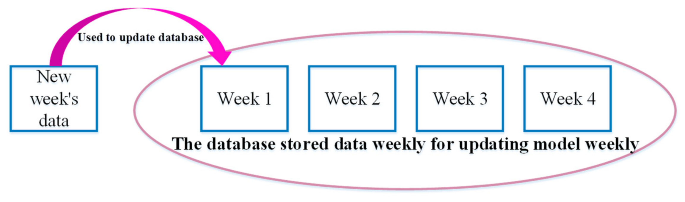
3.5. Update the Building Dynamics Model Regularly

Due to the thermophysical properties of the building and the operating condition of the equipment are not invariable, the accuracy of the control effect may decrease along with time going. Considering updating the system control model online in real-time will consume generous computing resources and augment the input costs, the offline prediction method is developed to update the model in this work. Too little data will lead to incomplete model coverage, while too much data will lead to long calculation time. Therefore, only appropriate amount of learning data can establish an accurate model through faster computation time. After accuracy verification by using different amounts of data, taking one month of data is considered to be a more reasonable method to identify the model. At the same time, the system operation state data are collected weekly to update the model database as shown in Figure 6. In other words, the data of the latest month is adopted to update the model every week and the precision of the controller can be improved effectively through continuous update of data variation.

4. Case Study

This section introduces a case study applying the adaptive MPC for the hybrid conditioning system heating.

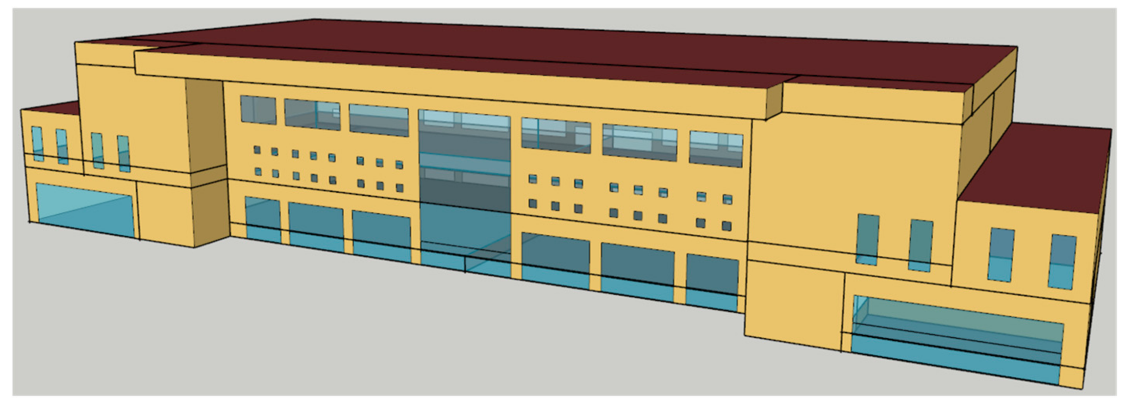
4.1. Target Building

The designed MPC controller will be applied to a high-speed railway station located in Zedang, China. Figure 7 shows the building model of Zedang Railway station built in SketchUp. The station has two floors and a total area of 14,970 m², including waiting halls, a ticket hall and a concourse, and the maximum number of passengers gathered is 1500 persons. An integrated model of the building was developed in TRNSYS, but only the first waiting hall on the first floor is presented later, the simulation and control methods for other zones are similar.

4.2. Geometrical and Envelope Description

The first waiting hall (L × W × H: 96 m × 26 m × 6 m), the research object of this paper, has only one north-facing exterior wall (96 m × 6 m) and the other three sides are interior walls. In addition, the window–wall ratio of the north-facing wall is 0.35. Envelope constitutions and U-values are described in

Table 1. Envelope constitution.

Envelope	Constitutions	Total U-Value (W/(m2·K))
External wall	Cement mortar 0.04 m	0.32
	Insulating material 0.08 m
	concrete hollow block 0.3 m
Internal wall	Cement mortar 0.04 m	0.71
	Insulating material 0.04 m
	Aerated concrete block 0.05 m
Overhead floorslab	Cement mortar 0.04 m	0.67
	Reinforced concrete 0.2 m
	Insulating material 0.04 m
Floor	Cement mortar 0.02 m	0.12
	Insulating material 0.04 m
	Reinforced concrete 0.12 m
	compacted clay 0.2 m
Windows	Double glazing of 0.006 m width for	2.4
	each glazing and 0.012 m air space
Glass curtain wall	Double low-E glazing of 0.006 m width for	1.9
	each glazing and 0.012 m air space

.

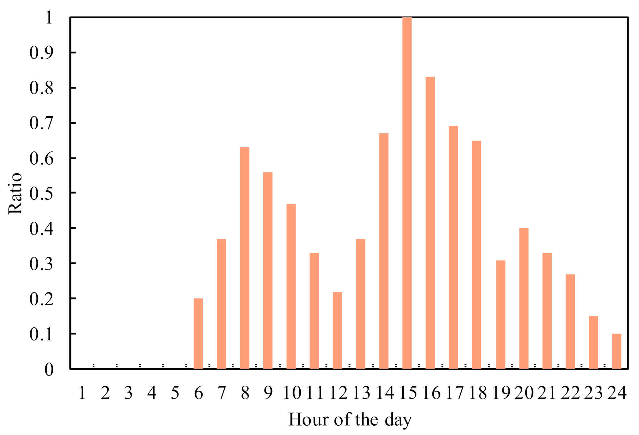
4.3. Internal Heat Gains

The internal heat gains of the zone include occupants, lighting system and appliances. According to the design scheme, the maximum number of passengers gathered in the first waiting hall is 1000 persons, i.e., 0.4 people per m². The sensible heat release of each person who is seated or has light work is supposed to be 115 W. The internal gains of lights are 15 W/m² and appliances are 20 W/m². Pursuant to the research group’s previous investigation on high-speed railway stations, the schedule for occupancy rate of the waiting hall is shown in Figure 8. The ratio denotes the current occupancy divided by the sizing value. As presented, the station is closed from 0 a.m. to 6 a.m., with maximum passenger flow at 2 p.m.

4.4. Air Infiltration

Due to the large space and the number of openings, the air infiltration of the railway station should not be ignored in the process of building simulation. The average air change rate of the waiting hall is set to 3.2 h⁻¹ in winter based on previous survey [33].

4.5. Heating System

As shown in Figure 9, the monthly mean temperature of the project site is low throughout the year. Even in summer, the highest average monthly temperature is only 15.8 °C. According to the calculation of indoor temperature throughout the year, the indoor average temperature in summer is lower than 27 °C. Therefore, only heating condition is considered instead of cooling condition in this area. Figure 10 shows the schematic diagram of the waiting hall heating system. The terminal of the hybrid air conditioning system consists of the radiant floor system and air diffusers. As for the design parameters of the radiant floor pipe network, pipe outside diameter, pipe spacing and filling layer thickness are 20 mm, 300 mm and 60 mm, respectively. The all-air system includes two air-handling units and 51 air diffusers with the designed total air supply volume is 21,600 m³/h. The temperature of the supply water to floor radiation system is set to 45 °C and all-air system is set to 60 °C considering that the radiant floor temperature should not be too high [34]. The heating is supplied by carbon dioxide air-source heat pumps (ASHP) which can provide two different temperatures of hot water by different heating methods and there are two pumps to power the water supply. The specific performance parameters of equipment are presented in Section 4.7.

4.6. Determination of Indoor Design Parameter

The predicted mean vote (PMV) model proposed by Fanger is one of the popular measures to evaluate thermal comfort conditions in buildings [35], which is related to the following six parameters: metabolic rate, clothing insulation, air temperature, mean radiant temperature, air velocity and air relative humidity [36]. According to ASHRAE Handbook [37], operative temperature T_op which is the indoor thermal comfort control variable is calculated by Equation (26).

$$T_{op} = \frac{h_{co}{T}_a+h_r{\overline{T}}_r}{h_{co}+h_r}$$

(26)

where T_a, ${\overline{T}}_r$, h_co and h_r are the ambient air temperature, mean radiation temperature, the coefficient of convective heat transfer and linear radiative heat transfer, respectively.

In order to establish the relationship of PMV and operative temperature, metabolic rate, clothing insulation, air velocity and air relative humidity can be considered as constant values. The metabolic rate is chosen as 115 W, as illustrated before. The clothing insulation of winter can be taken as 1.5, indoor air velocity as 0.15 m/s and air relative humidity as 40%. As shown in Figure 11, according to the actual building model developed in TRNSYS, PMV and operative temperature under the action of the hybrid air conditioning system present an obvious linear relationship.

The linear regression formula is shown as Equation (27) and the coefficient of determination (R²) is 0.9948.

$$\mathrm{PMV}=0.174T_{op}-3.4665$$

(27)

For general comfort, the range of value for PMV is taken as −0.5 to 0.5 [36]. Considering the energy saving of air-conditioning system, PMV value could be taken as negative deviation, that is, PMV is taken as −0.5 to 0 from Figure 11. The corresponding operative temperature T_op is calculated as 17 °C to 20 °C. In consequence, the indoor operative temperature is expected to remain between 17 °C and 20 °C when the air conditioning system is in operation in winter.

4.7. Determination of System Energy Consumption

The power consumptions of components are air-source heat pumps, water pumps of radiant terminal and all air-system and fans of air handling units. In addition, the specific energy consumption is calculated as follows.

4.7.1. Power Consumption of ASHP

The ASHP nominal COP is 3.31 (When the ambient temperature T_a and the supply water temperature is 5 °C, 60 °C, respectively) and the relationship between COP and ambient temperature can be obtained as Equation (28) from the manufacturer’s sample. When the supply water temperature is 45 °C for radiant floor heating system, the correction factor of 1.2 will be used for COP calculation as Equation (29). The power consumption of ASHP W_ASHP is calculated as Equation (30).

$${\mathrm{COP}}_{60°\mathrm{C}}=-5\times {10}^{-5}{T}_a^3-0.0024T_a^2+0.028T_a+3.2259$$

(28)

$${\mathrm{COP}}_{45°\mathrm{C}}=1.2{\mathrm{COP}}_{60°\mathrm{C}}$$

(29)

$$W_{\mathit{ASHP}}=\frac{Q_{\mathit{ASHP}}}{\mathrm{COP}}$$

(30)

where Q_ASHP refers to the supplied heating load by ASHP.

4.7.2. Power Consumption of Pump and Fan

Two frequency conversion pumps are applied to the water system. The design flowrate of a single pump is 55 m³/h, design head is 35 m and the rated power is 7.5 kW. According to the manufacturer’s measurement data, the curve equation of power change with volume flow rate is presented as Equation (31).

$$W_{\mathit{pump}}=-0.000005109363{\mathrm{m}}^3+0.00037254{\mathrm{m}}^2+0.0679\mathrm{m}+2.07$$

(31)

The fan of AHU operates at a fixed frequency, so the power W_fan is a constant value as 22 kW. Based on the above analysis, total system energy consumption is calculated as Equation (32), which is as the optimization objective in this paper.

$$W_{\mathit{total}}=W_{\mathit{ASHP}}+W_{\mathit{pump}}+W_{\mathit{fan}}$$

(32)

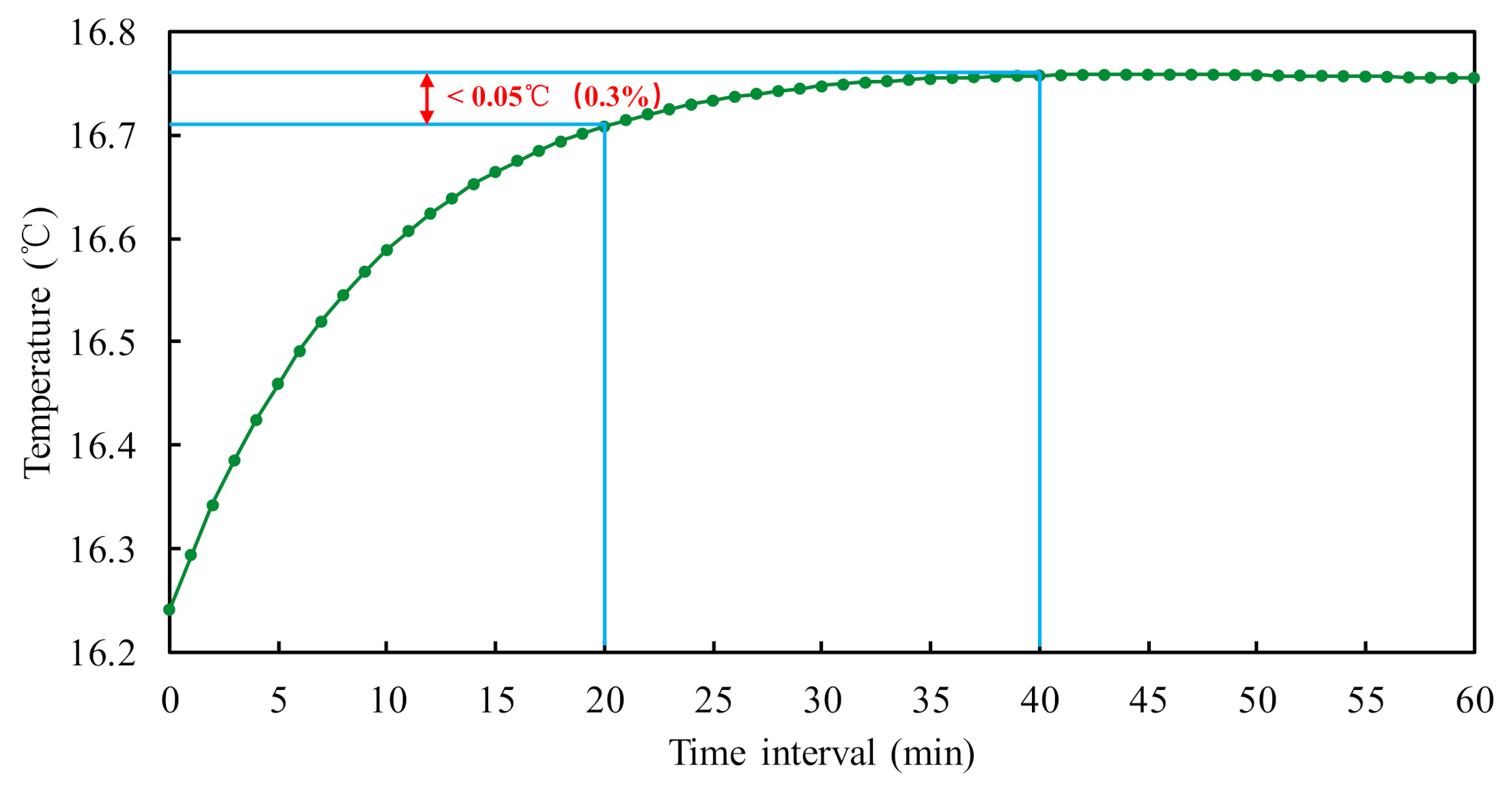
4.8. Determination of Sampling Time and Prediction Horizon

Due to the thermal inertia of the building, when the air conditioning system status changes, the indoor temperature cannot reach a steady-state immediately. Control errors will be caused if the air conditioning system changes before the indoor state reaches stability. Therefore, a simulation of building thermal inertia is realized in TRNSYS. As shown in Figure 12, a control signal is applied at time zero and the variation of zone operative temperature per minute is sampled. When 20 min later, the temperature gradually tends to be stable and the error from the final temperature is less than 0.05 °C (0.3%). As a result, the sampling and controlled time T_s are specified as 20 min. The result of the optimization is a series of control actions over the overall prediction horizon N and it is specified as 72, i.e., 24 h, which corresponds to an MPC horizon of one day.

4.9. Parameter Substitution

In order to achieve more accurate prediction and control, disturbance and control variables need to be replaced in the model. Assuming that the internal gains of lighting and equipment are constant, the change of total internal gains Q_inter is mainly related to the variation of passenger flow N_p. Due to the temperature of hot water supplied is a definite value, the amount of heating is related to the flow volume of water. Therefore, the disturbance vector can be converted to d = [T_o I_solar N_p]^T; the input vector can be converted to u = m_FL or u = [m_AS m_FL]^T. m_AS and m_FL are the flow volume of hot water to the air handling unit and radiant floor heating system, respectively.

4.10. Data Acquisition and Identification

The initial identification data is gathered from the TRNSYS model at 20-min intervals from 1 January to 31 January based on flow control under various weather conditions. By given the input and output data set, the contents of matrices A_d, B_d and E_d can be identified. One of the most convenient and accessible off-the-shelf solutions for the identification of mathematical models is the System Identification Toolbox [38]. The subspace model identification (SMI) method is supplied to identify the state space models. SMI is characterized by identifying the linear time-invariant state space model directly from the input and output data and obtaining the prediction model from the intermediate process. On the basis of u_k and y_k data set which is measured, the predicted output can be obtained by recursive iteration of the state space model [39]. Figure 13 shows results for the indoor operative temperature and the temperature of floor surface and inner surface of wall obtained using raw data and the parameter identification model for one month. Root mean square error (RMSE) is employed to estimate the prediction deviation. The RMSEs of indoor operative temperature, floor surface temperature and inner surface of wall temperature between raw simulative data and identification model data are 0.24 °C, 0.46 °C and 0.39 °C, respectively. It can be seen that the results of parameter identification model match the TRNSYS simulation perfectly.

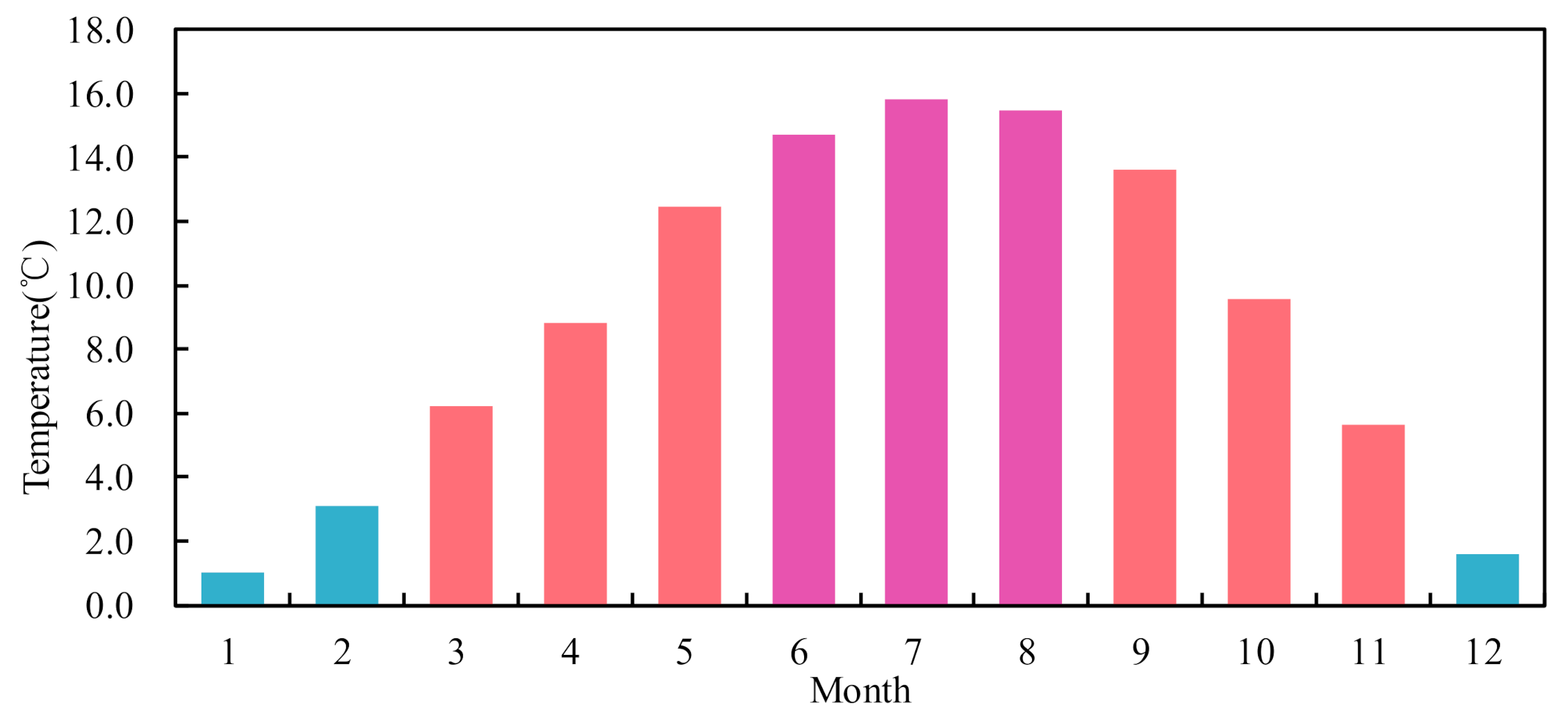
4.11. Prediction of Weather Data and Occupancy

Accurate prediction of disturbance variables is necessary for the zone thermal dynamic model and performance of the control system. Considering that the local meteorological data of the building site are affected by the surrounding environment, a meteorological observation station will be installed on the roof of the building to collect real-time weather data and modify the predicted weather data. The passenger flow in the waiting hall which is affected by the running time of the train can be predicted according to the historical data and modified with the real-time data.

5. Simulation Results and Discussion

A TRNSYS-MATLAB co-simulation testbed is developed to verify the system performance of the control strategy. The state parameters of the building calculated by TRNSYS at the sampling time are obtained by the MPC controller in MATLAB and then the controller output command signals to the heating system to regulate the indoor environment. Specific results and discussions are shown below.

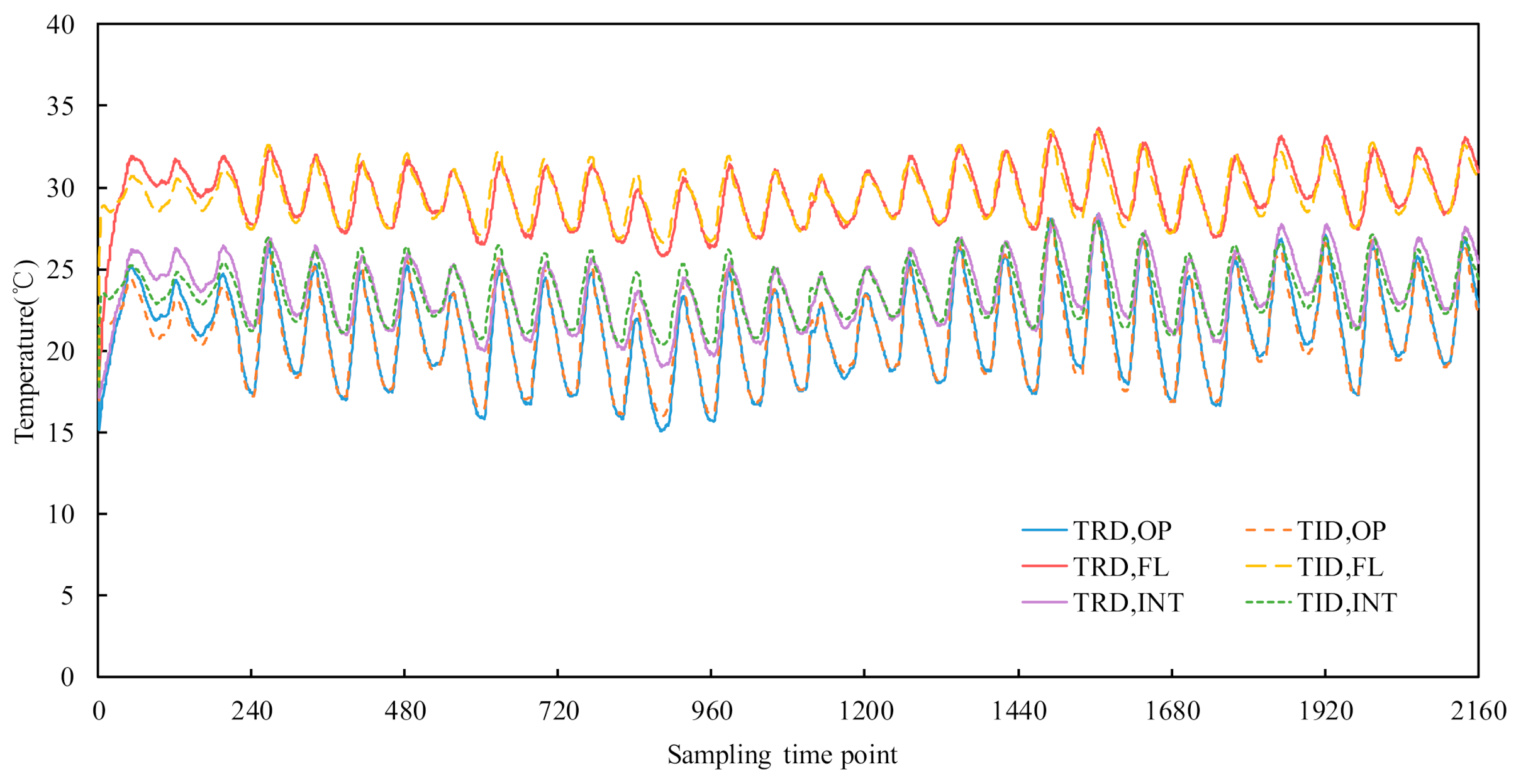
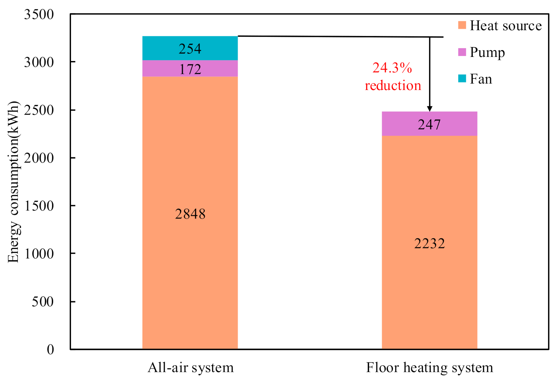
5.1. Comparison of Performance between Radiant Floor Heating and All-Air System

To verify that the radiant floor heating system is more energy efficient than the all-air system when there is only one system for heating and the reasonability of control principle that the radiant floor heating system is preferred and the insufficient heating quantity is provided by the all-air system as mentioned in Section 3, two kinds of systems are, respectively, applied for zone heating under partial load conditions based on MPC of one day. The indoor operative temperature and energy consumption comparisons are shown in Figure 14 and Figure 15, respectively. The simulation results show that both radiant floor heating and all-air system can maintain the operative temperature inside the comfort bound with few violations. For the all-air system, when the air-conditioning system is turned on, the indoor air temperature increases rapidly from 6:00 to 10:00. The maximum temperature variation occurs at about 14:00 and 17:00 with about 3 °C fluctuation. In addition, for the radiant floor heating system, the indoor air temperature varies gradually increase or decrease with lower temperature fluctuations and the radiant floor heating system achieves 24.3% reduction in energy consumption compared to the all-air system. The reason is that the concrete slab has higher thermal capacity compared to the air. In addition, the slowly changing floor temperature results in an equally slow change in indoor operative temperature. At the same time, all-air system leads to higher indoor temperature that causes more heat loss to the outside and the energy consumption of the fans is huge. Therefore, all=air system consumes more energy than the radiant floor heating system. This provides a reference basis for the preferential use of the radiant floor heating system.

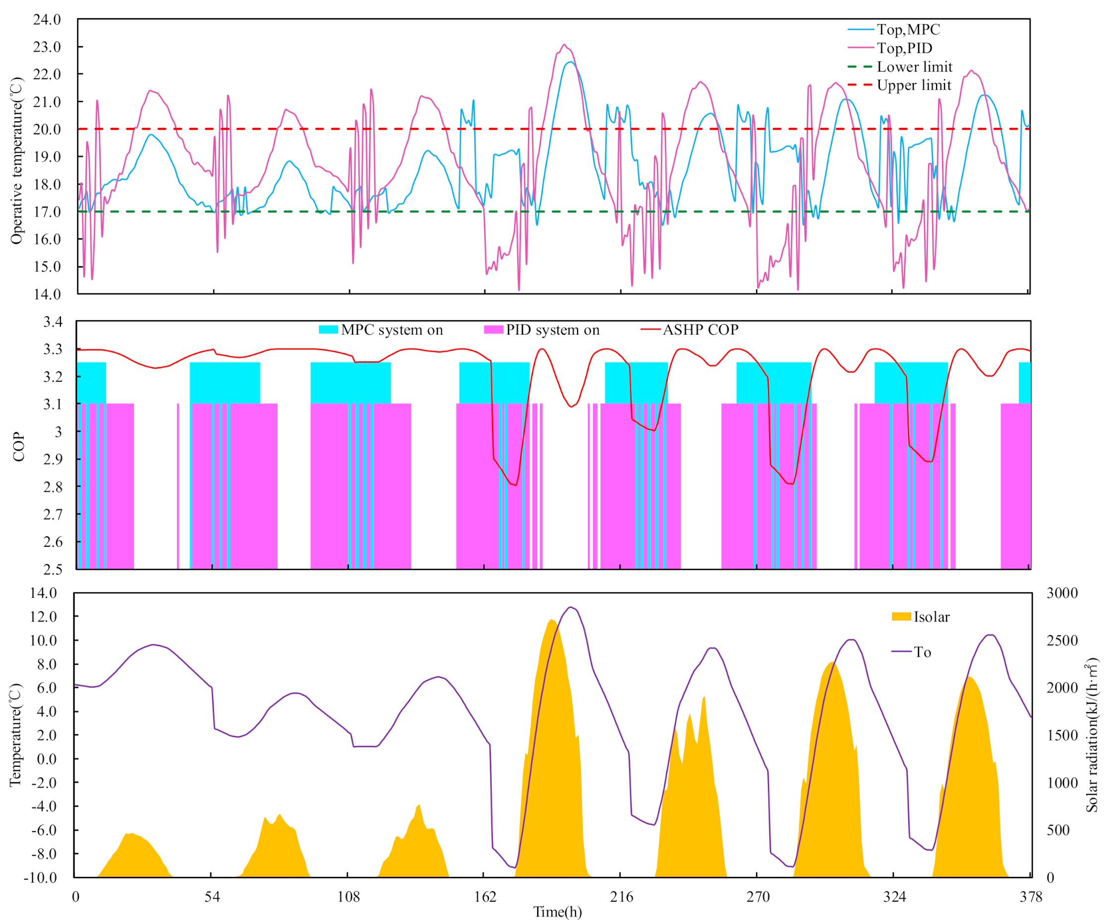
5.2. Comparison of Performance between the Adaptive MPC and PID Control

The performance of the adaptive MPC is evaluated by comparing with the PID control, the control system adjusts the water supply flow of the air-conditioning system according to the set the minimum operative temperature, i.e., 17 °C. What needs illustration is that the simulation covered the entire heating season, but only one week of data was shown for a clearer presentation of the variation in indoor operative temperature and other parameters. Figure 16 presents the operative temperature profiles as well as turn on time of air-conditioning system, the COP of ASHP and outdoor disturbance (ambient temperature and incident solar radiation). As shown, when the system adopts the adaptive MPC and the air conditioning is on, most time have acceptable thermal comfort temperature performance with fewer than 36 exceptions (9.5% violations) and a typical violation error is less than 0.5 °C, while using PID controller, there are 80 exceptions (21.2% violations) and a typical violation error is more than 2.5 °C. The ratio of the operating time of the air-conditioning system to the total service time of the station is 50.0% using the adaptive MPC and is 59.2% using the PID control. By exploiting the building model and disturbances prediction, MPC can preheat the zone before the temperature drop occurs. This makes the indoor temperature basically maintained within the thermal comfort range. At the same time, the relatively stable indoor temperature also reduces the opening time of the air conditioning system. An analysis is carried out to find out why the temperature exceeded range somewhat when the system was operating using MPC method: At the time of ambient temperature and passenger flow are low, a sizable amount of heat is required to maintain indoor thermal comfort. In the initial stage of the design, the system heating capacity will be allowed to be slightly inadequate in some extreme weather conditions due to the purpose of maximizing equipment utilization efficiency and saving cost. Therefore, insufficient heat supply results in the indoor operative temperature below the design value in some cases. On the other hand, due to the use of soft constraints, the temperature would be higher than the upper bound when the outdoor temperature is relatively high with high COP of ASHP to increase the heat storage of the zone and reduce total energy consumption during system start-up time. Meanwhile, some unknown random interference and the inaccuracy of prediction will also impinge the control accuracy [7]. As for PID control, the controller only acts as soon as a control error between original set point and actual zone operative temperature has occurred. Because of the thermal inertia of the building, the variation of the flow of people and weather conditions, the control cannot timely adjust the indoor temperature, resulting in further error.

The distribution of indoor operative temperature measured is also plotted as box-and-whisker diagrams in Figure 17. It shows that the mean operative temperature of MPC is 18.7 °C, for comparison, that is almost uniformly of PID with 18.8 °C. However, the interquartile range and the lower and upper bound of PID are broader than MPC, illustrating the MPC method can ensure a longer period of thermal comfort in the zone with lower temperature fluctuations.

Figure 18 shows the energy consumption performance of the heat source, pump and fan in two cases for the whole heating season. It presents that the total energy consumption reduces from 694,985 kWh of the PID control to 540,961 kWh of the adaptive MPC, achieving a 22.2% energy saving rate by the MPC as compared to the PID among which the heat source, pump and fan are reduced by 23.6%, 13.1% and 11.7%, respectively.

5.3. Comparison of Performance between the Adaptive MPC and Initial MPC

The initial MPC controller adopts the invariant state space equations obtained by original simulation data. To test the performance of initial MPC and adaptive MPC, a simulation was conducted in TRNSYS. Figure 19 shows the number of sampling time points outside the thermal comfort temperature range between the initial MPC and the adaptive MPC that updates state space equations weekly. Two models have the same violations on the first week as the two models are essentially the same on that week. However, from the second week onwards, the violations of the adaptive MPC present a general trend of reduction over time. This is because the adaptive MPC is being updated periodically by the off-line model adaption method as described in Section 3.5, leading to the prediction accuracy of the adaptive model is greatly improved. However, due to the limitation of the model, the reduction percentage of violations remains around a relatively fixed value after the ninth week and will not decrease anymore. Figure 20 shows the total energy consumption of the two cases, suggesting that the adaptive MPC achieves 11.5% reduction as compared to the initial MPC for the whole heating season due to the more accurate model predictions. The results of analysis and comparison are illustrated that the adaptive MPC has generally superior prediction performance and energy saving compared to the MPC without model update.

6. Conclusions

This paper presented an adaptive model predictive control for hybrid air conditioning heating to address the problems of indoor thermal comfort and energy consumption in the railway passenger station on Tibetan Plateau. A grey-box dynamic thermal model based on thermal-electrical analogy was developed, identified and updated to predict the thermal dynamics of the waiting hall in the station and the simulation of different controllers was implemented in a TRNSYS-MATLAB co-simulation testbed. Then, the control performance of the system was evaluated under different weather and occupancy conditions and compared against PID control and initial MPC method. The results can be summarized as follows:

• For the hybrid air conditioning system, the preferential use of radiant floor heating has greater energy saving potential than the preferential use of all-air system based on the MPC strategy.
• In terms of thermal comfort, the adaptive MPC achieves 90.5% indoor operative temperature satisfaction rate with lower temperature fluctuations benefited by the solution of time delay, whereas the PID control could only achieve 79.8%.
• In terms of energy-saving, the adaptive MPC achieves 22.2% energy consumption reduction as compared to the PID control for the system. It can be demonstrated that the MPC is superior to the PID control in temperature control and energy saving due to its advanced optimal control algorithm.
• The adaptive MPC achieves better indoor thermal comfort and 11.5% energy-saving as compared to the initial MPC with more accurate forecasting models which clarify the importance of updating the control model in time.

The MPC system proposed in this paper is based on a single zone in the railway station. For the design of control system with multiple zones, hydraulic balance, load distribution and collaborative optimization of multiple units should also be considered. In addition, it is necessary for us to further study the problem of appropriate correction and valve control according to the different positions of measuring points in practical engineering application.

References

1. Annual Development Report of China’s Building Energy Efficiency in 2020; Building Energy Conservation Research Center, Tsinghua University: Beijing, China, 2020.
2. Li, L.; Ma, W.; Chen, Z. Energy Consumption Factors Analysis and Energy Saving Measures Research of Modern Railway Passenger Station; China’s Railway Ministry Press: Beijing, China, 2010.
3. Shengwei, W.; Zhenjun, M. Supervisory and optimal control of building HVAC systems: A review. HVAC&R Res. 2008, 14, 3–32. [Google Scholar]
4. Afram, A.; Janabi-Sharifi, F. Theory and applications of HVAC control systems—A review of model predictive control (MPC). Build. Environ. 2014, 72, 343–355. [Google Scholar] [CrossRef]
5. Martin, K.; Michal, K. MPC-Based Reference Governors; Springer: Cham, Switzerland, 2019. [Google Scholar]
6. Zhang, D.; Huang, X.; Gao, D.; Cui, X.; Cai, N. Experimental study on control performance comparison between model predictive control and proportion-integral-derivative control for radiant ceiling cooling integrated with underfloor ventilation system. Appl. Therm. Eng. 2018, 143, 130–136. [Google Scholar] [CrossRef]
7. Hu, M.; Xiao, F.; Jorgensen, J.B.; Li, R. Price-responsive model predictive control of floor heating systems for demand response using building thermal mass. Appl. Therm. Eng. 2019, 153, 316–329. [Google Scholar] [CrossRef]
8. Joe, J.; Karava, P. A model predictive control strategy to optimize the performance of radiant floor heating and cooling systems in office buildings. Appl. Energy 2019, 245, 65–77. [Google Scholar] [CrossRef]
9. Yang, S.; Wan, M.P.; Ng, B.F.; Zhang, T.; Babu, S.; Zhang, Z.; Chen, W.; Dubey, S. A state-space thermal model incorporating humidity and thermal comfort for model predictive control in buildings. Energy Build. 2018, 170, 25–39. [Google Scholar] [CrossRef]
10. Afram, A.; Janabi-Sharifi, F. Supervisory model predictive controller (MPC) for residential HVAC systems: Implementation and experimentation on archetype sustainable house in Toronto. Energy Build. 2017, 154, 268–282. [Google Scholar] [CrossRef]
11. Sturzenegger, D.; Gyalistras, D.; Morari, M.; Smith, R.S. Model Predictive Climate Control of a Swiss Office Building: Implementation, Results, and Cost-Benefit Analysis. IEEE Trans. Control Syst. Technol. 2016, 24, 1–12. [Google Scholar] [CrossRef]
12. Aswani, A.; Master, N.; Taneja, J.; Culler, D.; Tomlin, C. Reducing Transient and Steady State Electricity Consumption in HVAC Using Learning-Based Model-Predictive Control. Proc. IEEE 2012, 100, 240–253. [Google Scholar] [CrossRef]
13. Huang, H.; Chen, L.; Hu, E. A new model predictive control scheme for energy and cost savings in commercial buildings: An airport terminal building case study. Build. Environ. 2015, 89, 203–216. [Google Scholar] [CrossRef]
14. O’Dwyer, E.; Cychowski, M.; Kouramas, K.; De Tomasi, L.; Lightbody, G. Scalable, Reconfigurable Model Predictive Control for Building Heating Systems. In Proceedings of the 2015 European Control Conference (ECC), Linz, Austria, 15–17 July 2015; pp. 2248–2253. [Google Scholar]
15. Ferreira, P.M.; Ruano, A.E.; Silva, S.; Conceicao, E.Z.E. Neural networks based predictive control for thermal comfort and energy savings in public buildings. Energy Build. 2012, 55, 238–251. [Google Scholar] [CrossRef] [Green Version]
16. Li, X.; Zhao, T.; Zhang, J.; Chen, T. Predication control for indoor temperature time-delay using Elman neural network in variable air volume system. Energy Build. 2017, 154, 545–552. [Google Scholar] [CrossRef]
17. Zeng, Y.; Zhang, Z.; Kusiak, A. Predictive modeling and optimization of a multi-zone HVAC system with data mining and firefly algorithms. Energy 2015, 86, 393–402. [Google Scholar] [CrossRef]
18. Afram, A.; Janabi-Sharifi, F. Gray-box modeling and validation of residential HVAC system for control system design. Appl. Energy 2015, 137, 134–150. [Google Scholar] [CrossRef]
19. Derakhtenjani, A.S.; Candanedo, J.A.; Chen, Y.; Dehkordi, V.R.; Athienitis, A.K. Modeling approaches for the characterization of building thermal dynamics and model-based control: A case study. Sci. Technol. Built. Environ. 2015, 21, 824–836. [Google Scholar] [CrossRef]
20. Wang, D.; Liu, Y.; Wang, Y.; Liu, J. Numerical and experimental analysis of floor heat storage and release during an intermittent in-slab floor heating process. Appl. Therm. Eng. 2014, 62, 398–406. [Google Scholar] [CrossRef]
21. Wang, Z.; Luo, M.; Geng, Y.; Lin, B.; Zhu, Y. A model to compare convective and radiant heating systems for intermittent space heating. Appl. Energy 2018, 215, 211–226. [Google Scholar] [CrossRef]
22. Afram, A.; Fung, A.S.; Janabi-Sharifi, F.; Raahemifar, K. Development of an accurate gray-box model of ubiquitous residential HVAC system for precise performance prediction during summer and winter seasons. Energy Build. 2018, 171, 168–182. [Google Scholar] [CrossRef]
23. O'Dwyer, E.; De Tommasi, L.; Kouramas, K.; Cychowski, M.; Lightbody, G. Modelling and disturbance estimation for model predictive control in building heating systems. Energy Build. 2016, 130, 532–545. [Google Scholar] [CrossRef]
24. Zajic, I.; Larkowski, T.; Sumislawska, M.; Burnham, K.J.; Hill, D. Modelling of an Air Handling Unit: A Hammerstein-bilinear Model Identification Approach. In Proceedings of the 21st International Conference on Systems Engineering, Las Vegas, NV, USA, 16–18 August 2011; pp. 59–63. [Google Scholar]
25. Yang, S.; Wan, M.P.; Chen, W.; Ng, B.F.; Zhai, D. An adaptive robust model predictive control for indoor climate optimization and uncertainties handling in buildings. Build. Environ. 2019, 163, 106326. [Google Scholar] [CrossRef]
26. Yang, S.; Wan, M.P.; Chen, W.; Ng, B.F.; Dubey, S. Model predictive control with adaptive machine-learning-based model for building energy efficiency and comfort optimization. Appl. Energy 2020, 271, 115147. [Google Scholar] [CrossRef]
27. Mayne, D.Q. Model predictive control: Recent developments and future promise. Automatica 2014, 50, 2967–2986. [Google Scholar] [CrossRef]
28. Woolley, J.; Schiavon, S.; Bauman, F.; Raftery, P.; Pantelic, J. Side-by-side laboratory comparison of space heat extraction rates and thermal energy use for radiant and all-air systems. Energy Build. 2018, 176, 139–150. [Google Scholar] [CrossRef] [Green Version]
29. Karmann, C.; Schiavon, S.; Bauman, F. Thermal comfort in buildings using radiant vs. all-air systems: A critical literature review. Energy Build. 2017, 111, 123–131. [Google Scholar] [CrossRef] [Green Version]
30. Liu, H.; Hu, F.; Su, J.; Wei, X.; Qin, R. Comparisons on Kalman-Filter-Based Dynamic State Estimation Algorithms of Power Systems. IEEE Access 2020, 8, 51035–51043. [Google Scholar] [CrossRef]
31. Xu, W. Technical Specification for Floor Radiant Heating and Cooling; China Architecture & Building Press: Beijing, China, 2012. [Google Scholar]
32. Lofberg, J. YALMIP: A Toolbox for Modeling and Optimization in MATLAB. In Proceedings of the IEEE International Conference on Robotics and Automation, Taipei, Taiwan, 2–4 September 2004. [Google Scholar]
33. Qian, B.; Yu, T.; Bi, H.; Lei, B. Measurements of Energy Consumption and Environment Quality of High-Speed Railway Stations in China. Energies 2020, 13, 1681. [Google Scholar] [CrossRef] [Green Version]
34. Khorasanizadeh, H.; Sheikhzadeh, G.A.; Azemati, A.A.; Hadavand, B.S. Numerical study of air flow and heat transfer in a two-dimensional enclosure with floor heating. Energy Build. 2014, 78, 98–104. [Google Scholar] [CrossRef]
35. Fanger, P.O. Thermal Comfort: Analysis and Applications in Environmental Engineering; McGraw-Hil: New York, NY, USA, 1972. [Google Scholar]
36. ASHRAE. Thermal Environmental Conditions for Human Occupancy; ANSI/ASHRAE Standard 55-2017 2017; ASHRAE: Atlanta, GA, USA, 2017. [Google Scholar]
37. ASHRAE. ASHRAE Handbook of Fundamentals; ASHRAE: Atlanta, GA, USA, 2017. [Google Scholar]
38. The Mathwork. System Identification Toolbox. Available online: https://www.mathworks.com/help/ident/index.html?s_tid=srchtitle (accessed on 3 January 2021).
39. Verhaegen, M.; Deprettere, E. A Fast, Recursive MIMO State Space Model Identification Algorithm. In Proceedings of the 30th IEEE Conference on Decision and Control, Brighton, UK, 11–13 December 1991; pp. 1349–1354. [Google Scholar]
Figure 1. An overview of the methodology for developing the MPC system.
Energies 14 01996 g001
Figure 2. Framework of MPC system.
Energies 14 01996 g002
Figure 3. Internal logic of MPC controller.
Energies 14 01996 g003
Figure 4. Energy balance diagram of heat exchanger.
Energies 14 01996 g004
Figure 5. RC model of the integrated system.
Energies 14 01996 g005
Figure 6. Database update process.
Energies 14 01996 g006
Figure 7. Building model of Zedang Railway station.
Energies 14 01996 g007
Figure 8. Schedules for occupancy.
Energies 14 01996 g008
Figure 9. Monthly mean temperature of Zedang.
Energies 14 01996 g009
Figure 10. Schematic diagram of the heating system.
Energies 14 01996 g010
Figure 11. Relationship between PMV and operative temperature.
Energies 14 01996 g011
Figure 12. Variation curve of operative temperature with time.
Energies 14 01996 g012
Figure 13. Indoor operative temperature, floor surface temperature and inner surface of wall temperature obtained using raw data and the parameter identification model.
Energies 14 01996 g013
Figure 14. Indoor operative temperature comparison between radiant floor heating and all-air system.
Energies 14 01996 g014
Figure 15. Energy consumption comparison between radiant floor heating and all-air system.
Energies 14 01996 g015
Figure 16. Performance comparison between the adaptive MPC and PID control.
Energies 14 01996 g016
Figure 17. Statistical distributions of indoor operative temperature comparison.
Energies 14 01996 g017
Figure 18. Energy consumption performance comparison.
Energies 14 01996 g018
Figure 19. Violations of thermal comfort temperature range by the initial and adaptive MPC.
Energies 14 01996 g019
Figure 20. Total energy consumption comparison of the two cases.
Energies 14 01996 g020