A New Lumped Approach for the Simulation of the Magnetron Injection Gun for MegaWatt-Class EU Gyrotrons

Abstract

In the framework of the ITER (International Thermonuclear Experimental Reactor) project, one of the key components of the reactor is the ECRH (Electron Cyclotron Resonance Heating). This system has the duty to heat the plasma inside the tokamak, using high frequency and power radio waves, produced by sets of 1MW gyrotrons. One of the main issues related to the gyrotron operation is the output power drop that happens right after the beginning of a pulse. In this work, we study the underlying phenomena that cause the power drop, focusing on the gyrotron’s MIG (Magnetron Injection Gun) of the 1MW, 170 GHz European Gyrotron prototype for ITER. It is shown how the current emission and the temperature of the emitter are tightly bound, and how their interaction causes the power drop, observed experimentally. Furthermore, a simple yet effective lumped-parameter model to describe the MIG’s cathode thermal dynamics is developed, which is able to predict the power output of the gyrotron by simulating the propagation of the heat inside this component. The model is validated against test results, showing a good capability to reproduce the measured behavior of the system, while still being open to further improvements.

1. Introduction

In the framework of nuclear fusion research, a worldwide aggressive research program is addressing the main issues concerning the operation of magnetic-confinement devices, i.e., tokamaks [1], such as ITER (International Thermonuclear Experimental Reactor) [2], under construction in France or JT-60SA [3], under commissioning in Japan, and stellarators [4], such the Weldenstein 7X [5], under operation in Germany. For both kinds of configurations, for present and future machines, the plasma inside the vacuum chamber needs to be heated up to temperatures of 100–200 MK, which requires dedicated heating technologies. The Electron Cyclotron Resonance Heating (ECRH) is one of the plasma heating systems, and it consists of a cluster of MegaWatt-class gyrotron units [6], delivering power in the form of radiofrequency within the mm-range wavelength in continuous wave (CW) operation. The gyrotron tube used to heat plasma in the Weldenstein 7X reactor is shown in Figure 1 as an example.

Gyrotrons [6] are electron cyclotron masers, where electromagnetic energy (at a frequency near the electron cyclotron frequency or one of its harmonics) is radiated by a beam of weakly relativistic electrons, rotating (“gyrating”) in an external longitudinal magnetic field with a perpendicular velocity in the so-called resonator, which, in Figure 2a, is addressed as the “cavity”.

The gyrotron subsystem in charge of generating the beam current to produce the radio frequency (RF) wave is the Magnetron Injection Gun (MIG). This is composed of a central cathode and an external anode, mounted one inside the other, as shown in Figure 2a. Electrons emitted by the anode are accelerated inside the electric field produced by the application of a cathode–anode electric potential. They are then shaped into a hollow beam and guided towards the resonating cavity, by the powerful magnetic field generated by the superconducting magnet. Once the electron beam enters the cavity, the beam–wave interaction causes the generation of an RF-wave, which is then extracted and guided outside the device, by a series of mirrors, to be used in plasma-heating and other applications.

Focusing on the cathode, which is shown in detail in Figure 3, we can notice that it assumes a mushroom-like external shape, necessary for the correct shaping (together with the anode configuration) of the external electric field. The internal configuration is quite complex, with the presence of numerous thermal shields. This is due to the fact that the electron emission region must be extremely well-defined, to obtain the desired beam shape and device performance. Thus, only the emitter ring must be heated up, in order to emit electrons, while the surrounding components must be kept as cool as possible, to avoid spurious emissions from other regions of the cathode.

The emitter ring itself is made of a material which can withstand the high operational temperatures required and that promotes electron emission by having low material-to-vacuum work function. In the case of the European gyrotron for ITER [7,8], of special interest here, the emitter is constituted by a substrate of sintered tungsten impregnated by barium-calcium aluminate. To generate the amount of current necessary to drive, e.g., the 1MW ITER gyrotron, the surface of the emitter ring must reach temperatures of about 1200 K. An electrical heating element is placed purposely in the cavity formed by the emitter ring and the thermal shields, as shown in Figure 3, labeled as “Filament cavity”.

While the technology of gyrotrons is progressing in Europe [9] and around the world [6,10], some issues are still to be addressed and solved, to guarantee an optimized long-pulse operation at the full-rated power. Among them, as far as the MIG’s cathode is concerned, we find the design of a suitable control system to guarantee a constant current [11], which, in fact, tends to decay during the gyrotron operation, jeopardizing the device performance. During the long pulse tests performed on the 1MW, 170 GHz European Gyrotron prototype for ITER, for instance, it has been observed that the cathode current undergoes a drop of more than 20% over the course of few seconds, after the beginning of the shot [7,8,12]. Up to now, the main technique utilized to counteract this phenomenon consists in the pre-programming of heating sequences of the MIG’s cathode, to reach the desired current level during the gyrotron operation [11]. This technique has been proven effective for stabilizing the current during the testing of the device, since, by rising the heating power before the start of a pulse, it is possible to overcome the time delay associated with the heat propagation inside the system. This allowed the operators to maintain the emitter surface temperature and, thus, the emitted current, as steady as possible. However, when operating inside fusion plants, gyrotrons are required to be turned on and off without previous notice. This happens because their operation is subordinated to the control of the central system of the plant. Thus, pre-programming of the heating sequences is not suitable as a power-stabilization technique, since the instance in which gyrotrons must be turned on or off is not known in advance.

Different works over the control systems of vacuum tube devices have been carried on in the past over systems whose requirements differ substantially from the ones analyzed in this work, or for the stabilization of different parameters of high power gyrotrons. The work from Idehara et al. [13] describes the stabilization of the output power of gyrotrons used for high-power spectroscopy that, however, have a much faster response than MW lever fusion gyrotrons. Another relevant paper refers to the control of medium-sized RF sources for NMR spectroscopy devices, which, however, are continuously operated and thus require only long-term feedback stabilization of the operational parameters [14]. A lot of research [15,16] has been done, instead, on the frequency, mode, and phase stabilization of various sizes of gyrotron devices, but none focuses on the control of the thermal behavior of the MIG’s cathode.

In this work, we concentrate on the test-case of the MIG of a European gyrotron designed for ITER (1 MW and 170 GHz [7,8,12]), and we develop a lumped-parameter dynamic model for its cathode that is capable of capturing the physical phenomena that are responsible for the current drop in the gyrotrons, when operated at high power levels. The purpose behind the lumped model development is twofold: First, having a numerical model able to predict the evolution of the system can allow operators to calculate and implement in the experiments different sequences of input heating power, as to minimize the occurrence of the current drop when performing controlled tests. This would allow, for example, the performing of long shots with minimal presence of current drop and thus allow a full test with RF production on the gyrotron. The second purpose of this model is to have a simple tool that will allow us to verify the effects of the implementation of a suitable control system that is able to suppress undesired current decay.

The paper is organized as follows: First, we focus on the detailed description of the physics of thermionic emission in the operational regime of the gyrotron MIG, which is fully relevant for the current drop phenomenon. After the reason of the current decay is identified, the lumped-parameter thermal–electric model is presented and then validated by comparison with experimental data from the Fusion for Energy (F4E)’s FALCON facility, at the EPFL (École Polytechnique Fédérale de Lausanne) premises in Lausanne.

2. The MIG of the 1MW European Gyrotron for ITER

2.1. Geometry and Materials

In this section, with reference to Figure 3, we provide a detailed explanation of the geometry of the MIG’s cathode and the materials of which it is composed.

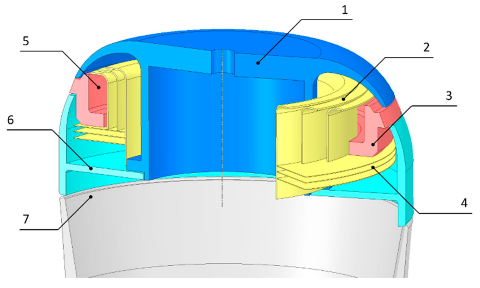
• The main component responsible for the electron emission is the emitter ring, which, in Figure 3, is labeled as element #3. The beam current generation occurs on its external surface, due to the thermionic effect. Here, due to their thermal agitation, electrons are able to overcome the material-vacuum potential barrier and leave the surface. To promote this phenomenon, the material of which the emitter ring is composed must be characterized by a low metal-vacuum work function. For this reason, this component is built using a sintered tungsten substrate which is impregnated with barium-calcium aluminate.
• To direct all the heat injected into the system towards the emitter ring, a set of thermal shields are mounted around the heating element, contained in the cavity formed by the emitter ring and the shields, labeled as #5 in Figure 3. The thermal shields themselves, labeled as #2 and #4, respectively, are made of polished and highly reflective material. This is due to the fact that the main mechanism of heat transfer between components is radiative heat transfer, since the cavity of the gyrotron is evacuated.
• Parts #1 (the nose cone) and #6 (the prolongator) in Figure 3 are used as a support for the emitter ring and for the thermal shields. Their shape and alignment are crucial for obtaining high efficiency in the RF power production, since they modify the electric field configuration inside the MIG. The electric field, together with the magnetic field, determine the direction of the electrons towards the resonant cavity and the shaping of the beam.

2.2. Working Conditions

Magnetron Injection Guns installed on vacuum tube devices to generate the beam current can be operated in two different regimes that depend on their working parameters [17,18]. The most common regime, in which small telecommunication tubes and the majority of scientific research apparatus work, is the Space Charge Limited (SCL) regime. Here the accelerating electric field inside the tube is not strong enough to drive away from the surface of the emitter all the electrons expelled due to the thermionic effect. This causes the formation of a charge cloud around the emitter ring, that limits the current below the value of the one emitted by pure thermionic effect. In this regime, raising or lowering the electric field influences directly the amount of electrons that manage to escape from the surface, and thus the beam current is dependent on the accelerating voltage applied between the electrodes [17]. This situation is represented by the black curve of Figure 4, named Lang–Blodgett.

The second regime is called Temperature Limited (TL) regime and is encountered in devices in which the accelerating potential is sufficiently high to drive away from the surface of the emitter all the electrons generated via the thermionic effect. When this regime is reached, a saturation effect is encountered, and raising the electric field does not affect the amount of electrons emitted by the cathode anymore. Only the temperature of the emitter is now affecting the number of electrons emitted per unit time, which is equal to the one emitted by thermionic effect [18]. This situation is shown by one of the colored curves of Figure 4, which shows the current saturation in the TL regime. The slight dependence of the current on the accelerating potential still present in the saturation zone is due to small variations in the work function of the metal when an electric field is applied to its surface. This phenomenon is studied in the next paragraphs.

The cathode working region depends fundamentally on three different parameters: the work function of the material that composes the emitting region, its surface temperature, and the value of the anode–cathode potential [17,18,19]. In Figure 3, we can observe a plot of the different regime as a function of the accelerating voltage. Below the black curve named “Lang–Blodgett”, the regime is TL, while the curve itself describes the SC regime. The colored curves represent different values of the emitted current in the TL regime for varying temperature of operation of the emitter ring, while the red square represents the expected region in which the MIG’s cathode operational parameters fall.

From this analysis, we can see that the operational regime of the electron gun can be identified as the temperature limited regime, and thus the emitted current will be fundamentally dependent on the temperature of the emitter region surface. The phenomenon can be described by the Richardson–Dushman equation [20] (Equation (1)).

$$J_{RD}=120T^{2}exp\left(-\frac{W_0+c·T- \mathsf{\Delta }W}{K_{b}T}\right) \left[\frac{A}{{\mathrm{cm}}^2}\right]$$

(1)

where $W_0$ represents the material work function, the term $c·T$ is a correction term that keeps into account the variation of the work function with temperature, and the term $\mathsf{\Delta }W$ implements into the model the Schottky lowering of the surface potential barrier due to the presence of an external electric field. All the terms are known from the material characteristics, except for the Schottky barrier lowering [19]. That term can be considered fixed and constant, since it is directly related to the value of the electric field on the surface of the emitter by Equation (2) [20]:

$$\mathsf{\Delta }W=-\sqrt{e^3\frac{E}{4\mathsf{\pi }{ϵ}_0}}\left[\mathrm{eV}\right]$$

(2)

which is itself directly related to the value of the anode–cathode applied voltage.

To retrieve the electric field value over the emitter surface, a finite-element simulation of the entire MIG was performed, using the software ANSYS^®. In Figure 5, an azimuthal slice of the full computational domain is shown, to allow for the visualization of the various boundaries. The actual simulation domain is composed of the whole portion of vacuum included between the MIG’s cathode and anode. The choice of simulating the whole domain instead of simplifying it comes from the fact that the equations solved in this case are simple, and a steady state simulation was performed. Thus, the computational effort in this case is low.

On this domain, the Poisson equation is solved, to retrieve the electric field value present on the cathode surface when operating at nominal conditions. The boundary conditions for our case are the following:

• A potential of −50 kV is applied to the MIG’s cathode, which, in Figure 5, is la-beled as #3.
• A potential of +30 kV is applied to the MIG’s anode, which is labeled as #2.
• On the flat top and bottom surfaces, labeled as #1 and #4, no boundary conditions are specified.

The results are reported in Figure 6, where the solution is sampled over the cells that compose the emitter ring surface, along the path shown in red in Figure 5. Here the electric field assumes a constant value of 4.9 kV/mm over most of the surface of the emitter ring and drops to lower values near its edges. With those electric field values, the Schottky lowering is in the order of 0.1 eV, which is enough to influence significantly the emitted current, due to the exponential nature of the equation [20].

From the Richardson–Dushman equation, the amount of heat that the electron current extracts from the emitting surface, when leaving it, can be computed. To do this, the current density is multiplied from the average electron energy [21], and thus the relation shown in Equation (3) is obtained:

$$q_p^{″}\left(T_c\right)=\left(W_0+2K_{b}T\right)·120T^{2}exp\left(-\frac{W_0+c·T-\mathsf{\Delta }W}{K_{b}T}\right)\left[\frac{W}{{\mathrm{cm}}^2}\right]$$

(3)

where $q_p^{″}$ is the cooling power per unit area associated to the electron emission phenomenon.

Following this simple analysis, we can deduce that the underlying cause to the current drop phenomenon observed during the gyrotron long pulse operation is in fact related to proportionality of the electron beam generated from the emitter surface on its temperature. When electrons are emitted, they remove some energy from the emitter, causing a lowering of the surface temperature and, thus, a drop in the current via a feedback phenomenon. After a certain amount of time, the system reaches an equilibrium, in which the cooling power of the beam is counterbalanced by the heat diffusing to the surface trough the material of which the emitter is composed.

3. A Lumped Model for the MIG’s Cathode Thermal Behavior and Current Emission

3.1. Justification for a Lumped-Parameter Model

To investigate if the choice of a lumped parameter model is suitable for the description of the European 170 GHz, 1MW gyrotron’s cathode, preliminary FEM (Finite Element Method) simulations were performed to inspect the temperature field inside the emitter ring and the other components. In particular, the software OpenFOAM [22] was utilized for simulating, in detail, the heat transfer between various parts of the system by implementing both conduction and radiation. For the second heat transfer mode, the Radiation Transfer Equation (RTE) was solved by using the implemented fvDOM model, which is based on the discrete ordinate method for solving directional-dependent transport equations [23,24].

The computational domain for the FEM simulation is shown in Figure 7 and is implemented with the classical wedge shape, which is the standard OpenFOAM model to represent axial-symmetric geometries [24]. This configuration was chosen over the complete revolved geometry for computation reasons, to reduce the CPU-time required for performing a single simulation. The domain is composed of several interacting bodies. They are surrounded by a vacuum, which is implemented in this simulation as low-pressure stationary air, with a fictitiously extremely low thermal conductivity (${10}^{-10}\left[\frac{W}{m·K}\right]$). Note that the stationarity for the air is imposed, to avoid errors caused by its buoyancy.

In each solid zone, thermal conduction is allowed. The heat-diffusion equation for isotropic materials is solved, subject to the thermal flux on the surfaces caused by the presence of radiation in the vacuum. In the fictitious fluid mimicking the vacuum, the heat conduction is modeled but negligible, and the radiation transport equation is solved, so that the ray intensity for each cell and every direction is retrieved. This is then combined to the surface radiative properties of the solids, to generate a boundary heat flux term in each of them.

Continuity of temperature field is imposed between any solids and the medium implementing the vacuum around them, and between touching solids. The latter condition is equivalent to ignore any thermal resistances in the contact area.

The initial conditions are imposed for the temperature and ray intensity field, and the whole MIG is assumed to be in thermal equilibrium, at room temperature.

The mesh quality is checked by using the OpenFOAM utility checkMesh [25], to verify that mesh metrics respect strict quality conditions for the solver to produce reliable results. The equations were solved by using a time-varying scheme, and the whole system was simulated for 2000s, time necessary for all the solid to reach a stable temperature.

To check to what extent the temperature of the emitter remains uniform, the time evolution of the temperature field under a step-wise input power of various amplitudes is analyzed first. As we can see, in Figure 8, for an input power of 300 W, the maximum difference in temperature amounts to just −0.39%, and it is found to be between the average and the minimum temperature of the body, showing that, over the course of the whole heating sequence of the emitter, from room temperature to the nominal one, the internal temperature field remains quite uniform. Figure 9 reports the maximum deviations from the average temperature for different values of the heating power, showing that even for the high-power levels, close to the maximum operative power allowed for the cathode heater, the deviation remains lower than 1%, which we judge acceptable for the implementation for a lumped parameter model.

A second analysis to assess the suitability of the lumped approximation to the modeling of the emitter was carried out, focusing on the effect of the beam on the temperature distribution in the emitter. As already discussed above, when an accelerating voltage is applied to the emitter ring, the consequent emission of electrons causes a rapid cooling of its surface. This temperature variation then propagates inside the material, causing the appearance of a radial temperature distribution.

To evaluate the error caused by approximating this temperature distribution with the lumped parameter model, the heat equation is solved in a simplified model on a cylindrical computational domain approximating the emitter configuration, as shown in Figure 10. Thanks to the symmetry of the system, the z and θ components in the equation were discarded, leaving only the radial component to be evaluated.

The integration domain is a simplification and schematization of the emitter thickness that will provide information on how the temperature wave propagates inside this component when the beam is turned on. On this domain, the material thermal conductivity is independent on time, position, and temperature.

The resulting problem for the simplified model is reported in Equation (4):

$$\left\{\begin{array}{cc}\rho c_p\frac{\partial T}{\partial t}=-k\frac{1}{r}\frac{\partial }{\partial r}\left(r\frac{dT}{dr}\right)\hfill & \mathit{for}r\in \left[r_I,r_I+\mathsf{\Delta }r\right],t\in \left(0,t_f\right]\hfill \\ T=T_0\hfill & \mathit{for}r\in \left[r_I,r_I+\mathsf{\Delta }r\right],t=0\hfill \\ \frac{\partial T}{\partial r}=0\hfill & \mathit{for}r=r_I,t\in \left(0,t_f\right]\hfill \\ -k\frac{\partial T}{\partial r}=q^{″}\left(T\left(r\right)\right)\hfill & \mathit{for}r=r_I+\mathsf{\Delta }r,t\in \left(0,t_f\right]\hfill \end{array}\right.$$

(4)

where $r_I$ is the radius of the internal surface of the emitter exposed to the filament, $\mathsf{\Delta }r$ is the thickness of the emitter ring measured from the internal surface to the emitting surface, and $q^{″}$ represents the heat flux removed from this last one by the electron beam, and its magnitude is computed according to Equation (3).

Equation (4) was solved numerically by discretizing the spatial 1st and 2nd order derivatives according to central finite difference schemes. The time derivative was discretized using the Backwards Euler scheme to improve stability at the cost of added computational time.

In Figure 11 the numerical solution to the problem is shown from t = 0 s to t = 10 s with timesteps of 1s. As expected, the low temperature wave propagates inward, cooling down all the material.

For each timestep, the average temperature inside the emitter is computed, and then the percent deviation of the maximum and minimum temperatures are calculated. The results are shown in Figure 12. Figure 12a shows the results for the whole simulation time, while Figure 12b is a zoom to highlight the detail of the variation happening in the initial times. It can be noted that, even in the first instants of the evolution, the temperature distribution that results from the beam-cooling effect in the solid is quite uniform, with a maximum deviation from the average temperature of −0.167%. This can be ascribed to the fact that the emitter presents a small size and a high thermal conductivity.

In view of the large temperature uniformity across the emitter, the analysis performed confirms the suitability of a lumped parameter approach, which subdivides the computational domain into a small number of regions described by a single temperature value, to model the thermal phenomena occurring inside the emitter ring with good precision. This happens because the temperature distributions in this object, generated both by the filament irradiation and by the beam cooling, are still quite uniform, thanks to the high thermal conductivity of the material and its reduced dimensions.

3.2. Implementation of the Lumped Model

Since the temperature of the exposed surface is the most important parameter that rules the intensity of the electron beam, the lumped model developed in the present paper focuses on the emitter ring, subdividing it in a limited number of sub-zones. In Figure 13a, a vertical section of the emitter component is shown, subdivided into six sub-zones, following its natural geometry. Each sub-zone in the lumped model is considered to have a uniform temperature, which might be different from that of the adjacent sub-zones. The zones can transfer heat with the surroundings by conduction and radiation, undergoing the following three phenomena:

• Thermal diffusion through the emitter, modeled for two generic adjacent zones i and j, using geometrical thermal resistances, according to Equation (4):

  $$R_{ij}=\frac{d}{k{A}_c}ln\left(\frac{r_2}{r_1}\right)\left[\frac{K}{W}\right]$$

  (5)

  if the two masses are adjacent along the radial direction, and:

  $$R_{ij}=\frac{d}{k{A}_c}\left[\frac{K}{W}\right]$$

  (6)

  if they are adjacent in the vertical direction. Here, $A_c$ is the contact area between two adjacent regions, and $d$ is the distance between their barycenter.
• Radiative heat transfer to the surroundings, modeled for the generic mass i according to the following equation:

  $$q_i^{″}=-K\mathsf{\sigma }{A}_i\left(T_i^4-T_{surr}^4\right)\left[\frac{W}{{\mathrm{m}}^2}\right]$$

  (7)

  where $A_i$ is the area of the exposed area of zone i, $\mathsf{\sigma }$ is the Stefan–Boltzmann constant and K is a constant parameter calculated numerically, to keep into account the geometry of the surroundings.
• Electron emission and subsequent cooling effect modeled through the Richardson–Dushman equation, which applies only to the zone M4 and isdefined according to Equation (3).

A schematic of how the lumped zones interact with each other and their surroundings is shown in Figure 13b.

The lumped dynamical model simulating the propagation of heat inside the system and that calculates the temperature in the various zones was built, using Simulink^®. The system has two inputs: the heating power applied to the heating element to rise the system temperature and the accelerating potential between anode and cathode. Note that the accelerating potential is used only to switch on and off the cooling term given by Equation (3), applied to the sub-zone #4, and to calculate the term $\mathsf{\Delta }W$ according to Equation (2). The electric anode and cathode potentials can thus be considered as parameters of the system and are not of any interest for its dynamical behavior. The values used as input time series in the simulations are experimental values obtained at the Fusion for Energy FALCON facility, currently operational at EPFL Lausanne.

4. Validation of the Model

To validate the model, different experimental shots obtained at the Fusion for Energy facility FALCON, at the EPFL premises in Lausanne [26,27,28] were used. The results calculated from Simulink were compared to the actual values of input current provided by the experiments. The values used as input time series in the simulations are experimental values of the input power and voltage. In Figure 14 and Figure 15, two examples are shown where the lumped model proves to be able to behave as expected, calculating a current drop when the beam is turned on.

As we can see, even if the lumped model is extremely simplified and assumes the temperature to be uniform over wide regions of the emitter, the simulated current trend approximates the experimental data with relatively good precision. In Figure 15, for example, the error committed by the model is never higher than 2.5%; however, meanwhile, in Figure 14, it reaches up to almost 10%, where the spikes of the error are due to synchronization issues between the simulation data output and the experimental data. This variation in the precision of the model might be attributed to the fact that, when collecting data from experiments, each shot is recorded individually, and no information about the events that preceded its beginning is recorded. Thus, when comparing the result of the simulations to the actual experimental data, the initial state of the MIG’s cathode might be different, for example, if another shot cooled down the emitter ring and not enough time was given to the system to return to the initial value considered in the simulation.

To better understand the performance of the lumped model, a deeper analysis of the error was carried out. A sample of 42 shots was considered, different in length, heating power profile, and accelerating voltage. For each of them, the Mean Absolute Percent Error (MAPE) was calculated over the portion of time evolution in which the beam is on, and the results are shown in the histogram of Figure 16. From that, it can be deduced that, although the model performs well in simulating most of these shots, as shown by the high number of samples with a MAPE lower than 5%, there is a non-completely negligible number of samples whose MAPE is higher than this value. That might be due to the extreme variability of the experimental data available for the validation, and to the fact that some of the time sequences utilized were not acquired in perfectly reproducible conditions.

Nevertheless, it must be pointed out that, even with its extreme simplicity, the model is able to reproduce the reality up to a precision level which is satisfying for the final purpose of this work, i.e., provide engineers a tool to simulate the system and test different configurations for possible control systems. Moreover, the simplicity of the model allows the simulation of long cathode operative times in a matter of seconds, and leaves space for future improvements, such as rising its complexity to achieve even better performance.

5. Conclusions

Due to the gap between the operative requirements and the actual behavior of the gyrotrons, a deep understanding of their dynamical behavior and the implementation of a control system is fundamental to ensure safe and stable operation of those machines during fusion related experiments.

In this work, the thermal behavior of the MIG’s cathode was addressed by focusing on the physical phenomena involved in the beam generation. It has been shown that, in the European gyrotrons, the nominal temperature and electric fields force the system into the TL operative regime, where the beam current depends on the surface temperature of the emitter. This dependence, together with the cooling effect due to the electron extraction from the material, was addressed as the cause of the current drop observed during the long pulse experiments.

Having clarified the causes for the emitter current decay, the implementation of a lumped dynamical model, simulating the behavior of the cathode system, was performed. The aim of the model is to give the designer useful insights into the dynamical behavior of the system that can be used to predict the state of the gyrotron during its operation. To do so, the model was built to be fast and precise. The lumped approach was justified a priori, by substantial and extended FEM analyses of the system, where the geometry was simulated by implementing radiation and conduction heat transfer. The detailed models showed a quite uniform temperature field, both during the electrical heating phase and beam-related cooling one, justifying the choice of a lumped parameter approach. The lumped model, implemented in Simulink^®, takes as input the electrical power used to drive the heating elements needed to bring the system to the right temperature, and it computes in output the emitted current when the beam is on. The model was validated against experimental data, and a statistical error analysis was performed. The results show good agreement between the model predictions and the data, with the first being able to capture the dynamical behavior of the cathode. Moreover, the error analysis shows that, although a variability in the model precision is present, the mean average percent error remains below 5% in most of cases, with an average value of 3.34%. This behavior might be addressed to the variability on the experimental conditions from which the data were generated.

In the framework of further research on the operation of the European gyrotron, this model could be extremely useful both for the prediction of operational parameters and for the implementation of control systems. In a more general form, however, this model could be used either as a predictor of the state of the MIG, and as a starting point for a possible future implementation of a simulator of the whole gyrotron. That would require the analysis and the creation of other models to simulate different subsystems, for which several tools are already available [29,30,31]. Such a simulator could, at the end, allow for the development and testing of suitable controllers for the gyrotrons operation.

References

1. Wesson, J.; Campbell, D.J. Tokamaks; Oxford University Press: Oxford, UK, 2011; Volume 149. [Google Scholar]
2. Organization, ITER Organization Website. Available online: https://www.iter.org/ (accessed on 5 October 2020).
3. Barabaschi, P.; Kamada, Y.; Shirai, H. Progress of the JT-60SA project. Nucl. Fusion 2019, 59, 112005. [Google Scholar] [CrossRef]
4. Wakatani, M. Stellarator and Heliotron Devices; Oxford University Press on Demand: Oxford, UK, 1998; Volume 95. [Google Scholar]
5. Wolf, R.C.; Alonso, A.; Äkäslompolo, S.; Baldzuhn, J.; Beurskens, M.; Beidler, C.D.; Biedermann, C.; Bosch, H.-S.; Bozhenkov, S.; Brakel, R.; et al. Performance of Wendelstein 7-X stellarator plasmas during the first divertor operation phase. Phys. Plasmas 2019, 26, 082504. [Google Scholar] [CrossRef] [Green Version]
6. Thumm, M.K.A.; Denisov, G.G.; Sakamoto, K.; Tran, M.Q. High-power gyrotrons for electron cyclotron heating and current drive. Nucl. Fusion 2019, 59, 073001. [Google Scholar] [CrossRef]
7. Ioannidis, Z.C.; Albajar, F.; Alberti, S.; Avramidis, K.A.; Bin, W.; Bonicelli, T.; Bruschi, A.; Chelis, J.; Fanale, F.; Gantenbein, G.; et al. Recent experiments with the European 1MW, 170GHz industrial CW and short-pulse gyrotrons for ITER. Fusion Eng. Des. 2019, 146, 349–352. [Google Scholar] [CrossRef] [Green Version]
8. Hogge, J.-P.; Albajar, F.; Alberti, S.; Avramidis, K.; Bin, W.; Bonicelli, T.; Braunmueller, F.; Bruschi, A.; Chelis, J.; Frigot, P.-E.; et al. Status and Experimental Results of the European 1 MW, 170 GHz Industrial CW Prototype Gyrotron for ITER. In Proceedings of the 2016 41st International Conference on Infrared, Millimeter, and Terahertz Waves (IRMMW-THz), Copenhagen, Denmark, 25–30 September 2016. [Google Scholar]
9. Jelonnek, J.; Aiello, G.; Albaiar, F.; Alberti, S.; Avramidis, K.A.; Bertinetti, A.; Brucker, P.T.; Bruschi, A.; Chclis, I.; Dubray, J.; et al. From W7-X Towards ITER and Beyond: 2019 Status on EU Fusion Gyrotron Developments. In Proceedings of the 2019 International Vacuum Electronics Conference (IVEC), Busan, Korea, 28 April–1 May 2019. [Google Scholar]
10. Sakamoto, K.; Kajiwara, K.; Takahashi, K.; Oda, Y.; Kasugai, A.; Kobayashi, T.; Kobayashi, N.; Henderson, M.; Darbos, C. Development of High Power Gyrotron for ITER Application. In Proceedings of the 35th International Conference on Infrared, Millimeter, and Terahertz Waves, Rome, Italy, 5–10 September 2010. [Google Scholar]
11. Kasugai, A.; Minami, R.; Takahashi, K.; Kobayashi, N.; Sakamoto, K. Long pulse operation of 170GHz ITER gyrotron by beam current control. Fusion Eng. Des. 2006, 81, 2791–2796. [Google Scholar] [CrossRef]
12. Rozier, Y.; Albajar, F.; Alberti, S.; Avramidis, K.A.; Bonicelli, T.; Cismondi, F.; Frigot, P.-E.; Gantenbein, G.; Hermann, V.; Hogge, J.-P.; et al. Manufacturing and Tests of the European 1 MW, 170 GHz CW Gyrotron Prototype for ITER. In Proceedings of the 2016 IEEE International Vacuum Electronics Conference (IVEC), Monterey, CA, USA, 19–21 April 2016. [Google Scholar]
13. Idehara, T.; Kuleshov, A.; Ueda, K.; Khutoryan, E. Power-stabilization of high frequency gyrotrons using a double PID feedback control for applications to high power THz spectroscopy. J. InfraredMillim. Terahertz Waves 2014, 35, 159–168. [Google Scholar] [CrossRef]
14. Khutoryan, E.; Idehara, T.; Kuleshov, A.; Ueda, K. Gyrotron output power stabilization by PID feedback control of heater current and anode voltage. In Proceedings of the 2014 39th International Conference on Infrared, Millimeter, and Terahertz waves (IRMMW-THz), Tucson, AZ, USA, 14–19 September 2014. [Google Scholar]
15. Bakunin, V.L.; Denisov, G.G.; Novozhilova, Y.V. Frequency and phase stabilization of a multimode gyrotron with megawatt power by an external signal. Tech. Phys. Lett. 2014, 40, 382–385. [Google Scholar] [CrossRef]
16. Ogawa, I.; Idehara, T.; Ui, M.; Mitsudo, S.; Förster, W. Stabilization and modulation of the output power of submillimeter wave gyrotron. Fusion Eng. Des. 2001, 53, 571–576. [Google Scholar] [CrossRef]
17. Langmuir; Blodgett, K.B. Currents Limited by Space Charge between Coaxial Cylinders. Phys. Rev. 1923, 22, 347–356. [Google Scholar] [CrossRef]
18. Dushman, S. Thermionic Emission. Rev. Mod. Phys. 1930, 2, 381–476. [Google Scholar] [CrossRef]
19. Cronin, J.L. Modern Dispenser Cathodes. IEEE Proc. 1981, 128, 19–32. [Google Scholar] [CrossRef]
20. Petrin, B. Thermionic field emission of electrons from metals and explosive electron emission from micropoints. J. Exp. Theor. Phys. 2009, 109, 314–321. [Google Scholar] [CrossRef]
21. Charbonnier, F.M.; Strayer, R.W.; Swanson, L.W.; Martin, E.E. Nottingham Effect in Field and T—F Emission: Heating and Cooling Domains, and Inversion Temperature. Phys. Rev. Lett. 1964, 13, 397–401. [Google Scholar] [CrossRef]
22. OpenCFD Ltd. OpenFOAM®-Official Home of The Open Source Computational Fluid Dynamics (CFD) Toolbox. 2019. Available online: https://openfoam.com/ (accessed on 20 October 2020).
23. Siegel, R.; Howell, J.R.; Menguc, M.P. Thermal Radiation Heat Transfer, 5th ed.; CRC Press: Boca Raton, FL, USA, 2010. [Google Scholar]
24. OpenCFD Ltd. OpenFOAM API Guide: FvDOM Class Reference. 2019. Available online: https://www.openfoam.com/documentation/guides/latest/api/classFoam_1_1radiation_1_1fvDOM.html (accessed on 20 October 2020).
25. OpenCFD Ltd. OpenFOAM: Manual Pages: CheckMesh. OpenCFD Ltd. Available online: https://www.openfoam.com/documentation/guides/latest/man/checkMesh.html (accessed on 11 November 2020).
26. Ioannidis, Z.C.; Rzesnicki, T.; Albajar, F.; Alberti, S.; Avramidis, K.A.; Bin, W.; Bonicelli, T.; Bruschi, A.; Chelis, I.; Frigot, P.-E.; et al. CW experiments with the EU 1-MW, 170-GHz industrial prototype gyrotron for ITER at KIT. IEEE Trans. Electron. Devices 2017, 64, 3885–3892. [Google Scholar] [CrossRef]
27. Bonicelli, T.; Alberti, S.; Cirant, S.; Dormicchi, O.; Fasel, D.; Hogge, J.P.; Illy, S.; Jin, J.; Lievin, C.; Mondino, P.L.; et al. EC power sources: European technological developments towards ITER. Fusion Eng. Des. 2007, 82, 619–626. [Google Scholar] [CrossRef]
28. Rzesnicki, T.; Albajar, F.; Alberti, S.; Avramidis, K.A.; Bin, W.; Bonicelli, T.; Braunmueller, F.; Bruschi, A.; Chelis, J.; Frigot, P.-E.; et al. Experimental verification of the European 1 MW, 170 GHz industrial CW prototype gyrotron for ITER. Fusion Eng. Des. 2017, 123, 490–494. [Google Scholar] [CrossRef]
29. Avramides, K.A.; Pagonakis, I.G.; Iatrou, C.T.; Vomvoridis, J.L. EURIDICE: A code-package for gyrotron interaction simulations and cavity design. Epj Web Conf. 2012, 32, 04016. [Google Scholar] [CrossRef] [Green Version]
30. Bertinetti, A.; Albajar, F.; Avramidis, K.A.; Cau, F.; Cismondi, F.; Gantenbein, G.; Jelonnek, J.; Kalaria, P.C.; Ruess, S.; Rzesnicki, T.; et al. Analysis of an actively-cooled coaxial cavity in a 170 GHz 2 MW gyrotron using the multi-physics computational tool MUCCA. Fusion Eng. Des. 2019, 146, 74–77. [Google Scholar] [CrossRef]
31. Braunmueller, F.; Tran, T.M.; Vuillemin, Q.; Alberti, S.; Genoud, J.; Hogge, J.-P.; Tran, M.Q. TWANG-PIC, a novel gyro-averaged one-dimensional particle-in-cell code for interpretation of gyrotron experiments. Phys. Plasmas 2015, 22, 063115. [Google Scholar] [CrossRef]
Figure 1. TH1507 140GHz W-7X dedicated gyrotron.
Energies 14 02068 g001
Figure 2. Schematic view of a gyrotron. (a) Cross-sectional view of the whole tube. (b) Cross-sectional view of the cathode–resonator–mirrors assembly.
Energies 14 02068 g002
Figure 3. Magnetron Injection Gun (MIG) scheme: (1) nose-cone, (2) upper thermal shields, (3) emitter ring, (4) lower thermal shields, (5) filament cavity, (6) prolongator, and (7) base.
Energies 14 02068 g003
Figure 4. Graphical representation of the operational regimes of the emitter.
Energies 14 02068 g004
Figure 5. Azimuthal portion of the full domain used for the electric field simulation: (1) top boundary, (2) MIG’s anode surface, (3) MIG’s cathode surface, and (4) bottom boundary. The red line marks the probing path used for the generation of the plot in Figure 6.
Energies 14 02068 g005
Figure 6. Electric field intensity on the surface of the emitter ring over the linear position along the emitter-ring surface.
Energies 14 02068 g006
Figure 7. Scheme of the solution domain utilized for the FEM simulation. Each body is represented with a different color. The computational domain is represented as a wedge of 2°. The black dotted line represents the rotation symmetry axis.
Energies 14 02068 g007
Figure 8. Time evolution of the maximum and minimum temperatures in the emitter ring for an input power of 300 W.
Energies 14 02068 g008
Figure 9. Maximum percent deviation from the average temperature for various power input.
Energies 14 02068 g009
Figure 10. Solution domain for the simplified model for the evaluation of the suitability of the emitter-lumped model.
Energies 14 02068 g010
Figure 11. Radial distribution of the temperature computed in the simplified problem, as a function of the normalized radial position inside the emitter (the value 0 corresponds to the inner emitter surface, while value 1 corresponds to the outer surface, from which electrons are emitted).
Energies 14 02068 g011
Figure 12. Percent deviation of maximum and minimum temperatures from average for the simplified model of the emitter. (a) Simulation for 100 s with 0.01 s timestep. (b) Simulation for 1 s with 0.0001 s timestep.
Energies 14 02068 g012
Figure 13. Scheme of the emitter ring sectioning (a) and of the models used to calculate heat transfer in the system (b). The radiative heat terms, thermal resistances, and beam heat are calculated according to Equations (5)–(7). Tn1 and Tn2 represent the average temperature of the nosecone seen by mass M5; Tw and Tp represent the average temperature of the MIG wall and of the prolongator.
Energies 14 02068 g013
Figure 14. Shot 6679, comparison between the lumped model and experimental results: (a) input sequence of heating power, (b) input sequence of accelerating voltage, (c) comparison between the experimental and simulated time evolution of beam current, and (d) percentual error between the two.
Energies 14 02068 g014
Figure 15. Shot 6730, comparison between the lumped model and experimental results. (a) The input sequence of heating power, (b) input sequence of accelerating voltage, (c) comparison between the experimental and simulated time evolution of beam current, and (d) percentual error between the two.
Energies 14 02068 g015
Figure 16. Distribution of the Mean Absolute Percent Error (MAPE) obtained by comparison between experimental data and simulations for 42 shots. The red line shows the average value of the MAPE.
Energies 14 02068 g016
Publisher’s Note: MDPI stays neutral with regard to jurisdictional claims in published maps and institutional affiliations.