
Doppler Lidar Investigations of Wind Turbine Near-Wakes and LES Modeling with New Porous Disc Approach


Abstract
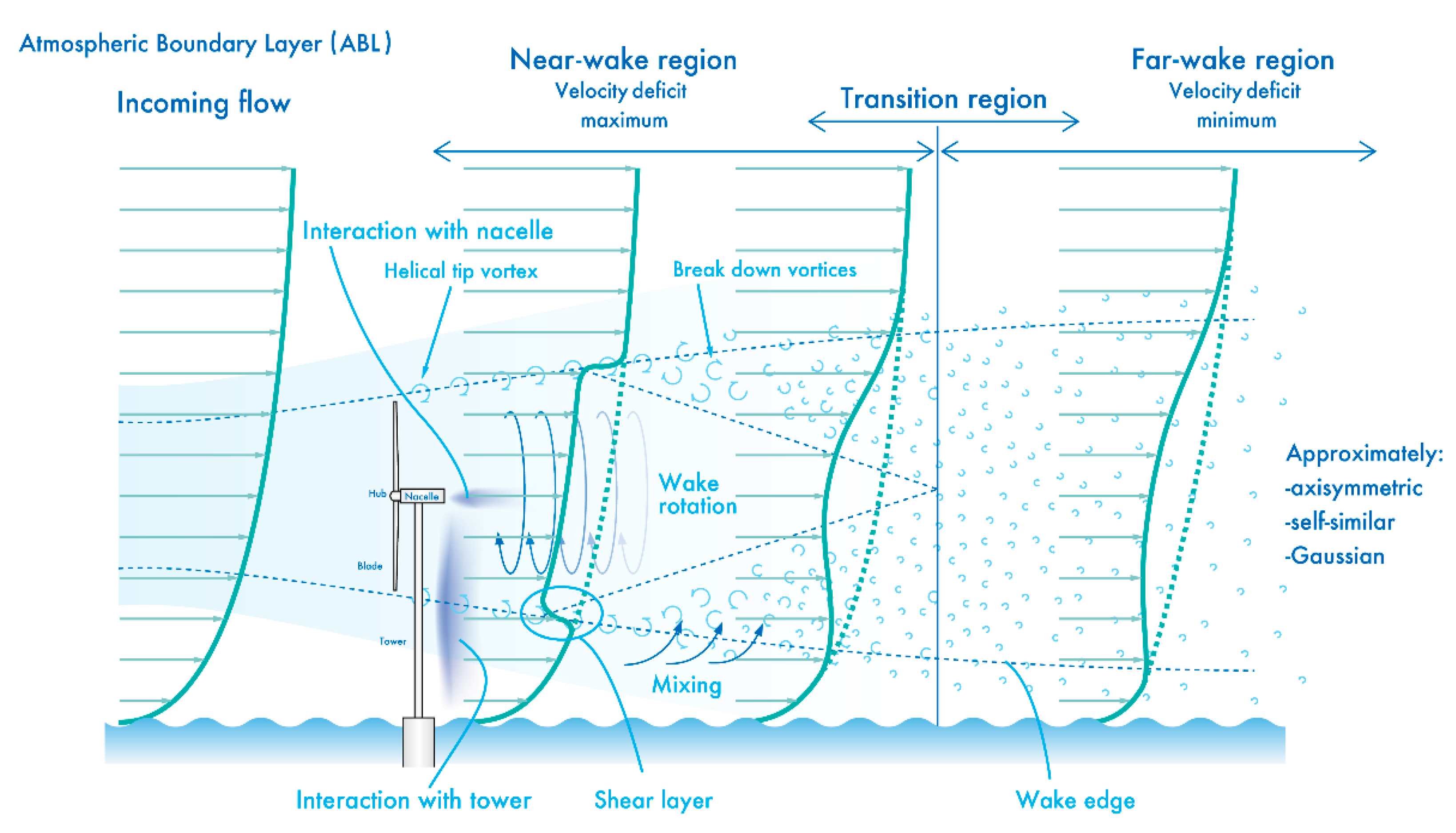
:1. Introduction
2. Wind Measurements of Wind Turbine Near-Wake by Doppler Lidar
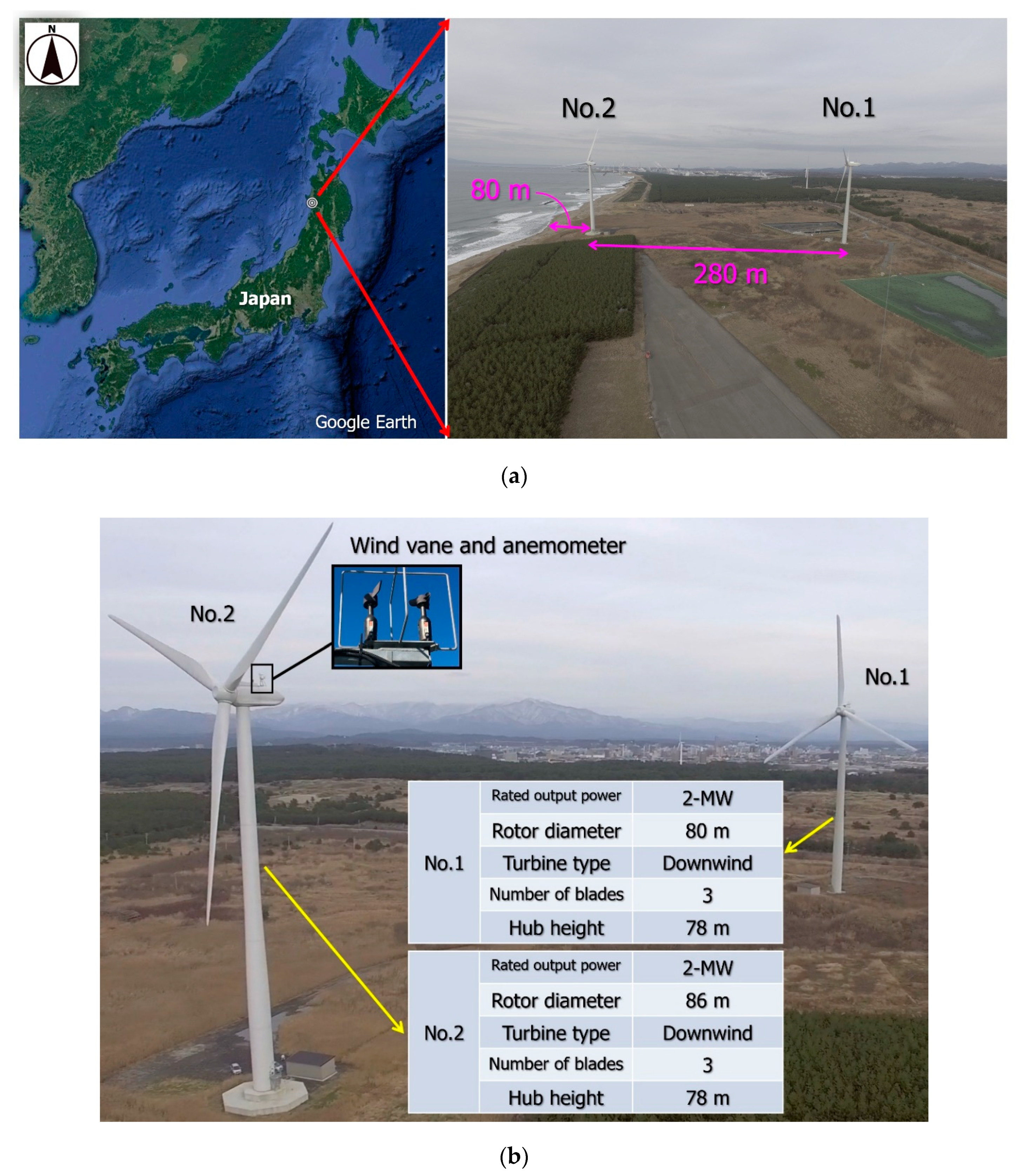
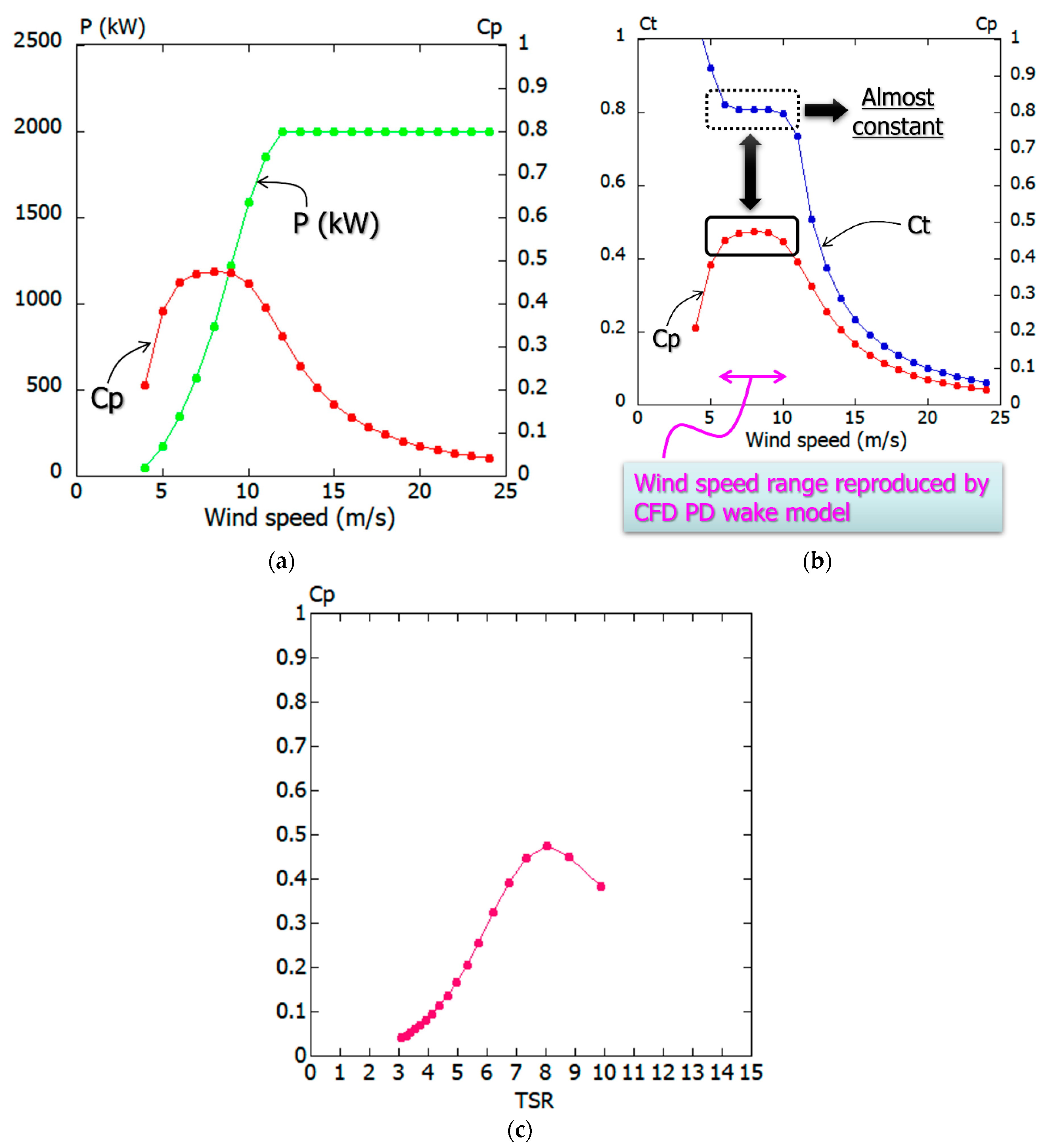
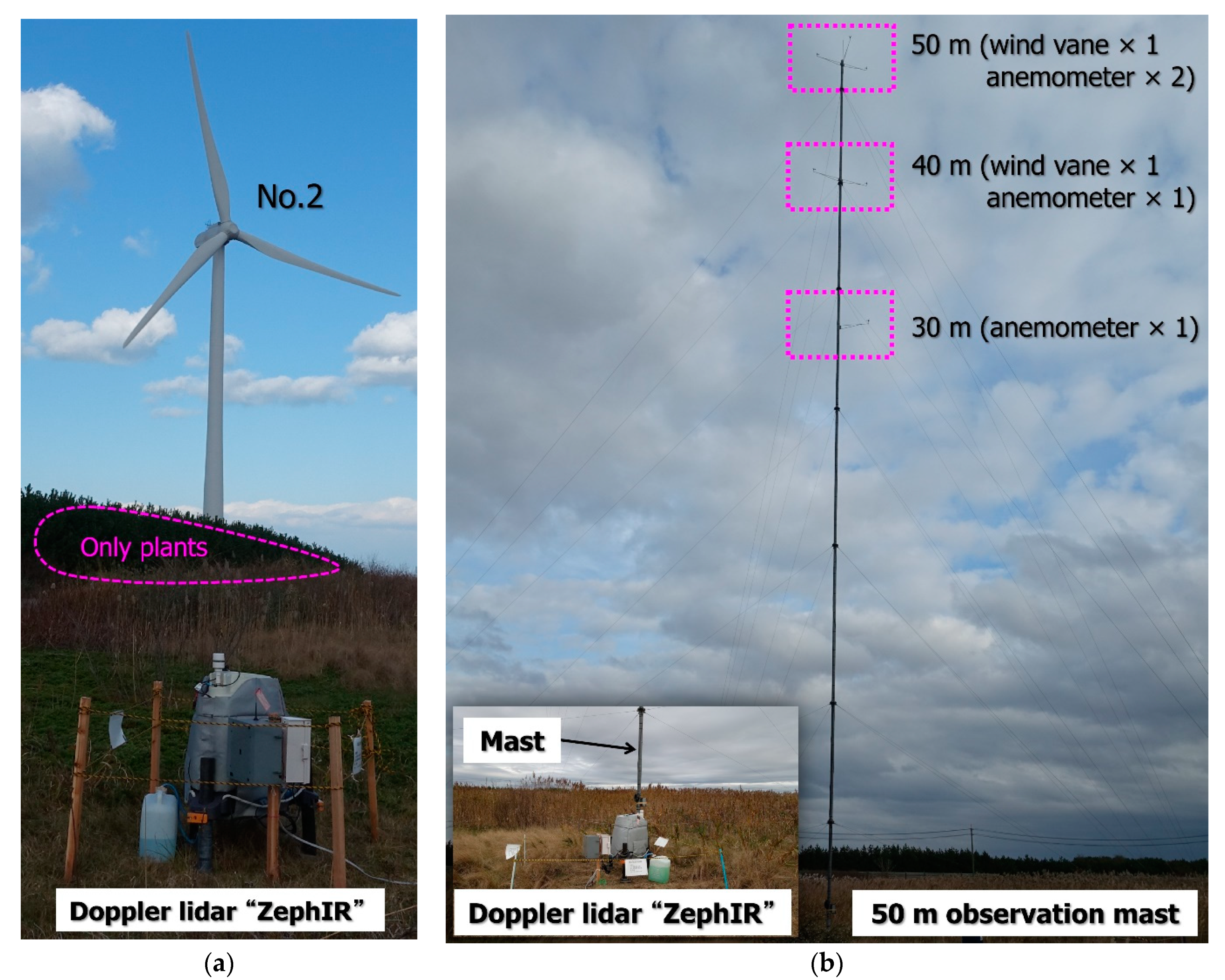
2.1. Overview of Omonogawa Wind Power Station in Akita Prefecture
2.2. Overview of Doppler Lidar Measurement
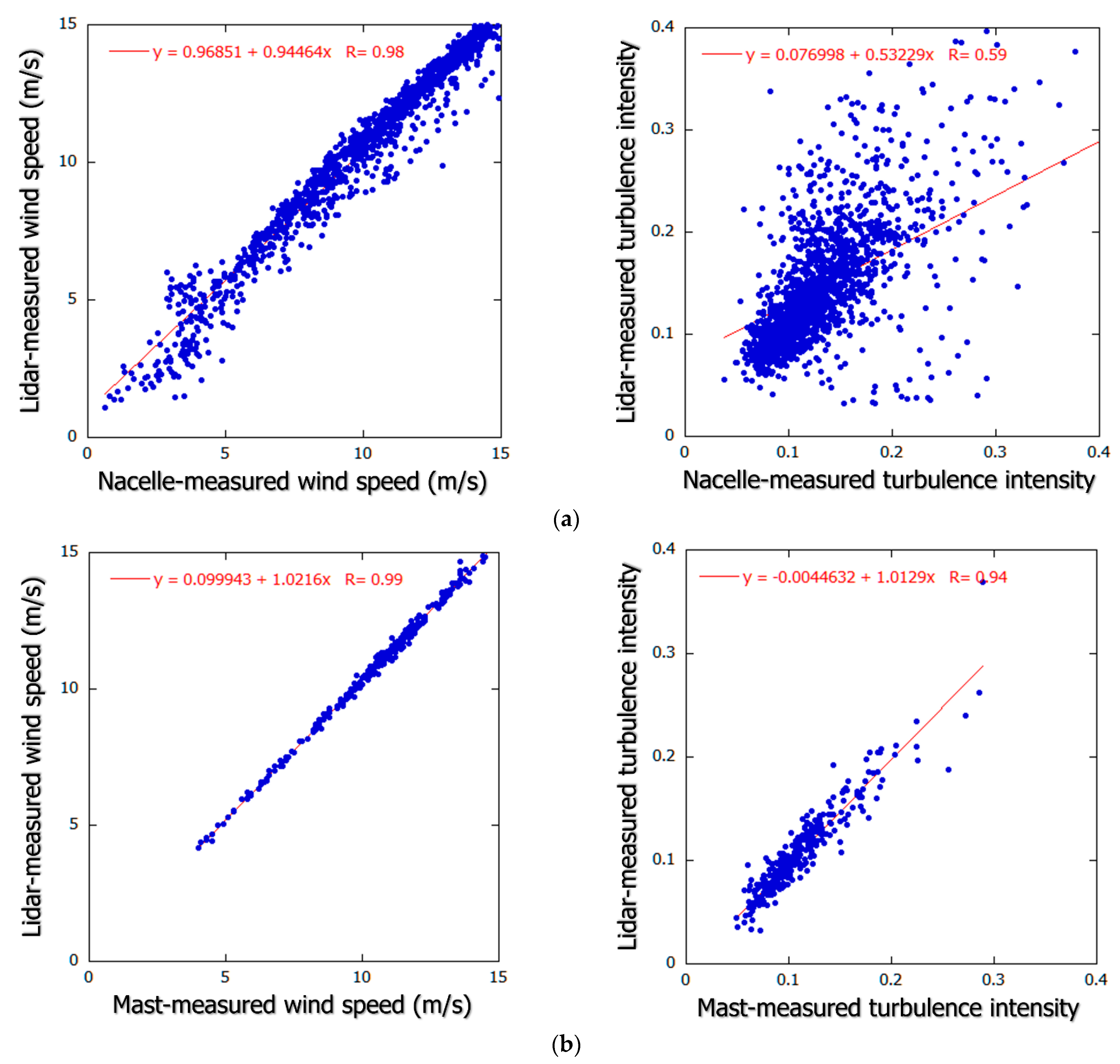
2.3. Verification of Accuracy of Doppler Lidar Measurement
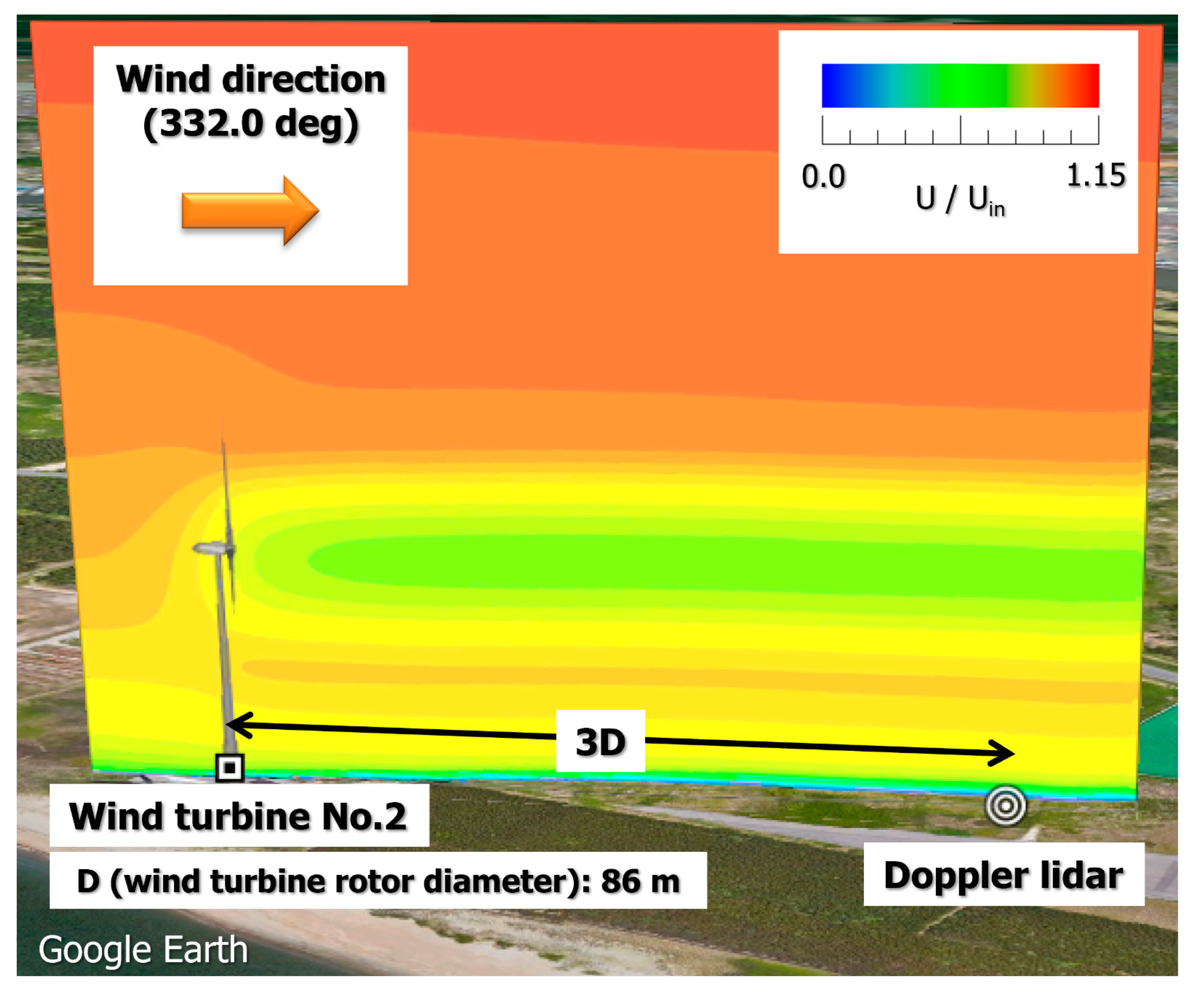
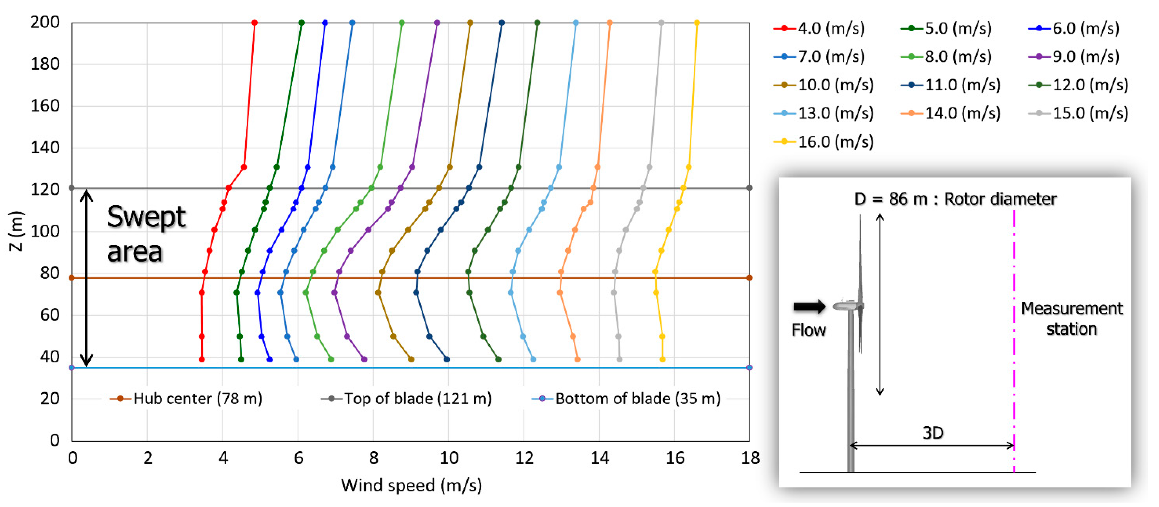
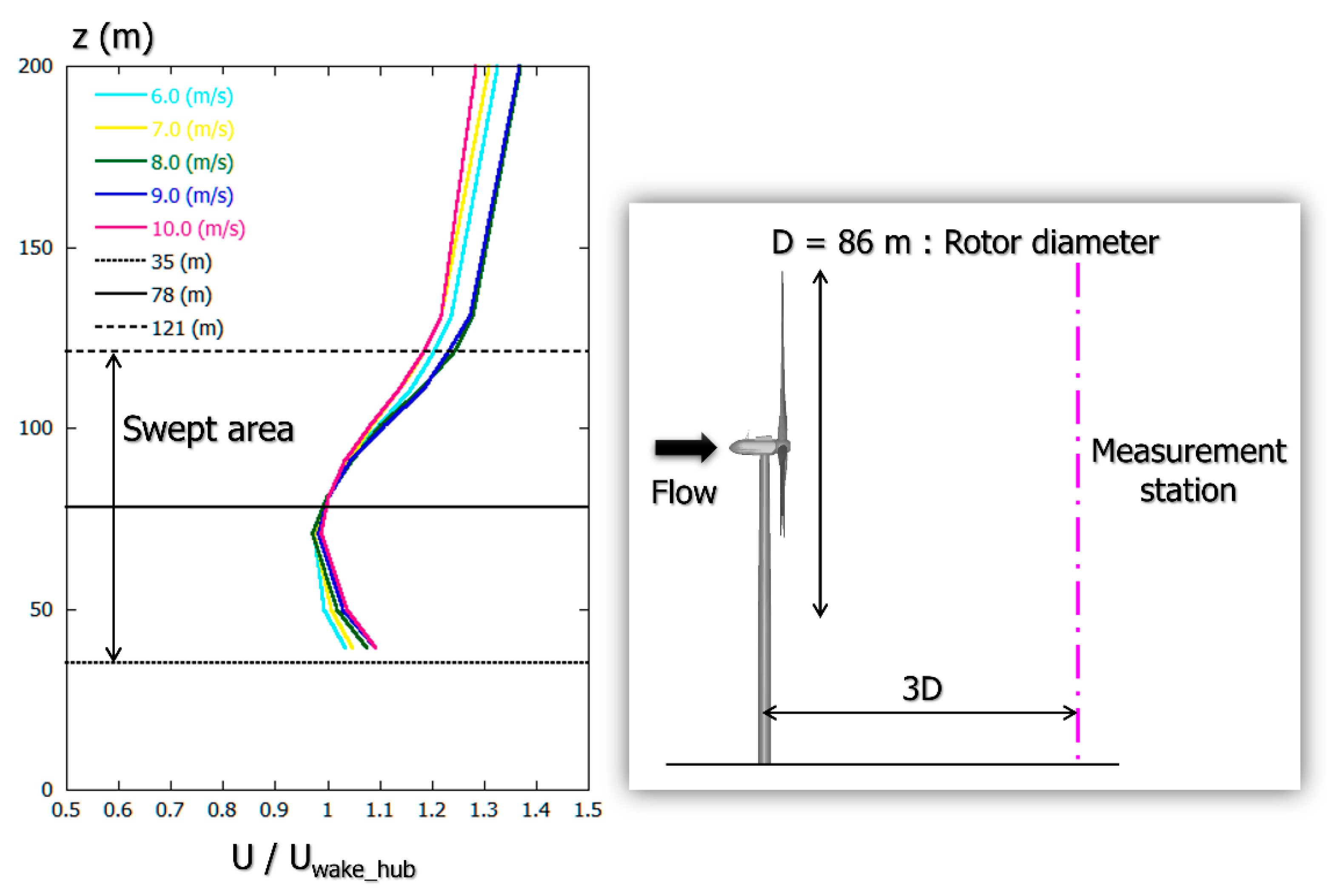
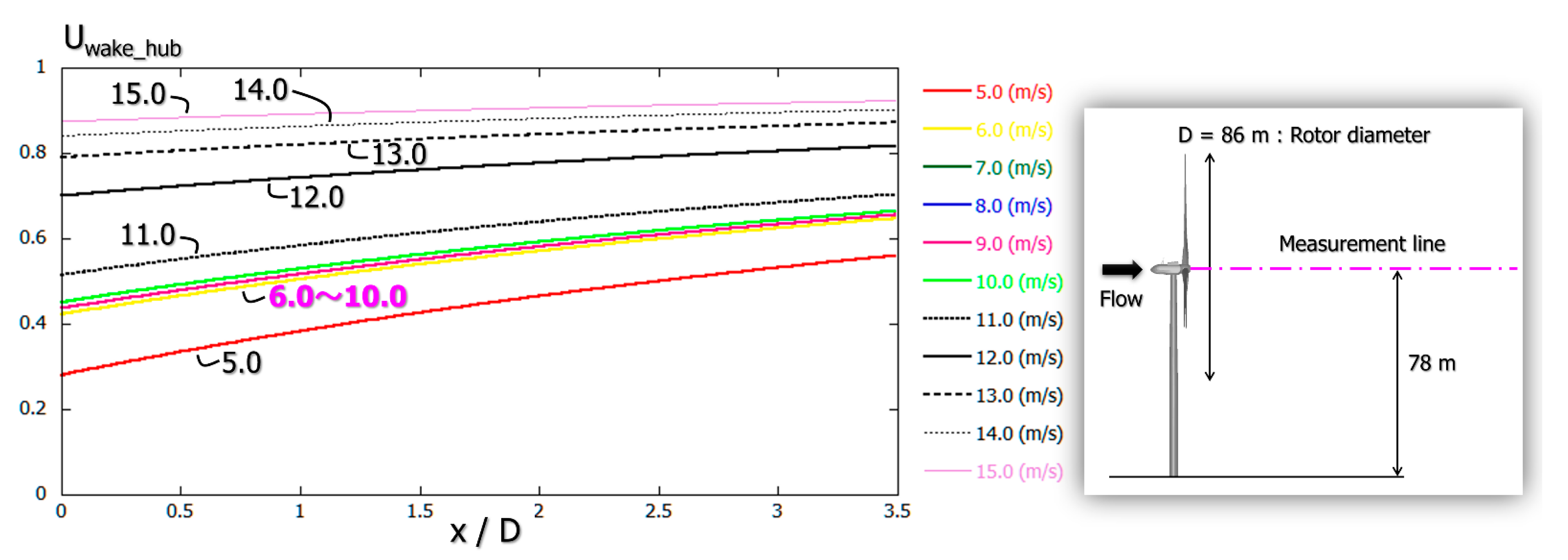
2.4. Doppler Lidar Investigation of Wind Turbine Near-Wakes and Consideration
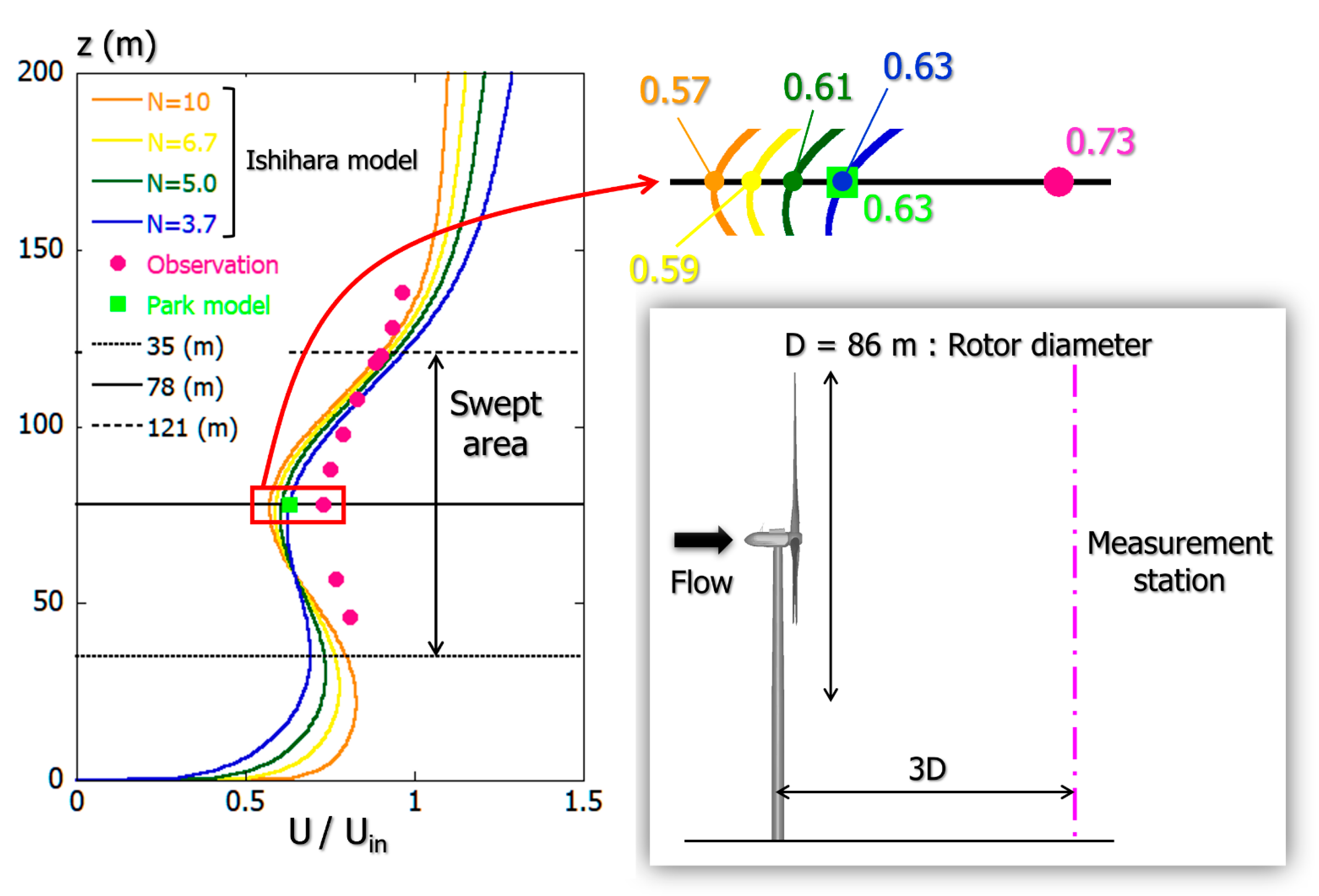
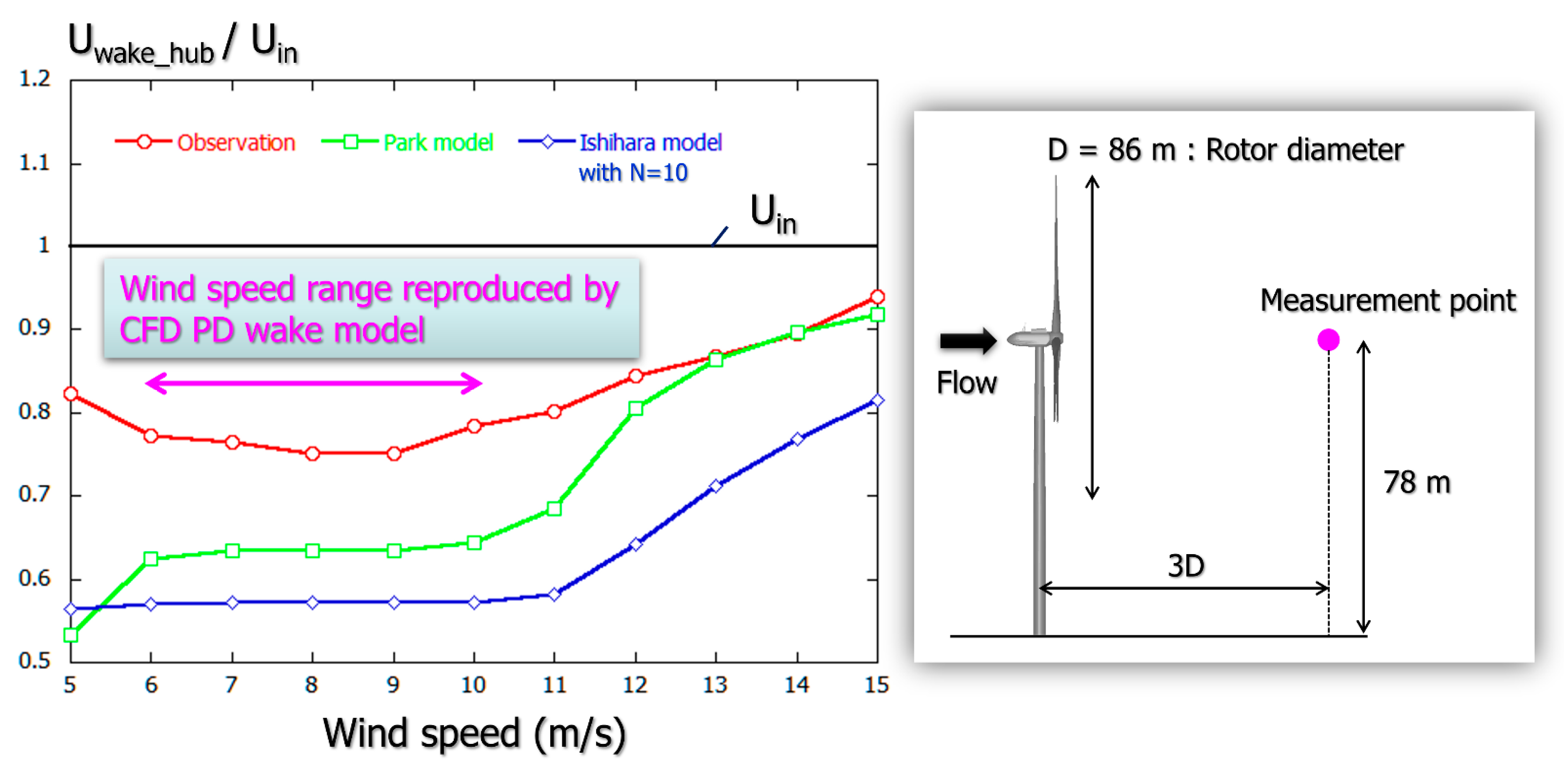
3. Comparison of Wind Measurement Results for Wind Turbine Near-Wake According to Doppler Lidar and Existing Engineering Wake Model
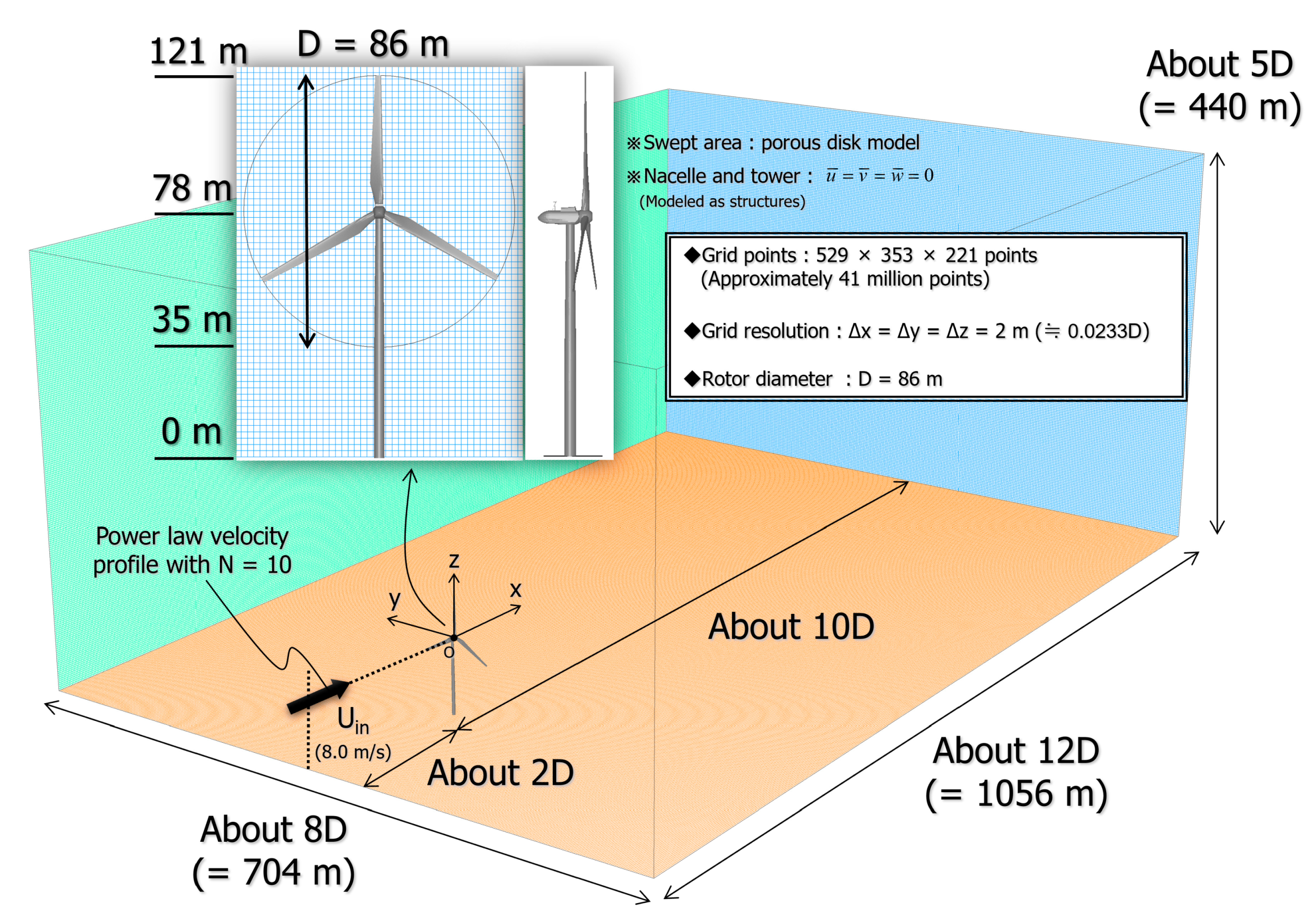
4. CFD Simulations Based on Large Eddy Simulation (LES)
4.1. Overview of LES-Based CFD Approach
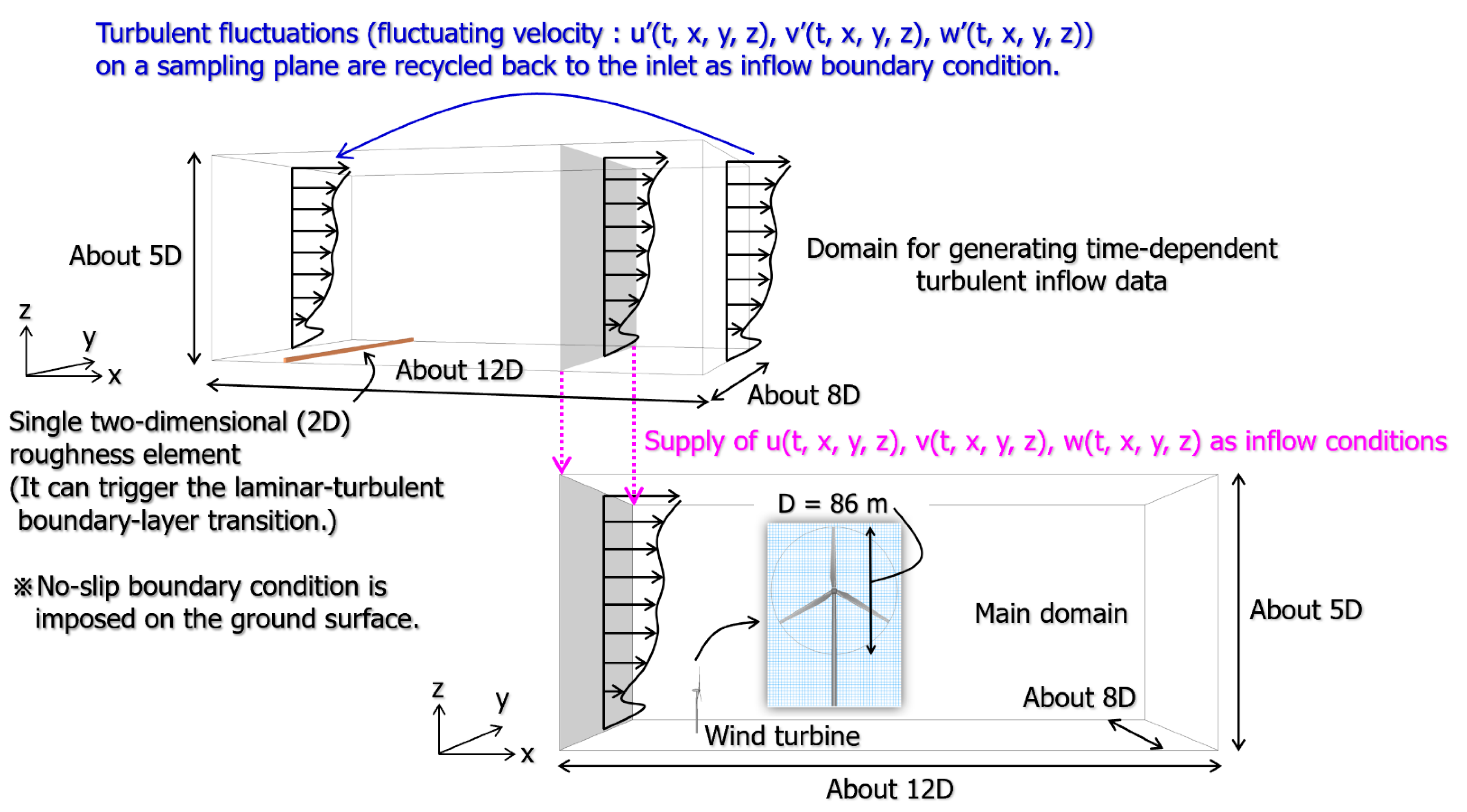
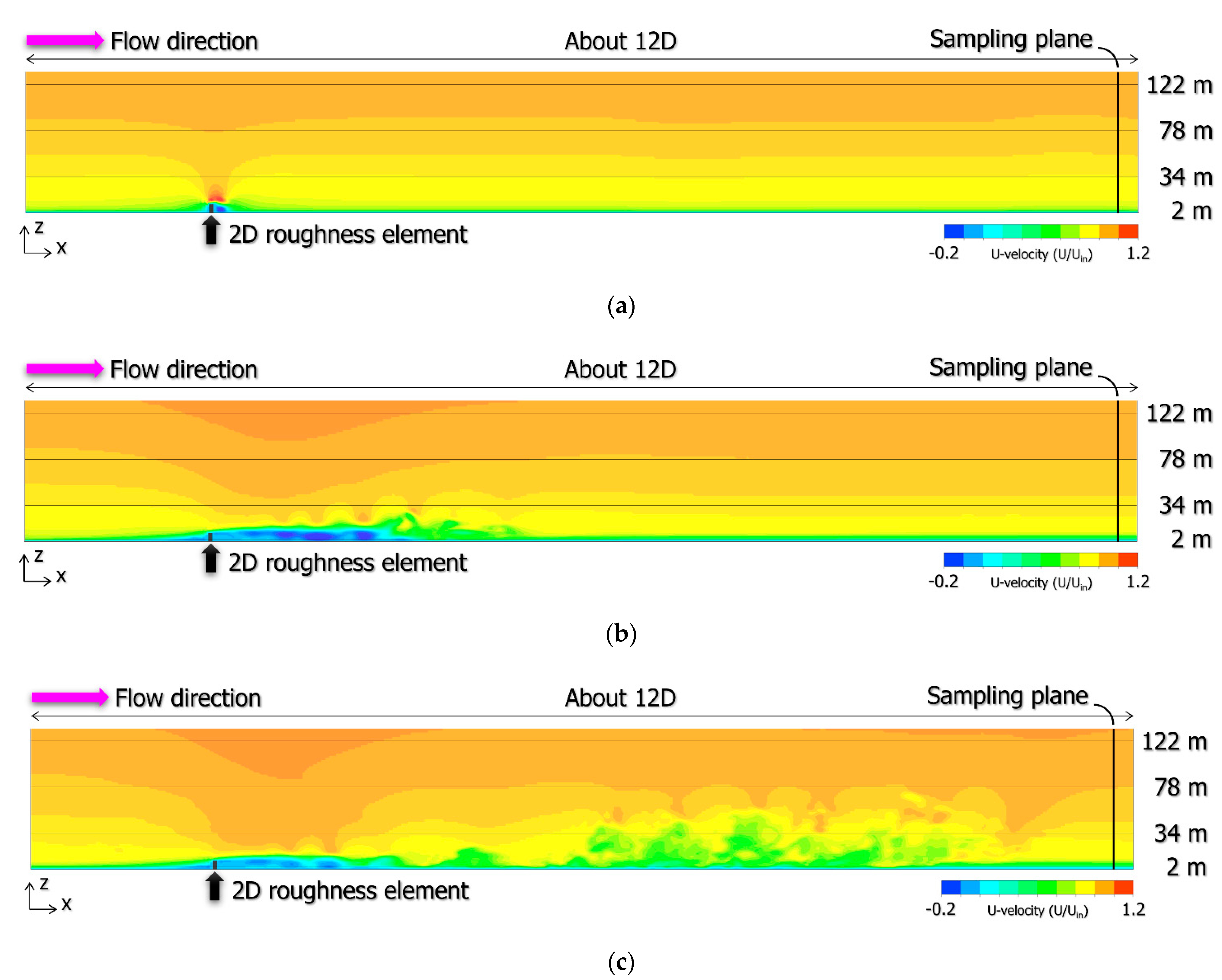
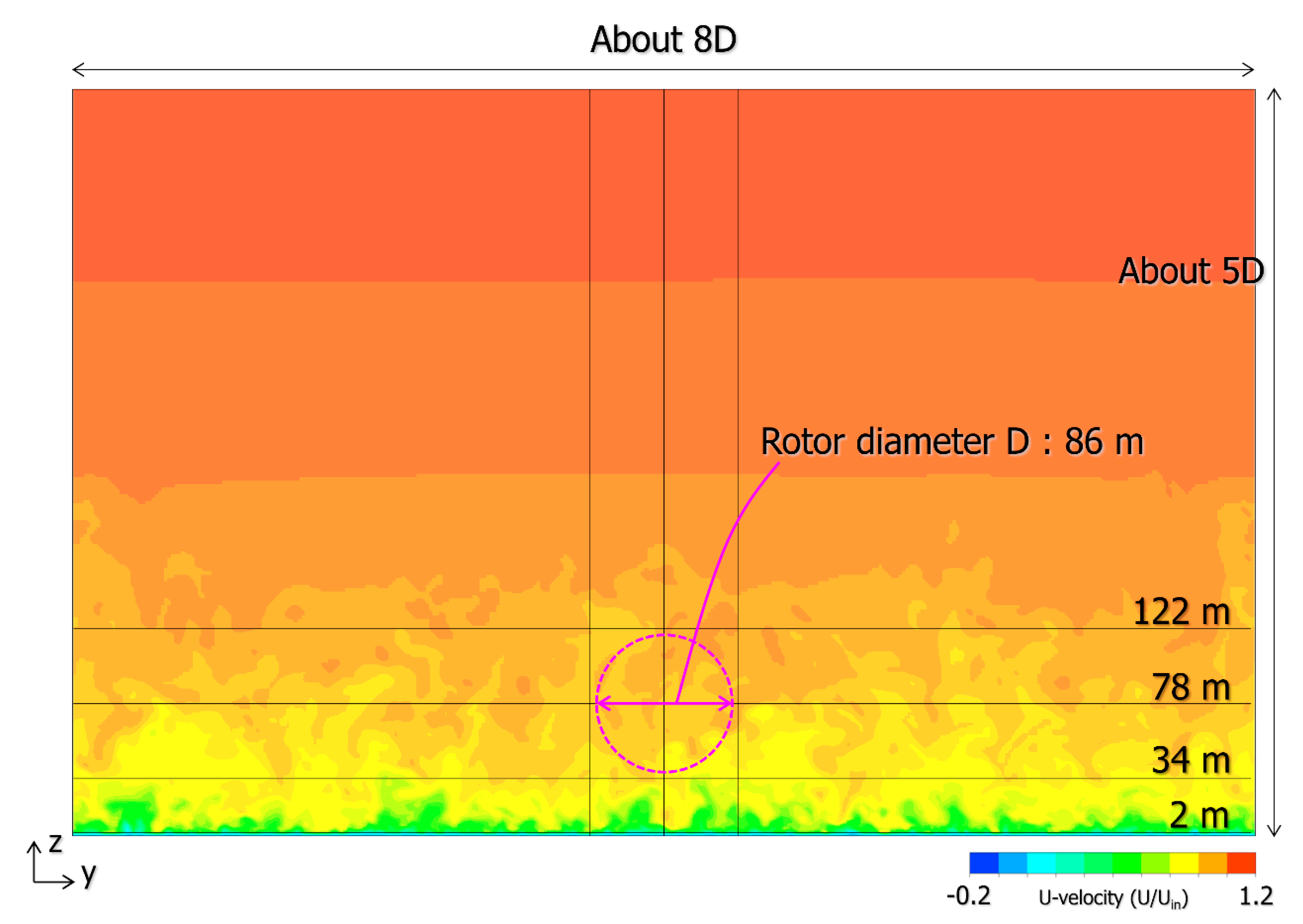
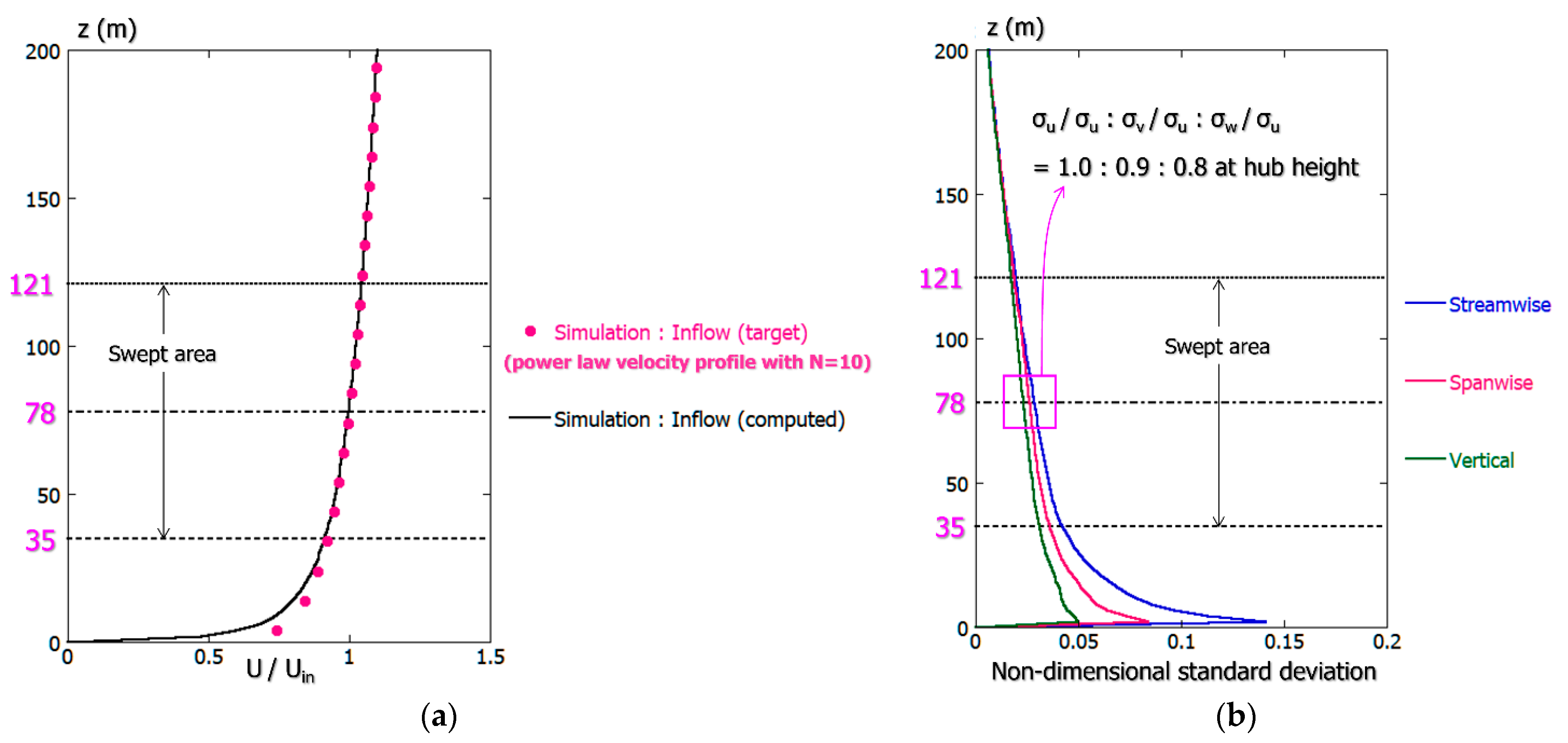
4.2. Inflow Turbulence Generation Methods and Consideration
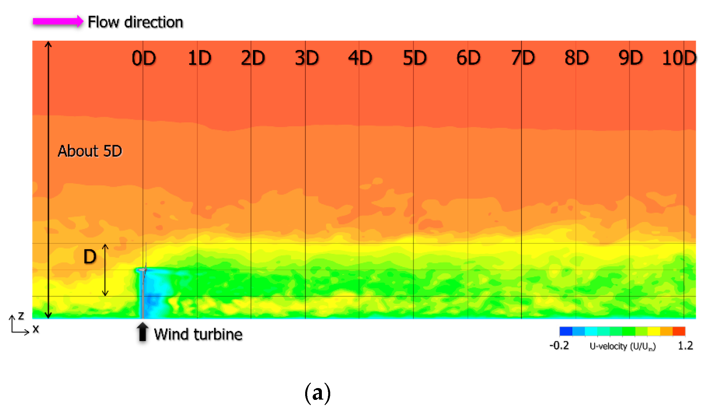
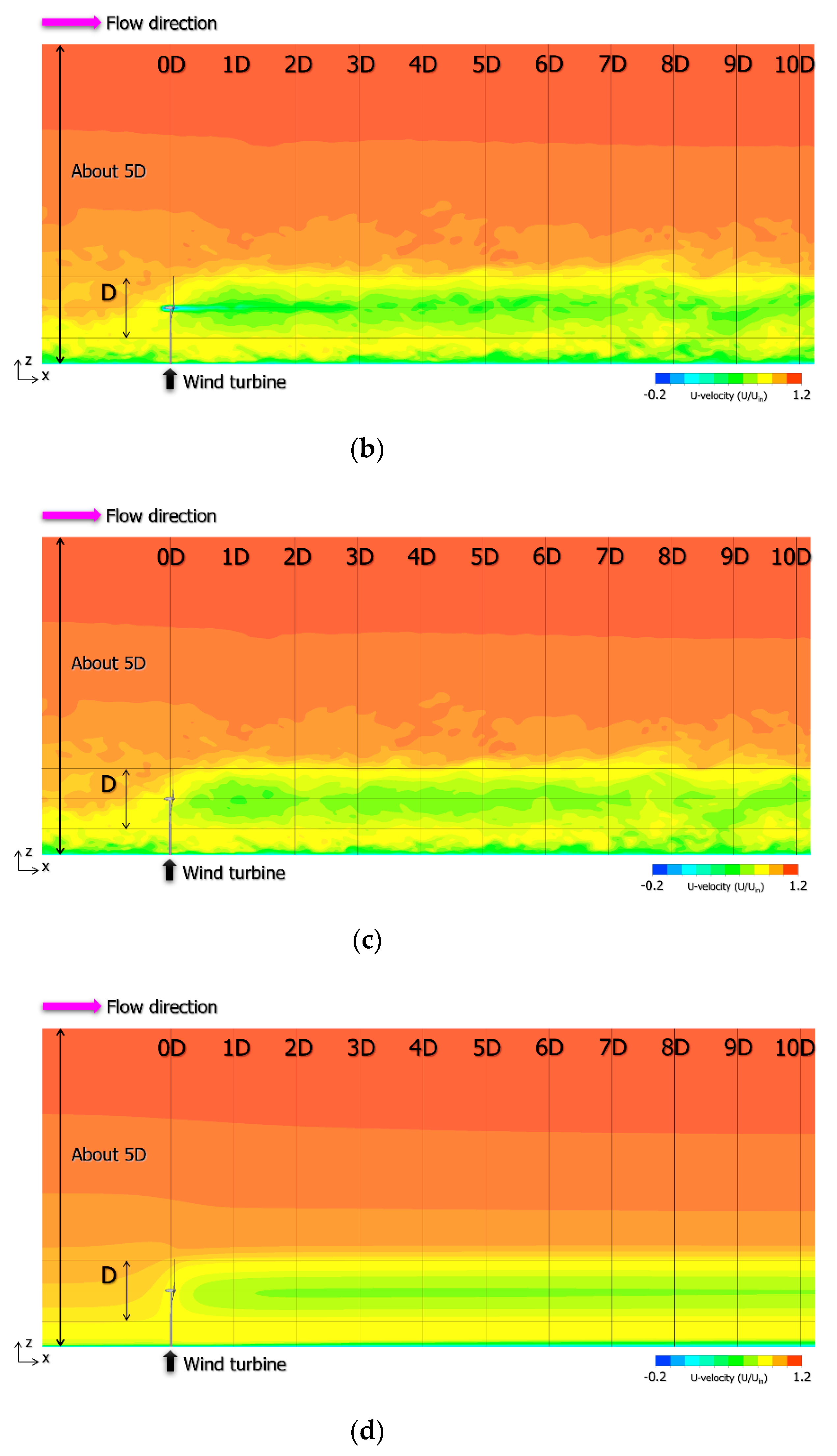
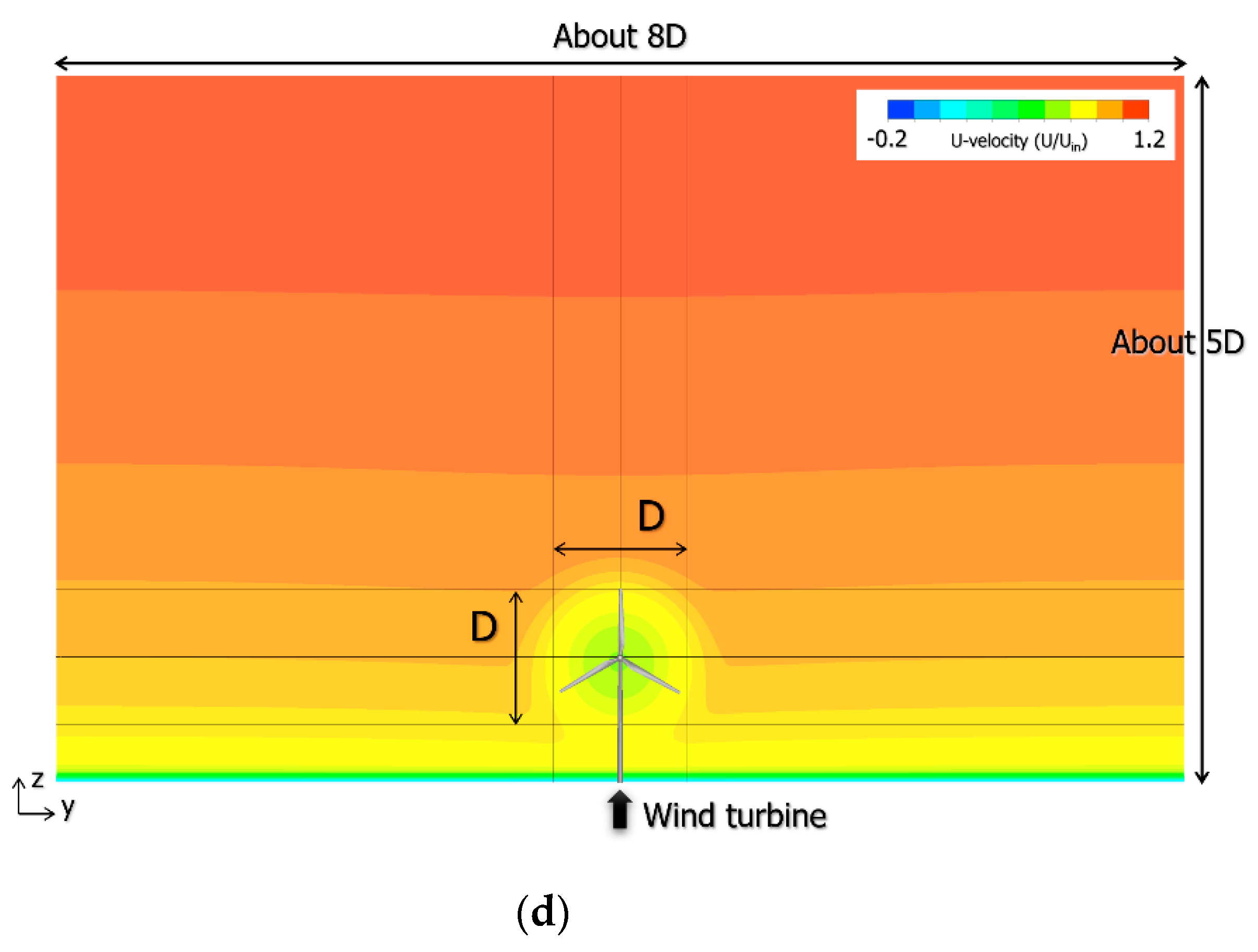
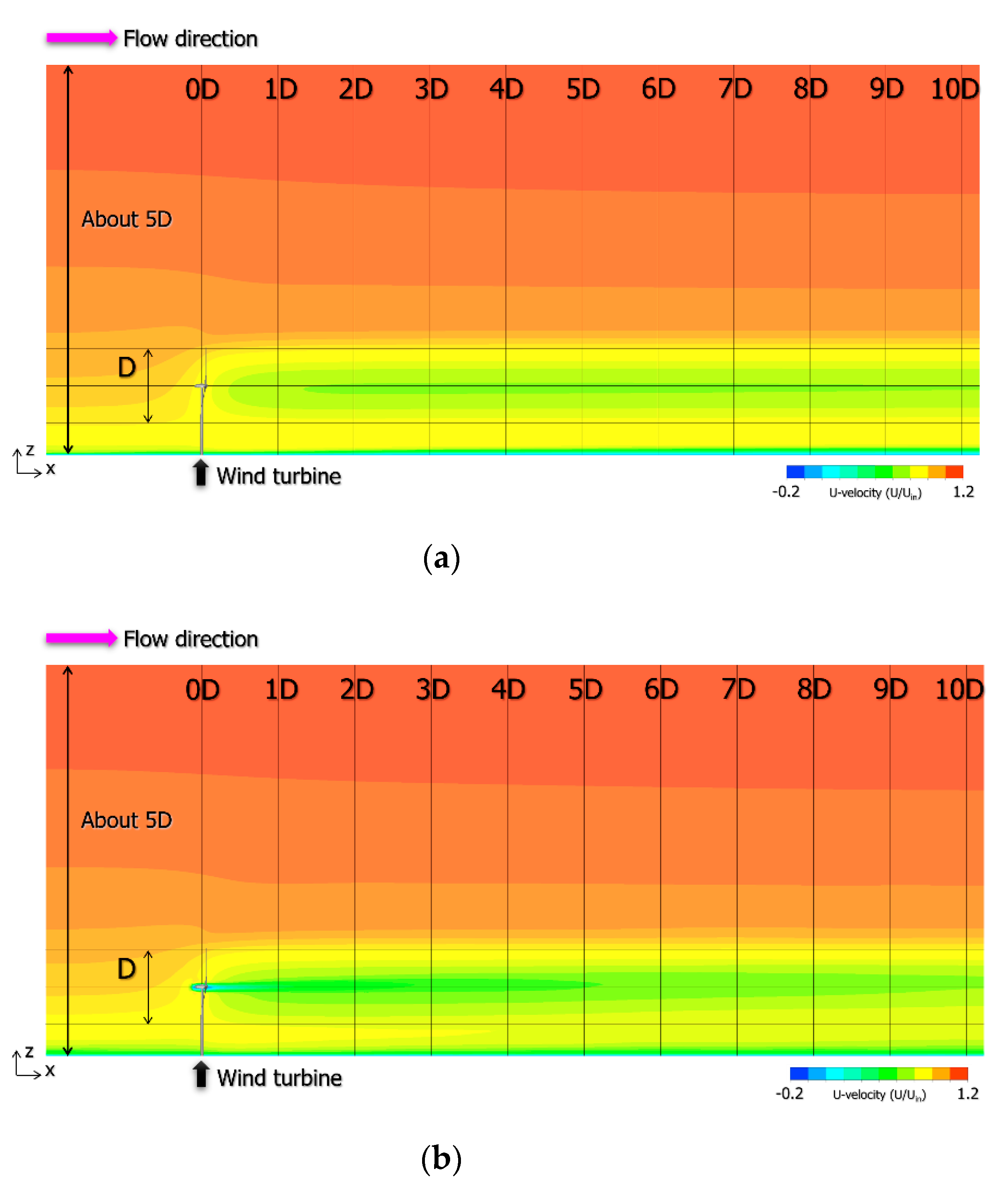
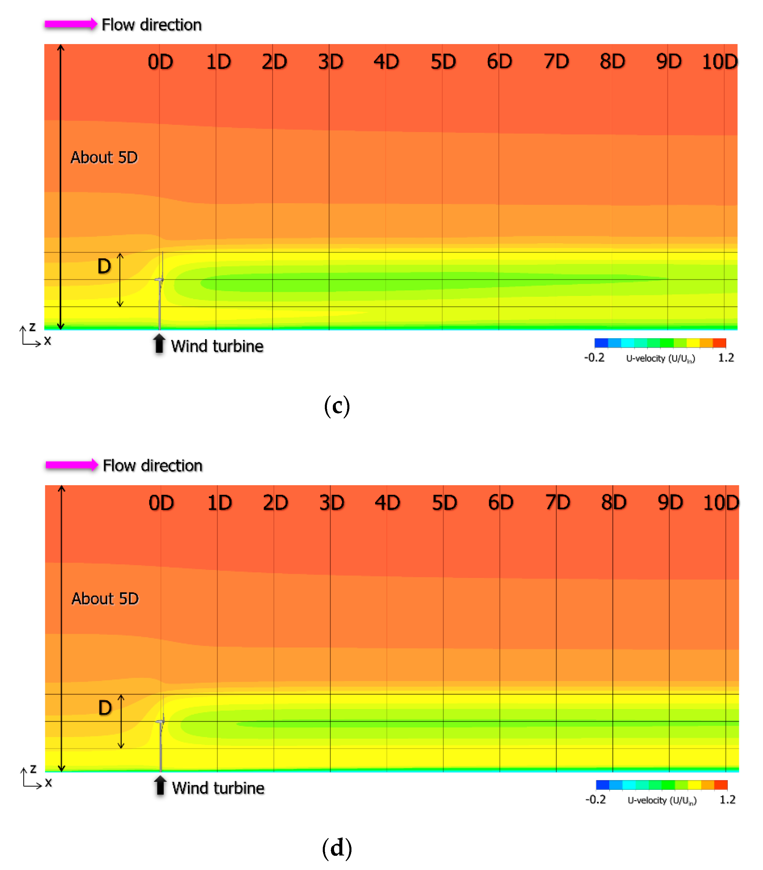
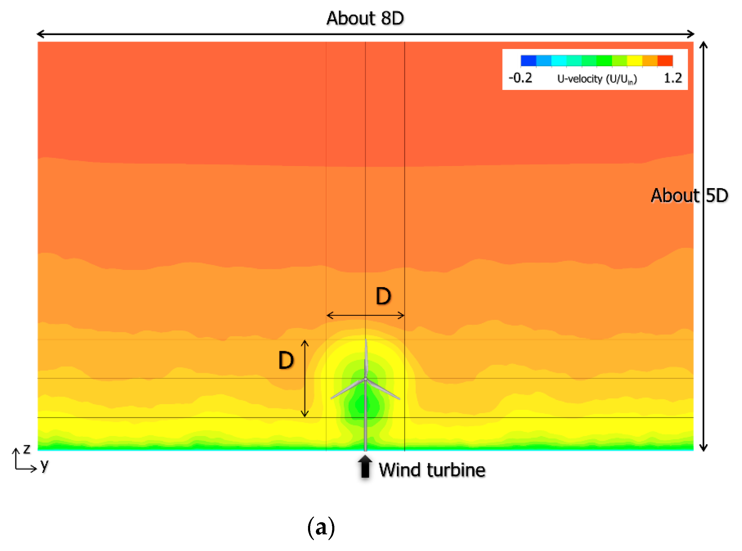
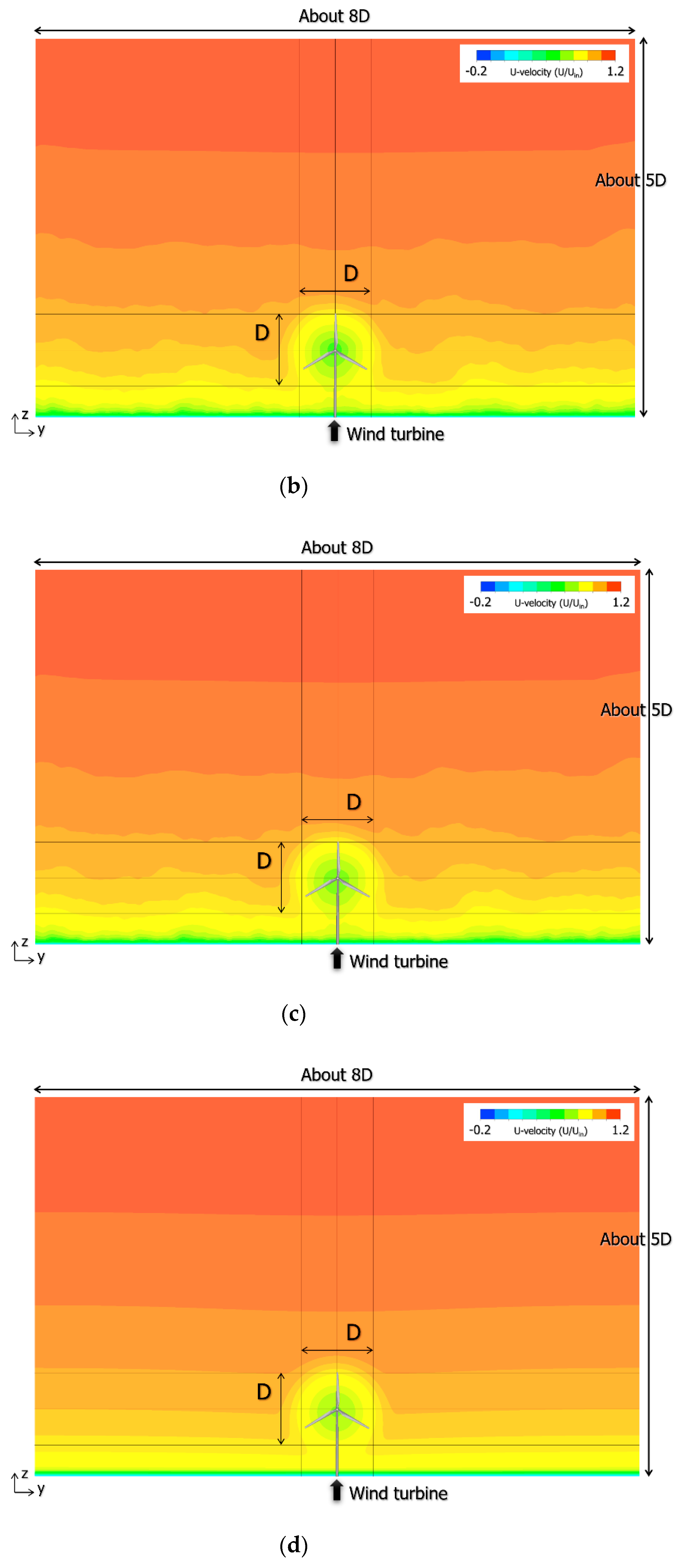
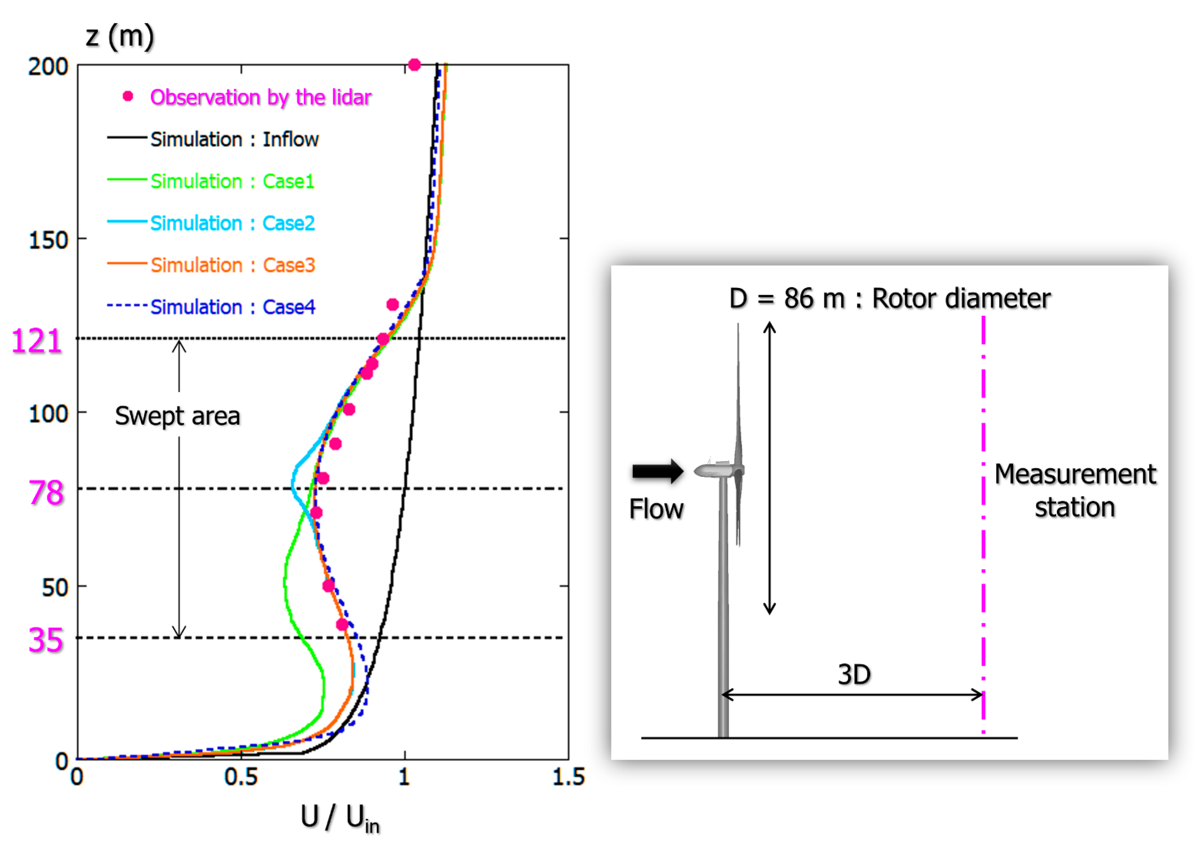
4.3. Large Eddy Simulation (LES) of the Wind Turbine Near-Wake Flow Field Using CFD PD Wake Model and Consideration
5. Conclusions
Author Contributions
Funding
Institutional Review Board Statement
Informed Consent Statement
Data Availability Statement
Acknowledgments
Conflicts of Interest
Appendix A. Arrangement of Park Model Formulation
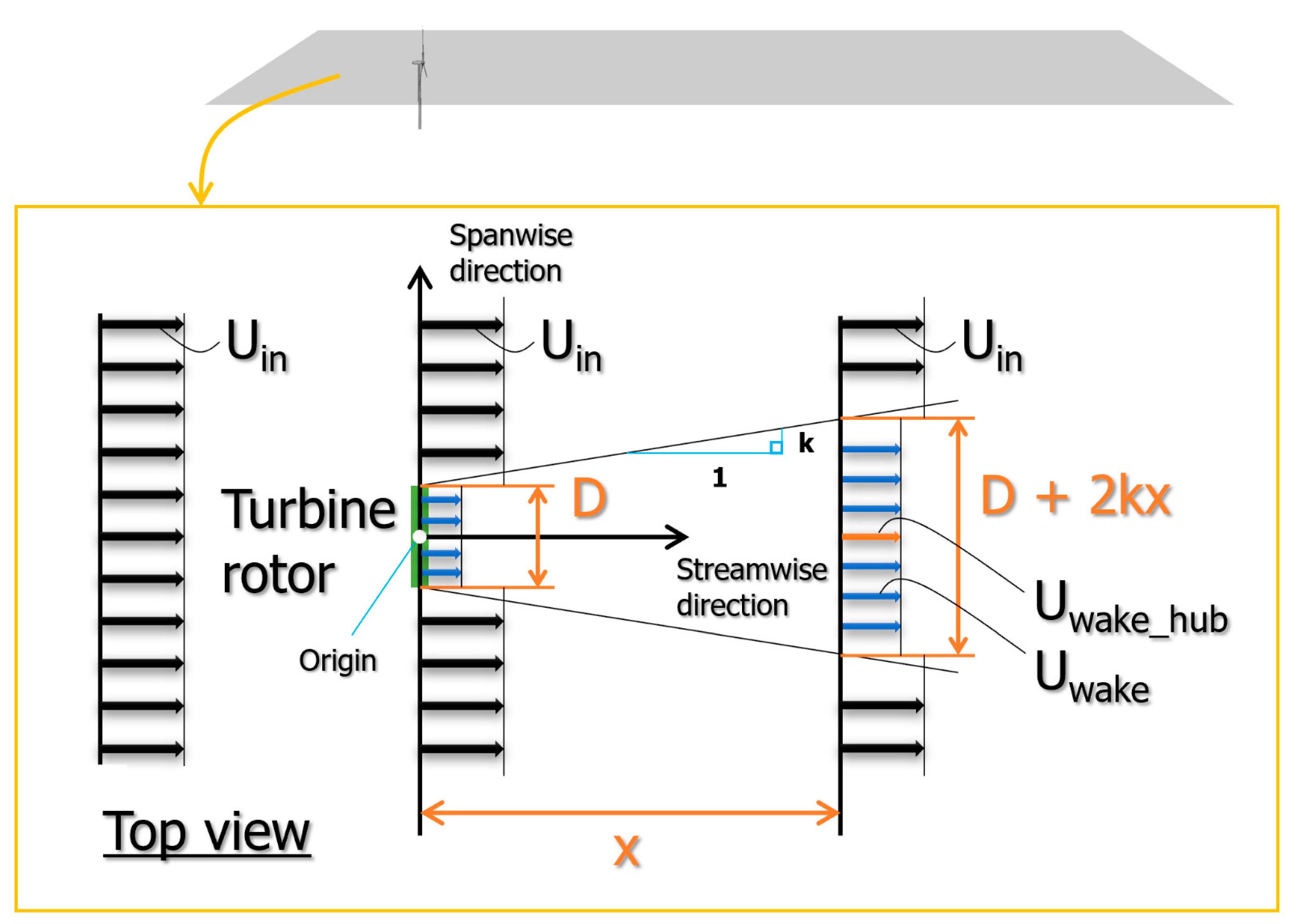
- Uin is the (hub height) inflow wind speed;
- Uwake is the hub height wind speed downstream of the wind turbine at a distance x;
- Ct is the thrust coefficient;
- D is the rotor diameter;
- k is the wake decay constant.
Appendix B. Examination of Effectiveness of Flow Visualization on “Google Earth”
Appendix C. Desktop Study of a Virtual Offshore Wind Farm in the Coastal Area Using the CFD PD Wake Model

References
- Sumner, J.; Watters, C.S.; Masson, C. CFD in Wind Energy: The Virtual, Multiscale Wind Tunnel. Energies 2010, 3, 989–1013. [Google Scholar] [CrossRef] [Green Version]
- Hewitt, S.; Margetts, L.; Revell, A. Building a Digital Wind Farm. Arch. Comput. Methods Eng. 2018, 25, 879–899. [Google Scholar] [CrossRef] [PubMed] [Green Version]
- Porté-Agel, F.; Bastankhah, M.; Shamsoddin, S. Wind-Turbine and Wind-Farm Flows: A Review. Bound. Layer Meteorol 2020, 174, 1–59. [Google Scholar] [CrossRef] [PubMed] [Green Version]
- Dasari, T.; Wu, Y.; Liu, Y.; Hong, J. Near-wake behaviour of a utility-scale wind turbine. J. Fluid Mech. 2019, 859, 204–246. [Google Scholar] [CrossRef]
- Bossuyt, J.; Howland, M.F.; Meneveau, C.; Meyers, J. Measurement of unsteady loading and power output variability in a micro wind farm model in a wind tunnel. Exp. Fluids 2017, 58, 1–17. [Google Scholar] [CrossRef] [Green Version]
- Ansys CFX. Turbomachinery CFD Software. Available online: https://www.ansys.com/products/fluids/ansys-cfx (accessed on 1 March 2020).
- Simcenter STAR-CCM+. Available online: https://www.plm.automation.siemens.com/global/de/products/simcenter/STAR-CCM.html (accessed on 1 March 2020).
- Jensen, N.O. A Note on Wind Generator Interaction; Technical Report Risoe-M-2411(EN); Risø National Laboratory: Roskilde, Denmark, 1983. [Google Scholar]
- Katic, I.; Højstrup, J.; Jensen, N.O. A simple model for cluster efficiency. In Proceedings of the European Wind Energy Association Conference & Exhibition (EWEC’86), Rome, Italy, 6–8 October 1986; Volume 1, pp. 407–410. [Google Scholar]
- Uchida, T.; Taniyama, Y.; Fukatani, Y.; Nakano, M.; Bai, Z.; Yoshida, T.; Inui, M. A New Wind Turbine CFD Modeling Method Based on a Porous Disk Approach for Practical Wind Farm Design. Energies 2020, 13, 3197. [Google Scholar] [CrossRef]
- Scientific, C. Finance Grade Performance, ZephIR 300; Technical Report; Campbell Scientific, Inc.: Edmonton, AB, Canada, 2016. [Google Scholar]
- Kogaki, T.; Sakurai, K.; Shimada, S.; Kawabata, H.; Otake, Y.; Kondo, K.; Fujita, E. Field Measurements of Wind Characteristics Using LiDAR on a Wind Farm with Downwind Turbines Installed in a Complex Terrain Region. Energies 2020, 13, 5135. [Google Scholar] [CrossRef]
- Ishihara, T.; Qian, G. Numerical and Analytical Study of Wind Turbine Wakes. In Proceedings of the National Symposium on Wind Engineering, Tokyo, Japan, 5–7 December 2016; Volume 24, pp. 151–156. [Google Scholar]
- Uchida, T.; Araya, R. Practical Applications of the Large-Eddy Simulation Technique for Wind Environment Assessment around New National Stadium, Japan (Tokyo Olympic Stadium). Open J. Fluid Dyn. 2019, 9, 269. [Google Scholar] [CrossRef] [Green Version]
- Inagaki, M.; Kondoh, T.; Nagano, Y. A Mixed-Time-Scale SGS Model with Fixed Model-Parameters for Practical LES. ASME J. Fluids Eng. 2005, 127, 1–13. [Google Scholar] [CrossRef]
- Uchida, T.; Kawashima, Y. New Assessment Scales for Evaluating the Degree of Risk of Wind Turbine Blade Damage Caused by Terrain-Induced Turbulence. Energies 2019, 12, 2624. [Google Scholar] [CrossRef] [Green Version]
- Uchida, T.; Takakuwa, S. A Large-Eddy Simulation-Based Assessment of the Risk of Wind Turbine Failures Due to Terrain-Induced Turbulence over a Wind Farm in Complex Terrain. Energies 2019, 12, 1925. [Google Scholar] [CrossRef] [Green Version]
- Lund, T.S.; Wu, X.; Squires, K.D. Generation of Turbulent Inflow Data for Spatially-Developing Boundary Layer Simulations. J. Comput. Phys. 1998, 140, 233–258. [Google Scholar] [CrossRef] [Green Version]


| Wind Speed (m/s) | 4 | 5 | 6 | 7 | 8 | 9 | 10 | 11 | 12 | 13 | 14 | 15 | 16 |
|---|---|---|---|---|---|---|---|---|---|---|---|---|---|
| Number | 5 | 13 | 28 | 36 | 25 | 31 | 43 | 36 | 31 | 31 | 22 | 11 | 6 |
| Case 1 | Case 2 | Case 3 | Case 4 | |
|---|---|---|---|---|
| Blade (swept area): CFD PD wake model (CRC = 2.5) | ○ | |||
| Nacelle: body ※ | ○ | ○ | × | × |
| Tower: body ※ | ○ | × | × | × |
| Inflow turbulence | ○ | × | ||
Publisher’s Note: MDPI stays neutral with regard to jurisdictional claims in published maps and institutional affiliations. |
© 2021 by the authors. Licensee MDPI, Basel, Switzerland. This article is an open access article distributed under the terms and conditions of the Creative Commons Attribution (CC BY) license (https://creativecommons.org/licenses/by/4.0/).
Share and Cite
Uchida, T.; Yoshida, T.; Inui, M.; Taniyama, Y. Doppler Lidar Investigations of Wind Turbine Near-Wakes and LES Modeling with New Porous Disc Approach. Energies 2021, 14, 2101. https://doi.org/10.3390/en14082101
Uchida T, Yoshida T, Inui M, Taniyama Y. Doppler Lidar Investigations of Wind Turbine Near-Wakes and LES Modeling with New Porous Disc Approach. Energies. 2021; 14(8):2101. https://doi.org/10.3390/en14082101
Chicago/Turabian StyleUchida, Takanori, Tadasuke Yoshida, Masaki Inui, and Yoshihiro Taniyama. 2021. "Doppler Lidar Investigations of Wind Turbine Near-Wakes and LES Modeling with New Porous Disc Approach" Energies 14, no. 8: 2101. https://doi.org/10.3390/en14082101