
Solar Radiation on a Parabolic Concave Surface


School of Electrical Engineering, Tel Aviv University, Tel Aviv 699768, Israel
*
Author to whom correspondence should be addressed.
Energies 2021, 14(8), 2245; https://doi.org/10.3390/en14082245
Submission received: 24 February 2021
/
Revised: 5 April 2021
/
Accepted: 13 April 2021
/
Published: 16 April 2021
Abstract
:Curved structures are used in buildings and may be integrated with photovoltaic modules. Self-shading occurs on non-flat (curved) surface collectors resulting in a non-uniform distribution of the direct beam and the diffuse incident solar radiation along the curvature the surface. The present study uses analytical expressions for calculating and analyzing the incident solar radiation on a general parabolic concave surface. Concave surfaces facing north, south and east/west are considered, and numerical values for the annual incident irradiations (in ) are demonstrated for two locations: (Tel Aviv, Israel) and (Lindenberg, Germany). The numerical results show that the difference in the incident global irradiation for the different surface orientations is not very wide. At , the irradiation difference between the south and north-oriented surface is about 15 percent, and between the south and east surface orientation it is about 9.6 percent. For latitude , the global irradiation difference between the south and north-oriented surface is about 16 percent, and between the south and east orientation it is about 3 percent.

1. Introduction
Curved structures with concave and convex surfaces are used in buildings and may be integrated with photovoltaic (PV) modules (known as BIPV) to generate electrical power. PV modules on curved surfaces are self-shading, negatively affecting the generated power. In addition, the direct beam and the diffuse incident radiation are not uniform distributed along the curvature of the surfaces because the slope of the surface varies with the distance. Concave structures (e.g., canopies, facades, overhangs) have elegant curvatures that enhance the aesthetics of the building and may be covered with flexible PV modules to generate electricity. Solar radiation on a catenary collector was first published in [1,2] for an exploration mission to Mars. Years later, photovoltaic collectors on a convex surface were analyzed with respect to self-shading and incident solar radiation [3]. A few publications on solar systems with curved surfaces are mentioned in [4,5,6,7,8] presenting results but not analytical derivations, except reference [4] which forms analytically (by Bézier curve used in computer graphics) the surface curvature by many small triangular flat pieces. A solar thermal collector of a quarter cylindrical shape is proposed in [5], and a method that approximates a double-curved surface by using flat strips deployed on curved surface is in [6]. A publication on interconnecting PV modules mounted on a curvature surface to minimize the self-shading effect is in [7]. Representing a curved surface by flat segments is suggested again in [8]. Self-shading on curved surface was first addressed in [1] for a catenary shape surface and for a convex shape surface in [3]. The analytical expressions for self-shading development in the present work follow the methodology in [1,3]. Reference [1] deals mainly with self-shading on a catenary surface deployed on a Martian surface, and some results of solar radiation are presented. Reference [3] deals, however, with self-shading and solar radiation calculations on a convex surface relevant to Earth. The present work compliments and adds to the work in [3] by dealing with a concave surface; thus, both studies cover curved surfaces that may be used in buildings and in other structures such greenhouses. References [4,5,6,7,8] do not deal with self-shading, an important effect to consider in solar radiation calculation on curved surfaces, which consequently affects the electrical energy generated by the PV modules. Self-shading on a PV collector results in shading a part of the collector and the remaining part receives solar radiation. The pattern and dimensions of these parts varies with time according to the sun position in the sky. The present paper develops analytical expressions for calculating the self-shading areas, direct beam, diffuse and global incident radiation on a (smooth) parabolic concave PV collector that is applicable to BIPV. Concave surfaces facing north, south and east/west are considered, and numerical values of the annual incident irradiations (in ) are demonstrated for two locations: (Tel Aviv, Israel) and (Lindenberg, Germany). The calculation shows that the south-oriented surface receives the highest irradiation, next is the east surface and last is the north surface; however, the difference in the irradiation is not very big and is about 15 percent between the south and north-oriented parabolic surfaces.
2. Materials and Methods
Self-shading occurs on curved surfaces. To determine the state of shading and the incident solar radiation, a parabolic concave surface is chosen and analyzed with respect to the surface orientation toward the north, south and east/west. The patterns and dimensions of the shading, which vary with time according to the sun’s position in the sky, are formulated to obtain the incident solar radiation on the different surfaces.
2.1. Concave Parabolic Surface Equation
Given a concave surface of the form (see Figure 1),
The coefficients and are determined by the concave surface parameters and , implying
and the surface equation becomes
The derivative of Equation (3) is
2.2. Self-Shading in a Concave Parabolic Surface-North Facing
The derivation of the shading, in the present article, pertains to a concave parabolic surface deployed in the northern hemisphere. Self-shading occurs when the sun is behind the surface. At locations with latitudes higher than , for south-facing surfaces this happens only in summer at times when the sun azimuth, in absolute terms, is greater than . For north facing surfaces, self-shading may occur during any time in the year, depending on the geographical location and on the concave surface dimensions. For an arbitrarily oriented collector, self-shading appears for longer periods. A concave collector (see Figure 1) is self-shading; the pattern and size of the shaded and unshaded areas depend on the sun’s position in the sky. To determine the shape and area of the shadow, a north-facing collector is first considered (see Figure 1). The results for an arbitrary oriented surface may be generalized by replacing the sun’s azimuth angle with ,
where is the surface azimuth angle with respect to the south.
Figure 2 shows the shadow components and of a line of the concave surface. The components are given by
where is the sun’s altitude.
The condition for is either case (ii) or case (iii), according to the following:
For corresponds to case (ii),
For corresponds to case (iii).
Case (i) is shown in Figure 3 indicating the shaded area in grey and the exposed area to sun’s rays is in white.
The coordinates of points and are given in [1] Appendix B.
Case (i):
Case (ii):
Case (iii):
2.3. States of Shading
To illustrate the shading effect on a concave collector at different times during the year, the following dimensions of a parabolic surface are used as an example: .
The parabolic equation and the derivative become the following (see Equations (3) and (4)):
The state of shading depends on the surface dimensions and on the latitude location represented by the sun’s altitude and the sun’s azimuth on different hours and dates. The well-known relations for and are given by
where is the sun’s declination angle and is the sun’s hour angle.
The sunrise (r) and sunset (s) hour angles are given by
The relation between the solar time and the hour angle is given by
and the declination angle is given by
where is for January 1 and is for 31 December.
2.3.1. North-Facing Concave Surface
A north-facing surface is first considered (see Figure 1).
Figure 6 shows the state of shading at each half hour on the 21st of each month for latitude based on Equations (9)–(11) for the three self-shading cases. The black triangles indicate the sunrise and sunset times. The X at 12:00 noon indicates that the surface is fully shaded. The red circles indicate that the surface is partially shaded, corresponding to one of the three cases of shading (Figure 3, Figure 4 and Figure 5). The green squares indicate the surface is not shaded. This happens in summer months (for latitudes ) when the sun is high in the sky, south to the surface. The black dashed lines indicate that sun is in north (surface is fully illuminated) to the surface in the morning and in the afternoon hours. The state of shading depends on surface dimensions and on the latitude of the location. Figure 7 shows the state of shading for a parabolic surface with smaller dimensions: , , resulting in less surface shading. The figure shows that a north surface receives full solar radiation for seven months, from March to September, from sunrise to sunset. The effect of state of shading on latitude is shown in Figure 8 and Figure 9 for latitude .
Figure 9 shows that a north surface receives full solar radiation for 5 months, from April to August, from sunrise to sunset. One may notice, from the above figures, the effect of the surface parameters and the latitude of the location on the amount of shading.
2.3.2. South-Facing Concave Surface
2.3.3. East/West-Facing Concave Surface
Figure 12 and Figure 13 show the state of shading at each half hour on the 21st of each month for latitudes and , respectively, for , for an east-facing concave surface. The mirror image is for a west surface. The effect of latitude is evident in the figures. The figures show that an east surface receives full solar radiation from sunrise until about 2–3 p.m.
3. Solar Radiation Equations: North-Facing Surface
The global radiation on the concave surface consists of the direct beam and the diffuse components, neglecting the reflectance radiation. The direct beam incident radiation depends on time and day. In winter time, the surface is partially shaded (see Figure 3, Figure 4 and Figure 5), and the daily beam irradiation is calculated based on , in (see Section 3.1); in summer time, the daily beam irradiation consists of two parts and is based on and , in (see Section 3.2).
3.1. Direct Beam Radiation on Shaded Surface
The direct beam radiation on a shaded surface where the sun is southward is calculated for the above mentioned three cases (see Figure 3, Figure 4 and Figure 5 and Equations (9)–(11)). The direct beam radiation on an elementary area is
and with the derivation in [1], we obtain the following radiations:
Case (i) (see Figure 3, white areas):
where is the beam irradiance normal to the solar rays, is the angle between the solar rays and the normal to the surface and is given in Equation (4).
To solve Equations (13) and (18), we decompose the integral into four parts:
where for a north-facing surface; see Equation (5).
Finally, the direct beam irradiance, in , for case (i) is the sum .
Case (ii) (see Figure 4, white area):
To solve Equation (22), we decompose the integral into two parts; see also Equation (4):
Finally, the direct beam irradiance, in , for case (ii) is the sum .
Case (iii) (see Figure 5, white areas):
Case (iii) is similar to case (i), except that , obtaining
Finally, the direct beam radiation, in , for case (iii) is the sum
3.2. Direct Beam Radiation on Non-Shaded Surface
The direct beam incident radiation, in , on a non-shaded surface where the sun is northward is
The direct beam incident radiation on a north-facing surface at any given time is the sum of the irradiations based on the cases, Equations (18)–(29), according to the yearly season.
3.3. Diffuse Radiation
The diffuse incident radiation on a concave surface is equivalent to the radiation on a flat plate surface of the same aperture. For isotropic sky, the diffuse radiation is given by (see in Figure 1)
where is the diffuse radiation on a horizontal surface in ; thus, the diffuse radiation on the surface becomes
4. Incident Solar Radiation-Numerical Results
Examples of the incident solar radiation on a concave surface in the present study pertain to surfaces deployed with the dimensions facing towards the north, south and east/west at latitude (Tel Aviv, Israel) and at latitude (Lindenberg, Germany). The solar radiation data at are based on hourly data from the Israel Meteorological Service (IMS), and at latitude , the solar radiation data are from Meteorologisches Observatorium Lindenberg, Richard-Aßmann-Observatorium, PANGAEA, monitoring station no. 12, BSRN, https://dataportals.pangaea.de/bsrn/?q=LR1300 (accessed data, ten minutes of solar radiation data (2006). The specific solar radiation at latitude is direct beam = , global horizontal = , and diffuse horizontal = 559 kWh/m2/year (i.e., 30% diffuse). At latitude , direct beam = , global horizontal =, and diffuse horizontal is (i.e., 52% diffuse).
The yearly incident solar irradiation, in , (direct beam, diffuse and global) is given in Table 1 for a north-facing surface and is indicated in Figure 6, Figure 7, Figure 8, Figure 9, Figure 10 and Figure 11 by the black dashed lines where the Sun in north is the direct beam incident irradiation in the morning and in the afternoon hours; No shading is the direct beam incident irradiation when no shading occurs indicated by the green squares in the above figures; cases (i), (ii) and (iii) are the direct beam incident irradiation on the surface according to the appropriate case; the global incident irradiation on the surface is the sum of all direct beam components and the diffuse irradiation. Table 2 and Table 3 are for south and east-facing surfaces.
The tables show that the difference in the incident global irradiation for the different surface orientations is not very big. At , the irradiation difference between the south and north-oriented surface is about 15 percent, and between the south and east orientation it is about 9.6 percent. For latitude , the irradiation difference between the south and north-oriented surface is about 16 percent, and between the south and east orientation it is about 3 percent.
5. Discussion
The present work uses analytical expressions for calculating and analyzing the direct beam, diffuse and global incident radiation on a parabolic concave PV collector. Concave surfaces facing north, south and east/west are considered and numerical values for the annual incident irradiations (in ) are demonstrated for two locations: latitudes and . The calculation shows that south-oriented surface receives the highest irradiation, next is the east/west surface, and last is the north surface; however, the difference in irradiation is not very big and is about 15 percent between the south and north-oriented concave surfaces. The global solar incident radiation at latitude is higher by about 38 percent compared to latitude . The methodology for calculating the solar radiation on a curved concave surface developed in the present article may be applied to any analytical form of a concave surface for building-integrated photovoltaics. The formulation of the incident solar radiation on a concave surface is the first and essential step for designing a photovoltaic system on its various calculations and components. The part of designing the PV system is left for further study. In that design, the reflectance of the curved surface ought to be considered.
In the present study, reflected radiation from nearby objects was not taken into account, and the derivation of self-shading pertains to a concave parabolic surface deployed in the northern hemisphere at locations with latitudes higher than . The curvature of the parabolic surface may vary according to each design to fit the desired architectural structure by assuming different heights and spans in the concave surface equation (see Figure 1 and Equation (3)).
6. Conclusions
Concave structures (e.g., canopies, facades, overhangs) have elegant curvatures that enhance the aesthetics of the building and at the same time may be covered with flexible PV modules (collectors) to generate electricity. PV modules deployed on curved surfaces are self-shading resulting in shading a part of the collector, and the remaining part is unshaded. The pattern and dimensions of these parts varies with time according to the sun’s position in the sky. The present work uses analytical expressions for calculating and analyzing the direct beam, diffuse and global incident radiation on a parabolic PV collector to be used for the design of the PV system. The present work compliments the work in [3] that dealt with a convex surface; thus, both studies now cover curved surfaces that may be used in BIPV and in other structures such as greenhouses. Publications by other authors on solar systems on curved surfaces approximate the curvature surface by flat strips (or pieces) or by using flat PV collectors deployed on the curved surface. The approach of the present study is different as it uses analytical (smooth) expression for the curvature on which flexible PV module may be adhered to the surface. In addition, other publications do not deal with self-shading, a feature of curved surfaces. The present work calculates and analyses the self-shading and concludes with the yearly direct beam, diffuse and global incident radiation on the structure. Adopting the methodology of the present study enables designing PV systems on curvature structures more accurately.
In summary:
- Concave structures may be integrated with PV modules to generate electricity.
- Concave surfaces are self-shading resulting in non-uniformity of the solar radiation.
- Annual incident irradiation is calculated on a parabolic concave surface for and latitudes.
- The calculation shows that the south-oriented surface receives the highest irradiation, next is the east/west surface, and last is the north surface; however, the difference in the irradiation is not very big and is about 15 percent between the south and the north-oriented parabolic surfaces.
Author Contributions
Methodology, J.A.; software, A.A. All authors have read and agreed to the published version of the manuscript.
Funding
This research received no external funding.
Institutional Review Board Statement
Not applicable.
Informed Consent Statement
Not applicable.
Data Availability Statement
Data available on request.
Conflicts of Interest
The authors declare no conflict of interest.
References
- Crutchik, M.; Appelbaum, J. Solar radiation on a catenary collector. Space Power 1992, 11, 215–240. [Google Scholar]
- Colozza, A.; Appelbaum, J.; Crutchik, M. A photovoltaic catenary-tent array for the Martian surface. In Proceedings of the 23rd IEEE Photovoltaic Specialists Conference, Louisville, KY, USA, 10–14 May 1993; p. 3. [Google Scholar]
- Appelbaum, J.; Crutchik, M.; Aronescu, A. Curved photovoltaic collectors-convex surface. Solar Energy 2020, 199, 832–836. [Google Scholar] [CrossRef]
- Cheng, S. Curved Photovoltaic Surface Optimization for BIPV: An Evolutionary Approach Based on Solar Radiation Simulation. Master’s Thesis, Bartlett School of Graduate Studies, University of London, London, UK, 2009. [Google Scholar]
- Rodriguez-Sanchez, D.; Belmore, J.F.; Izquierdo-Barrientos, M.A.; Molina, A.E.; Rosengarten, G.; Almendros-Ibanez, J.A. Solar energy captured by a curved collector designed for architectural integration. Appl. Energy 2014, 116, 66–75. [Google Scholar] [CrossRef]
- Groenewolt, A.; Bakker, J.; Hoffer, J.; Nagy, Z.; Schluter, A. Methods for modelling and analysis of bendable photovoltaic modules on irregularly curved surfaces. Int. J. Energy Environ. Eng. 2016, 7, 261–271. [Google Scholar] [CrossRef] [Green Version]
- Park, S.; Chakraborty, S. Design optimization of photovoltaic arrays on curved surfaces. In Proceedings of the 2018 Design, Automation & Testing in Europe Conference & Exhibition (DATE), Dresden, Germany, 19–23 March 2018; [Google Scholar] [CrossRef]
- Cho, E.; Enriquez-Torres, D.; Martinez, A.; Marciniak, M. Numerical estimation of solar resource for curved panels on Earth and Mars. In Proceedings of the Physics, Simulation, and Photonic Engineering of Photovoltaic Devices VIII (SPIE OPTO), San Francisco, CA, USA, 5–7 February 2019; Volume 10913. [Google Scholar] [CrossRef]
Figure 1.
Concave parabolic surface.
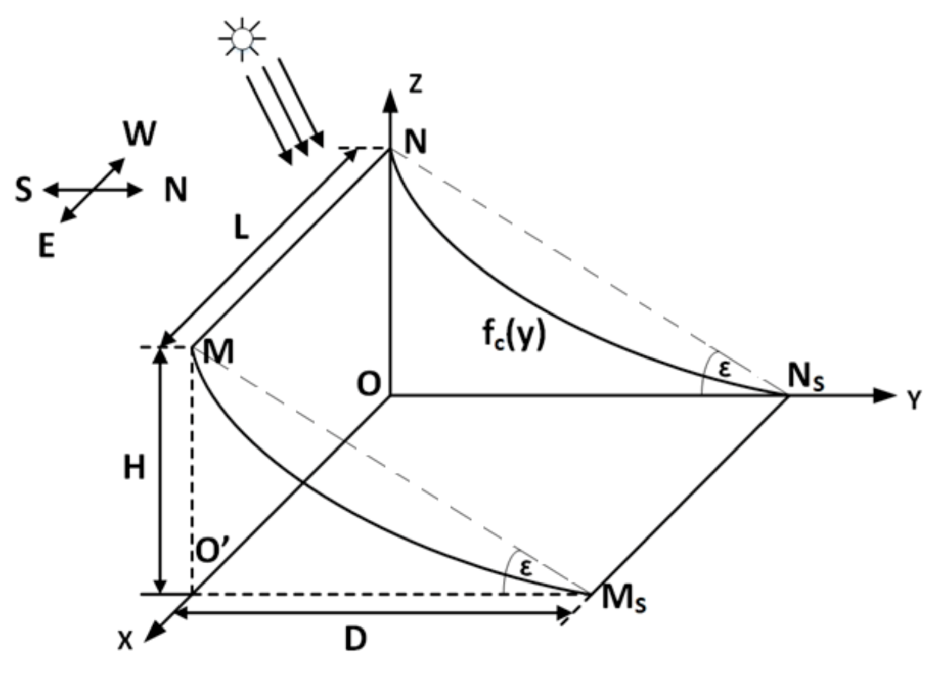
Figure 2.
Shadow components of line .
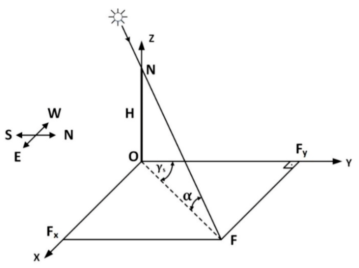
Figure 3.
Case (i).
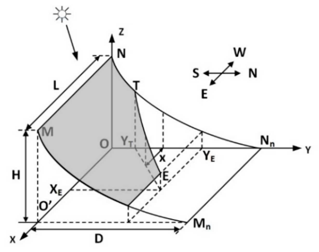
Figure 4.
Case (ii).
Figure 5.
Case (iii).
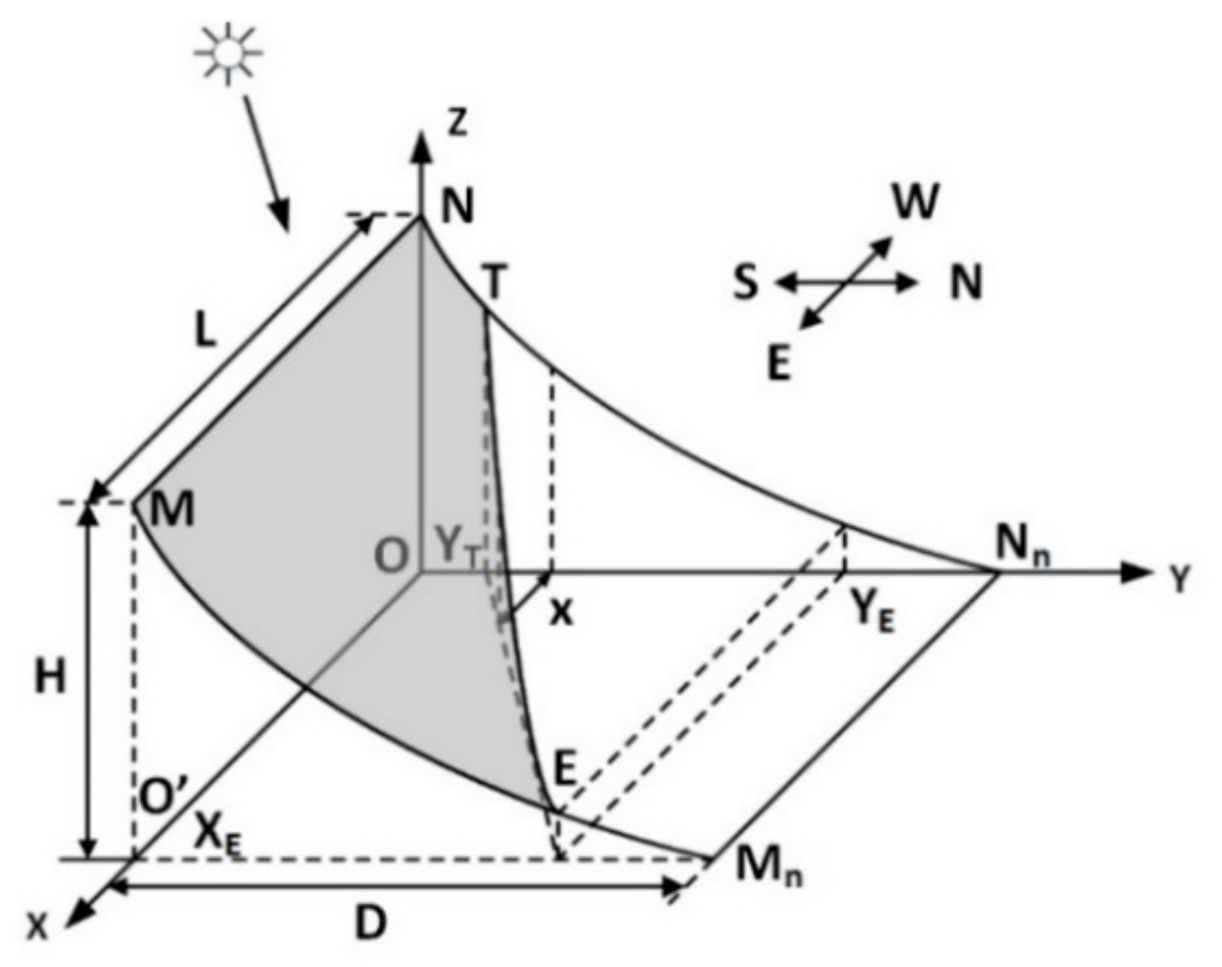
Figure 6.
State of shading: north-facing surface, latitude , .
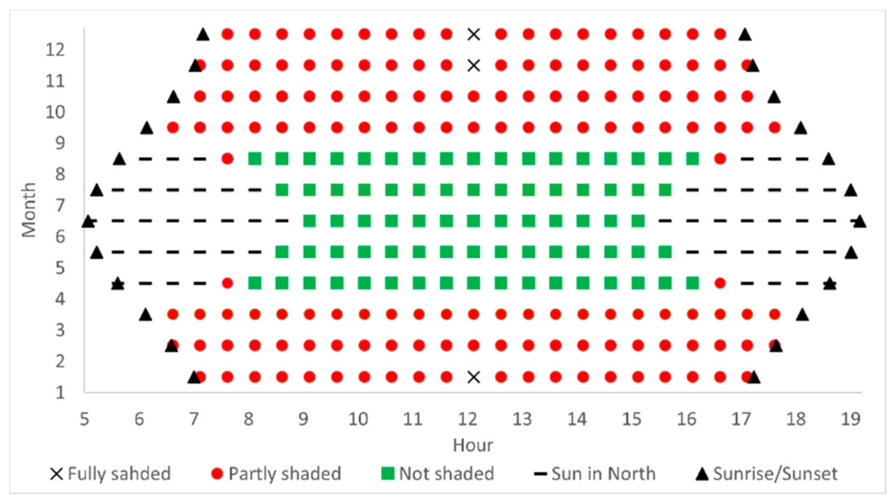
Figure 7.
State of shading: north-facing surface, latitude , .
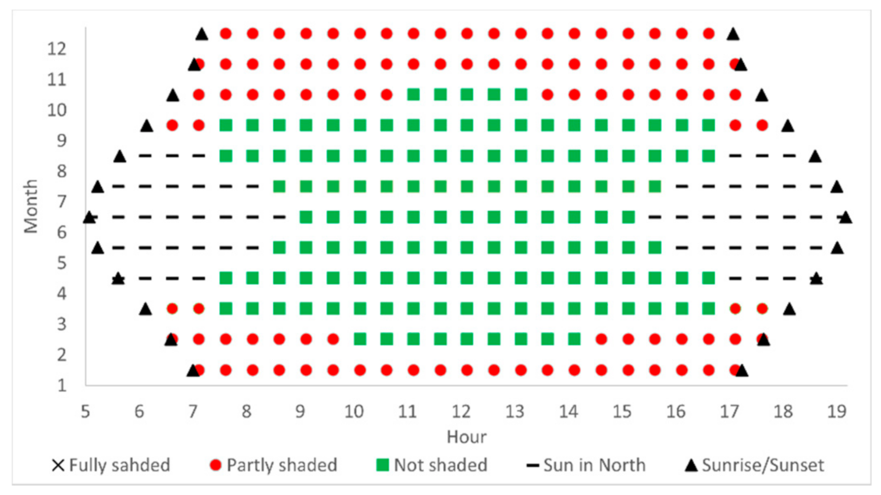
Figure 8.
State of shading: north-facing surface, latitude , .
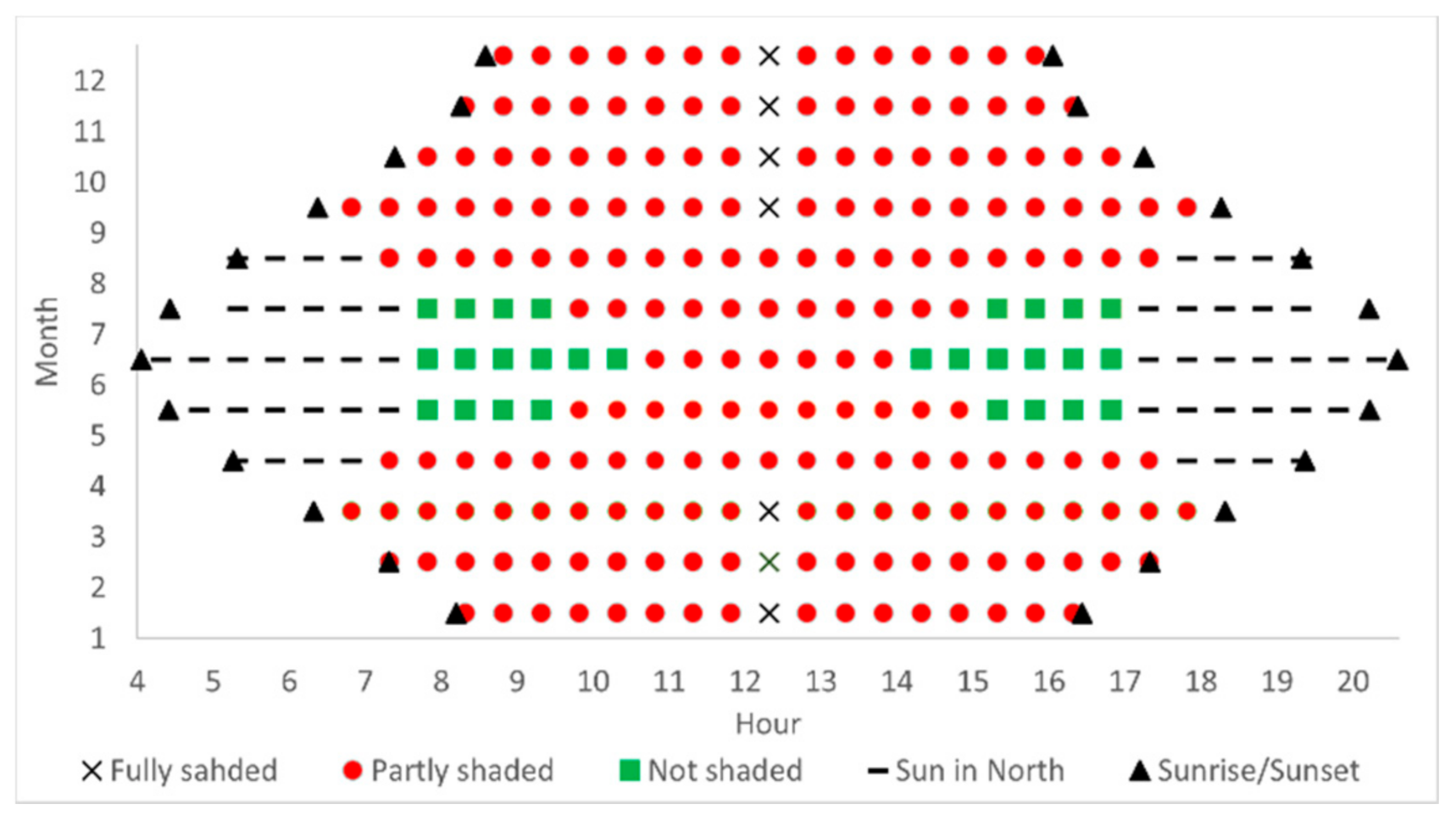
Figure 9.
State of shading: north-facing surface, latitude ,.
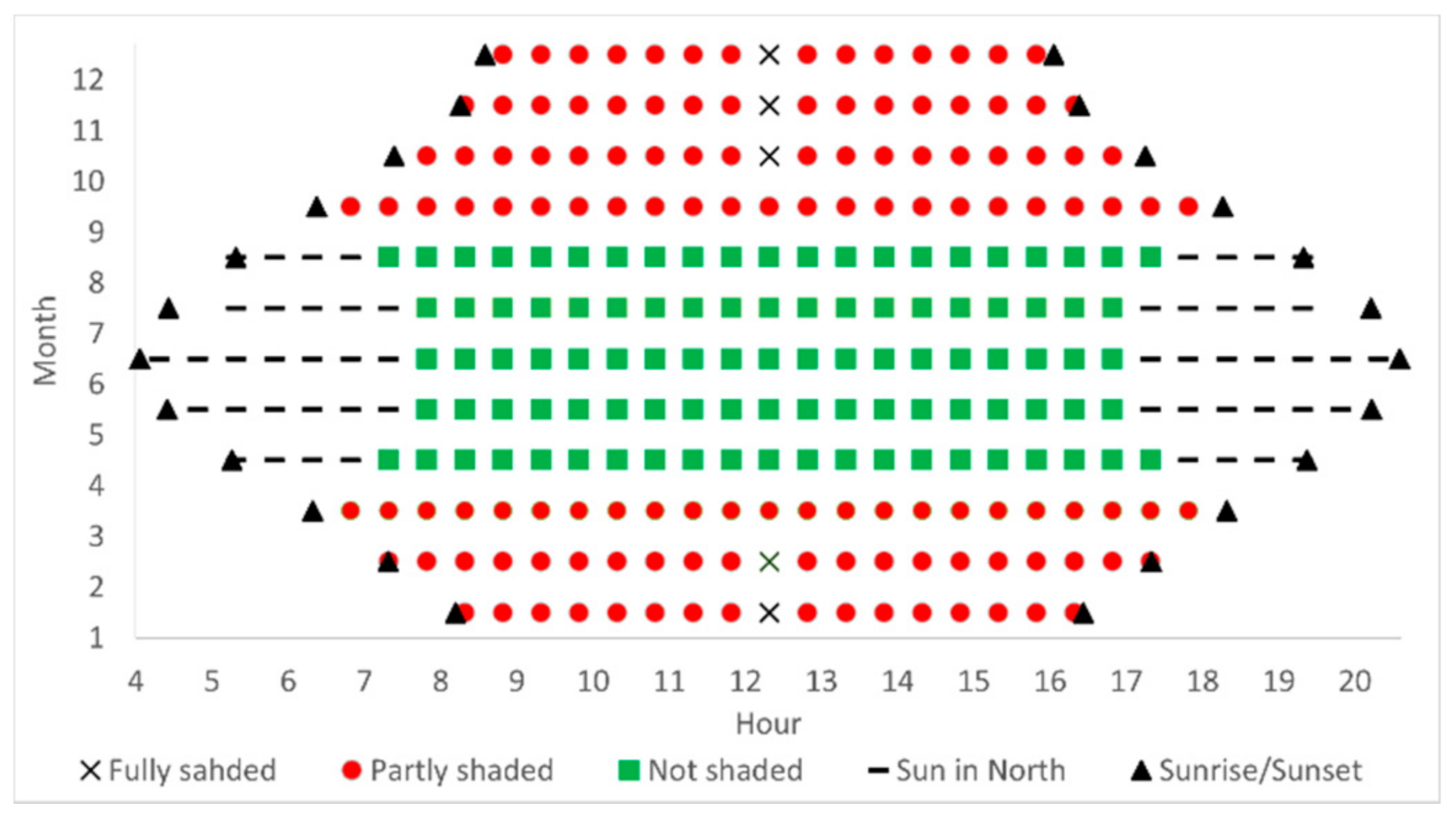
Figure 10.
State of shading: south-facing surface, latitude , .
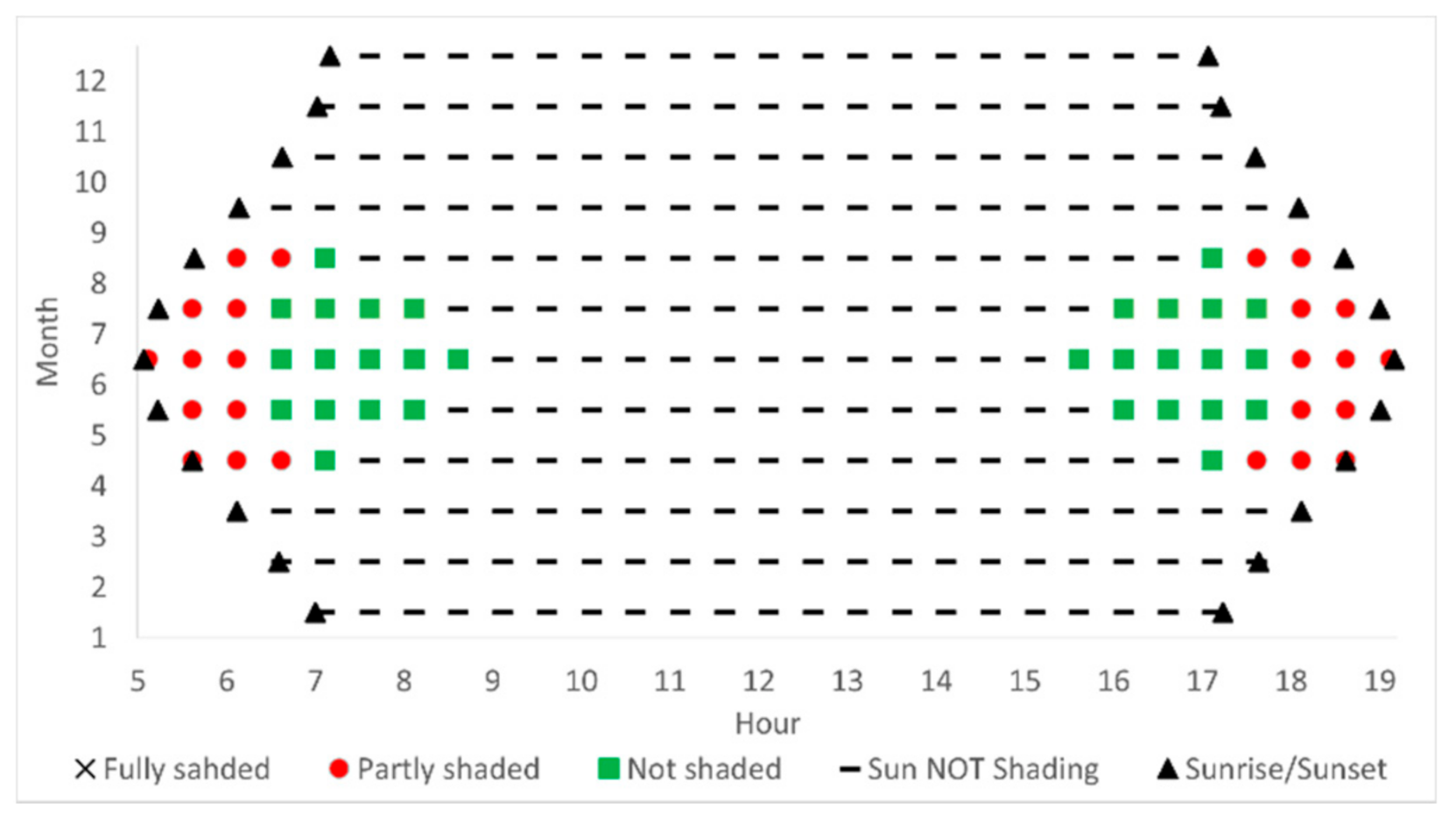
Figure 11.
State of shading: south-facing surface, latitude .
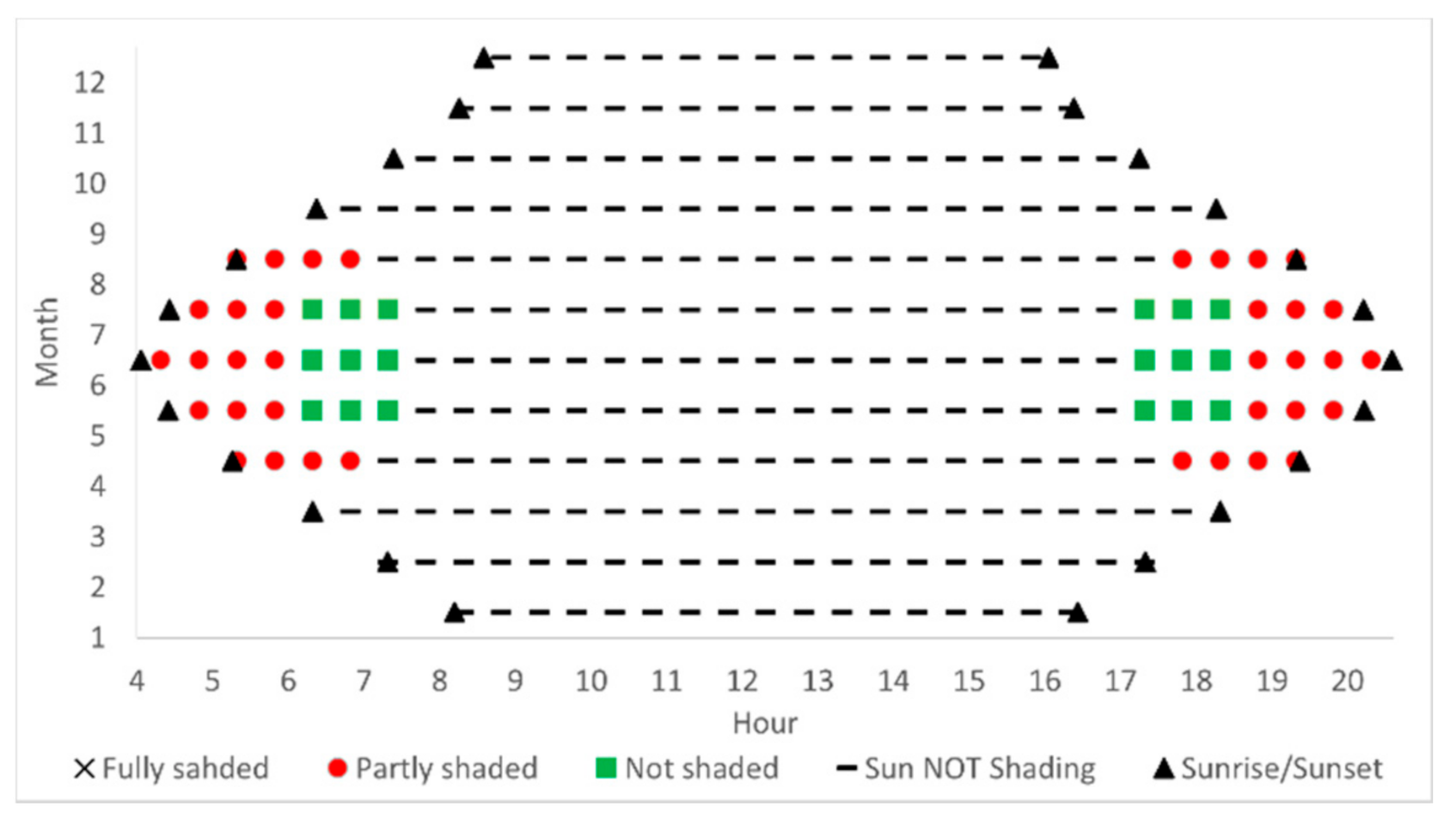
Figure 12.
State of shading: east-facing surface, latitude ,.
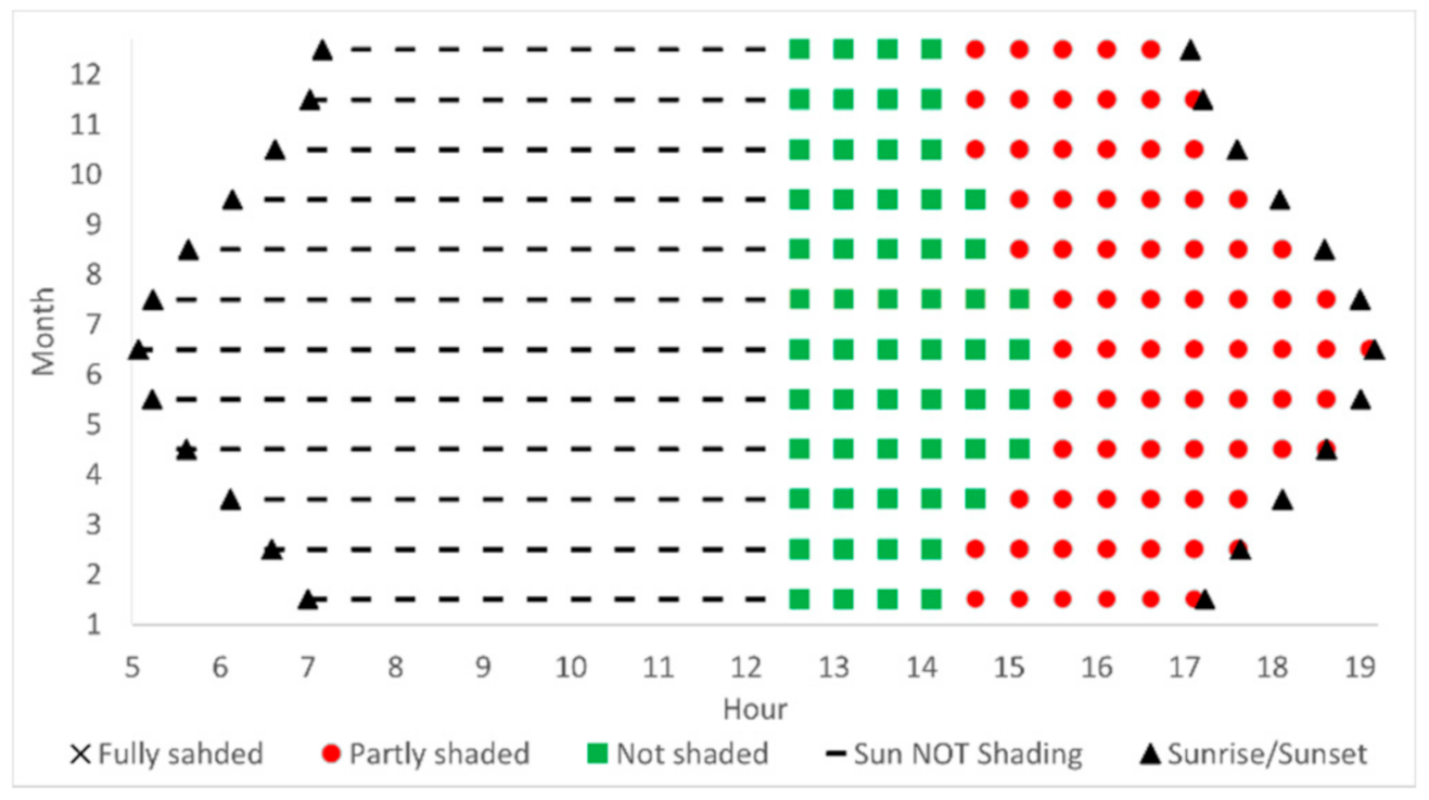
Figure 13.
State of shading: east-facing surface, latitude ,.


Table 1.
North-facing surface: yearly incident irradiation, .
| Sun in North Beam | No Shading Beam | Case (i) Beam | Case (ii) Beam | Case(iii) Beam | Diffuse | Global | |
|---|---|---|---|---|---|---|---|
| 94,476 | 628,571 | 277,196 | 4852 | 30,036 | 473,366 | 1,508,496 | |
| 36,527 | 202,945 | 187,349 | 8262 | 18,901 | 475,861 | 929,846 |
Table 2.
South-facing surface: yearly incident irradiation, .
| Sun in North Beam | No Shading Beam | Case (i) Beam | Case (ii) Beam | Case(iii) Beam | Diffuse | Global | |
|---|---|---|---|---|---|---|---|
| 1,216,521 | 66,093 | 0 | 0 | 26,779 | 473,366 | 1,782,758 | |
| 565,671 | 23,430 | 0 | 0 | 39,579 | 475,861 | 1,104,540 |
Table 3.
East-facing surface: yearly incident irradiation, .
| Sun in North Beam | No Shading Beam | Case (i) Beam | Case (ii) Beam | Case (iii) Beam | Diffuse | Global | |
|---|---|---|---|---|---|---|---|
| 789,655 | 240,273 | 105,712 | 2703 | 0 | 473,366 | 1,611,709 | |
| 408,874 | 72,101 | 103,179 | 5542 | 4941 | 475,861 | 1,070,497 |
Publisher’s Note: MDPI stays neutral with regard to jurisdictional claims in published maps and institutional affiliations. |
© 2021 by the authors. Licensee MDPI, Basel, Switzerland. This article is an open access article distributed under the terms and conditions of the Creative Commons Attribution (CC BY) license (https://creativecommons.org/licenses/by/4.0/).
Share and Cite
MDPI and ACS Style
Aronescu, A.; Appelbaum, J. Solar Radiation on a Parabolic Concave Surface. Energies 2021, 14, 2245. https://doi.org/10.3390/en14082245
AMA Style
Aronescu A, Appelbaum J. Solar Radiation on a Parabolic Concave Surface. Energies. 2021; 14(8):2245. https://doi.org/10.3390/en14082245
Chicago/Turabian StyleAronescu, Avi, and Joseph Appelbaum. 2021. "Solar Radiation on a Parabolic Concave Surface" Energies 14, no. 8: 2245. https://doi.org/10.3390/en14082245
Note that from the first issue of 2016, this journal uses article numbers instead of page numbers. See further details here.