Linear Regression Analysis and Techno-Economic Viability of an Air Source Heat Pump Water Heater in a Residence at a University Campus

Abstract

This study quantifies the potential of a 4.0 kW air source heat pump (ASHP) unit retrofitted to a 12.0 kW, 1000 L electric boiler coupled to a 1000 L storage tank. A data acquisition system was built to monitor the performance of the electric boiler and the ASHP water heater. The annual electrical energy saving and the load factor reduction from the electric boiler because of the ASHP unit retrofit was 34,805.94 kWh and 0.124. The net present value payback period of the ASHP system was 1.60 years. A Wilcoxon rank sum test was employed to compare both the volumes of hot water and electrical energy consumed by the two systems. Linear regression models of the daily volumes of hot water and electrical energy consumed by both systems were established. The results should be of great value to the management of universities that are considering energy-efficient interventions with a significant return on investment.

1. Introduction

Air source heat pump (ASHP) systems are widely used in the domain of sanitary water heating for their ability to act as both renewable and energy-efficient technologies. The energy and cost savings from installing ASHP water heaters as replacements for electric boilers can be determined through analytical methods using experimental data. Therefore, it is very important to conduct research into solution to the technological, environmental and socio-economic challenges through integrated demand management and energy efficiency intervention in student residences on a university campus. The majority of student residences provide sanitary hot water from electric boilers. These are inefficient devices, having a storage capacity greater than 500 L and heating achieved by a resistance element [1]. The energy factor of an electric boiler is less than 1. The input electrical energy consumed by the heating element is always greater than the output thermal energy stored by the water in the storage tank because of standing losses [2]. Significant energy savings could be obtained if electric boilers were replaced by ASHP water heaters. An ASHP water heater can turn one unit of input electrical energy into two to four units of useful output thermal energy during the vapour compression refrigeration process [3,4,5]. The special characteristic of the heat pump water heater, which is associated with exemplary performance, is called the coefficient of performance (COP) [6]. An ASHP water heater may reduce the power consumed during hot water heating by more than 50% when retrofitted to an existing electric boiler [6]. The COP of an ASHP water heater is influenced by the design of the components that make up the heat pump unit’s closed-loop circuit, the thermophysical properties of the refrigerant, the heating loads and the ambient conditions [7]. The threshold temperature of sanitary hot water can be set at 55 °C to prevent the growth of the bacteria (Legionella) and ensure optimal operation of the ASHP water heater [8]. In South Africa, the distribution of electrical energy consumed in the residential sector is such that 43, 12.3, 10.2, 9.9, 8.6 and 11.2% are allocated to the water heater, washing machine, electric stove, electric heater, fridge and small appliances, respectively [9]. Using coal as base load for electricity generation in thermal coal power plants is linked to greenhouse gas emissions [10]. The global warming potential associated with greenhouse gases (primarily carbon dioxide) stands at 510 million tons, of which 45% originates from the generation of electricity from coal [11]. The COP of an ASHP water heater depends strongly on the ambient temperature with respect to other weather parameters (relative humidity, wind speed) [12]. Mathioulakis et al. [13] employed an artificial neural network to predict the energy performance indices and the quantities characterizing an ASHP water heater operating at a high level of accuracy between measured and model outputs. The authors demonstrated that the correlation coefficients were greater than 0.999. The input parameters were the ambient air temperature in the evaporator and the water temperature at the inlet of the condenser of the ASPH unit. Tangwe et al. [14] developed robust multiple linear regression models to predict both the power consumed and the COP of an ASHP water heater. The input parameters were the outlet and the inlet water temperatures of the ASHP unit, the volume of water heated, the ambient temperature and the relative humidity. The determination coefficients between the measured and model outputs were greater than 0.987. Park et al. [15] developed both numerical methods and mathematical models of a hybrid heat pump water heater and a gas-fired heater to characterize the system performance. The authors also used their methods and models to estimate the economic benefits of the hybrid heat pump system. Pritchard et al. [16] used both the fundamental models of this system and a regression model to determine the space conditioning savings and cost of water heating in a restaurant compared to conventional gas and electric water heaters. Korolija et al. [17] used regression models to predict different HVAC system energy requirements. They confirmed the high accuracy of their predictions through statistical analysis over a pre-calculated data set comprised of 23,049 possible scenarios. The electrical energy saving from retrofitting an electric boiler with an ASHP unit depends on the volume of hot water consumption. In the winter months (May, June, July and August), hot water demand is usually higher than in the summer months (January, February, March, April, September, October, November and December) even though the COP is usually lower [18]. It is important to note that, unlike a solar water heater, an ASHP water heater can operate throughout the year giving an annual COP greater than 2 in any region of South Africa [19]. Commercial ASHP water heaters performed better than residential ASHP water heaters because of the type of compressor, condenser and expansion valves used. The up-front and installation costs of an ASHP heater is higher relative to that of an electric boiler [20], but despite the higher capital cost, the payback period is economically favourable [21]. Rankin et al. (2004) conducted a techno-economic analysis of a commercial ASHP water heater by implementing an in-line methodology during installation to optimize the design. The approach resulted in a reduction in life-cycle cost by a factor of 2.4 [22]. Lloyd and Kerr (2008) performed an energy payback analysis for an electric-boost solar flat plate heat pump system as a function of both COP and hot water usage for a given value of embodied energy. The findings revealed that a high water usage rate is required for a good energy payback time [23]. Keinath and Garimella (2017) conducted an experiment to compare the economic benefits of a gas-fired heat pump over a non-condensing gas unit and showed that the payback period of the gas-fired heat pump was four years shorter and the energy factor was above 1.5 [24]. Wang et al. [25] conducted an energy, exergy, economic and environmental analysis of an air source transcritical CO₂ heat pump water heater and determined that the payback period was less than 1 year and the CO₂ reduction was 378.01 tons. Experimental research conducted in South Africa demonstrated that both the split and integrated types of residential ASHP water heaters are viable technologies for sanitary hot water heating [26]. Eskom’s rollout of residential ASHP water heaters to replace inefficient geysers was an integrated demand-management intervention. The rebate/rollout scheme was intended to reduce both the demand and consumption of energy. Eskom’s residential ASHP water heaters rebate scheme served as part of the solution to reduce the demand on the national grid [27]; however, he rebate program was discontinued at the end of 2015 due to a lack of funding to sustain the scheme [28].

The study sought to demonstrate the quantitative and statistical benefits of using a 4 kW ASHP unit to retrofit a 12 kW electric boiler (consisting of a 1000 L tank and an additional 1000 L storage tank) in a postgraduate female residence with 70 students at the University of Fort Hare in South Africa. Additionally, the study took a conservative approach by applying robust linear regression models to correlate the daily volumes of hot water consumed using electrical energy from the boiler and from the ASHP water heater. Experiments on hot water heating by the electric boiler were conducted from January to December 2016, while experiments on heating by the ASHP water heater were conducted from January to December 2017. It is crucial to note that part of the preliminary results from the study had been published in the Industrial and Commercial Use of Energy conference proceeding in 2019 [29].

2. Objectives

To execute the study, the following primary objectives were established.

i.

To determine the reduction in the annual power, load factor and energy consumption after retrofitting an existing electric boiler with an ASHP unit.

ii.

To establish linear correlations of the daily volumes of hot water consumed to the electrical energy consumed by the electric boiler and the ASHP water heater in summer and winter.

iii.

To compare the daily volumes of hot water and electrical energy consumed by the electric boiler and the ASHP water heater, for both summer and winter using the Wilcoxon rank sum test.

iv.

To determine the annual cost saving and the payback period of the ASHP system.

v.

To conduct an ANOVA multiple comparison test to verify if any significant difference existed among the groups for average month-day volume of hot water and the electrical energy consumed by the heating devices during summer and winter.

3. Theory and Calculations

The electrical energy consumed by the electric boiler or the ASHP water heater is the product of the electrical power consumed and the time used during the heating period and is given by Equation (1).

$$\mathrm{E}=\mathrm{P}\mathrm{t}$$

(1)

where, $\mathrm{E}$ is the electrical energy consumed, $\mathrm{P}$ is the electrical power consumed and $\mathrm{t}$ is the time taken.

The thermal energy gained by the stored water in the storage tanks of the ASHP water heater is the product of the mass of water heated, the specific heat capacity of the water and the temperature difference between the water at the outlet and the inlet of the ASHP unit during the heating cycle and is given by Equation (2).

$$\mathrm{Q} =\mathrm{m}\mathrm{c} ({\mathrm{T}}_2-{\mathrm{T}}_1)$$

(2)

where, $\mathrm{Q}$ is the thermal energy gained, $\mathrm{m}$ is the mass of the water heated, $\mathrm{c}$ is the specific heat capacity of water, ${\mathrm{T}}_2$ is the temperature of water at the outlet of the ASHP unit and ${\mathrm{T}}_1$ is the temperature of water at the inlet of the ASHP unit.

The COP of the ASHP water heater is the ratio of the useful output thermal energy gained by the stored water to the input electrical energy consumed during the vapour compression refrigeration cycle and is given by Equation (3).

$$\mathrm{C}\mathrm{O}\mathrm{P}=\frac{\mathrm{Q}}{\mathrm{E}}$$

(3)

where, $\mathrm{COP}$ is the coefficient of performance, $\mathrm{Q}$ is the thermal energy gained and $\mathrm{E}$ is the electrical energy consumed.

The load factor of the electric boiler or the ASHP water heater is the ratio of the energy consumed over a 24 h period to the product of the maximum power and the period (24 h) and is given by Equation (4).

$$\mathrm{LF}=\frac{\mathrm{E} \mathrm{over} 24 \mathrm{h}}{{\mathrm{P}}_{\max }\times 24 \mathrm{h}}$$

(4)

where, $\mathrm{LF}$ is the load factor, $\mathrm{E}$ is the electrical energy consumed and ${\mathrm{P}}_{\max }$ is the maximum power consumed.

The electrical energy saving is calculated using a conservative approach: the difference between the electrical energy consumed by the electric boiler and the electrical energy consumed by the ASHP water heater on identical months. This assumption was reasonable as the volume of the average daily hot water consumed by the students from the both systems exhibited a negligible variation, a difference of 0.01%.

The simple payback period of a technology is the ratio of the capital cost and the product of the annual energy saving and tariff rate [30]. The simple payback period (SPB), may be expressed as shown in Equation (5).

$$\mathrm{S}\mathrm{P}\mathrm{B}=\frac{\mathrm{C}\mathrm{a}\mathrm{p}\mathrm{i}\mathrm{t}\mathrm{a}\mathrm{l} \mathrm{cost}}{\mathrm{A}\mathrm{n}\mathrm{n}\mathrm{u}\mathrm{a}\mathrm{l} \mathrm{e}\mathrm{n}\mathrm{e}\mathrm{r}\mathrm{g}\mathrm{y} \mathrm{s}\mathrm{a}\mathrm{v}\mathrm{i}\mathrm{n}\mathrm{g}\times \mathrm{t}\mathrm{a}\mathrm{r}\mathrm{r}\mathrm{i}\mathrm{f}}$$

(5)

The capital cost of a technology, takes into consideration both the upfront (principal) cost and the maintenance costs. The maintenance costs of an ASHP water heater include replacing the water filter and capacitor and their disposal at the end of their lifespan (approximately 15 years) [31].

The net present value (NPV) of money incorporates the concept that the value of money today is higher than it will be in the future. The NPV is influenced by factors such as inflation and interest rates and both affect money adversely over time [31]. The net present value (NPV) of money given an annual hike in tariff rate (r%) and future value (FV) for a number of years (n) is given in Equation (6).

$$\mathrm{N}\mathrm{P}\mathrm{V}=\frac{\mathrm{F}\mathrm{V}}{{\left(1+\mathrm{r}\right)}^{\mathrm{n}}}$$

(6)

It may be accepted without doubt that a technology is deemed to be economically viable if the payback period is significantly less than its stipulated lifespan as prescribed by the manufacturer.

The uncertainties derived from calculations as a result of the error measurements from a set of independent variables according to Meyer [32] is given in Equation (7).

$${\mathrm{w}}_{\mathrm{r}}=\left[{\left[{\mathrm{w}}_1\frac{\partial \mathrm{R}}{\partial {\mathrm{X}}_1}\right]}^2+{\left[{\mathrm{w}}_2\frac{\partial \mathrm{R}}{\partial {\mathrm{X}}_2}\right]}^2+\dots \dots \dots \dots +{\left[{\mathrm{w}}_{\mathrm{n}}\frac{\partial \mathrm{R}}{\partial {\mathrm{X}}_{\mathrm{n}}}\right]}^2\right]$$

(7)

where: $\mathrm{R}$ is the given function; $w_r$ is the total uncertainty; ${\mathrm{X}}_1,{\mathrm{X}}_2\dots \dots .{\mathrm{X}}_{\mathrm{n}}$ are the independent variables and ${\mathrm{W}}_1,{\mathrm{W}}_2\dots \dots .{\mathrm{W}}_{\mathrm{n}}$ are the uncertainties in the independent variables.

The combined uncertainties obtained from the calculation as a result of both type A and type B uncertainties is given in Equation (8).

$$\mathrm{U}=\sqrt{{\mathrm{U}}_{\mathrm{A}}^2+{\mathrm{U}}_{\mathrm{B}}^2}$$

(8)

where ${\mathrm{U}}_{\mathrm{A}}=\frac{\mathsf{\sigma }}{\sqrt{\mathrm{n}}}$: ${\mathrm{U}}_{\mathrm{A}}$ = Type A uncertainty for a given metering or determine parameter; $n=$ number of experimental trials or data; $\sigma$ = standard deviation.

${\mathrm{U}}_{\mathrm{B}}=\frac{\mathrm{u}}{\sqrt{3}}$: ${\mathrm{U}}_{\mathrm{B}}=$ Type B uncertainty and is a function of the accuracy of the metering sensors or transducers and $u=$ accuracy of the metering sensors or transducers.

4. Uncertainty Analysis of the Measurements

The temperature sensor used was a 12 bit S-TMB temperature sensor having a measurement range from −40 to 100 °C (accuracy was ± 0.2 °C). The ambient temperature and relative humidity sensor used was a 12 bit S-THB temperature and relative humidity sensor with a temperature range from 0 to 50 °C (accuracy ± 0.21 °C), while the accuracy of the relative humidity was ±0.25% over a range from 0 to 99%. The flow meter used was a T-Minol 130 having a measurement range from 1 to 100 L/min, with an accuracy between 97 and 99%. The power and energy meter used was the TVER-E50B2, a class 2 power meter with an error uncertainty of 0.5%.

5. Error Analysis

The type A uncertainties were based on the means and the standard deviations from the recorded measurements and are shown in

Table 1. Uncertainties of the measured and derived quantities.

Quantity	Type A Uncertainty	Type B Uncertainty	Combined Uncertainty
Ambient temperature (°C)	±0.200	±0.120	±0.233
Relative humidity (%)	±0.250	±0.140	±0.286
Water flow rates into inlet of the ASHP unit (L/min)	±0.010	±0.006	±0.012
Power consumed by the ASHP system (kW)	±0.130	±0.003	±0.130
Inlet water temperature of the ASHP (°C)	±0.250	±0.120	±0.277
Outlet water temperature of the ASHP (°C)	±0.230	±0.120	±0.259
Average month-day electrical energy consumed (kWh)	±0.130	±0.025	±0.132
Average month-day thermal energy gained (kWh)	±0.190	±0.042	±0.195
Average month-day COPs	±0.260	±0.203	±0.330

. The type B uncertainties are determined with reference to the accuracy of the sensors or the derived uncertainty by employing Equation (7). The total number of measurements or derived values for each parameter (ambient temperature, relative humidity, water flow rates into inlet of split type, ASHP unit, power consumed by the ASHP water heater, inlet and outlet water temperature of the split type ASHP, electrical energy consumption by month-day time of use, thermal energy gained and time of use month-day COP) were 1090. The combined uncertainties of the ambient temperature, relative humidity, water flow rates into inlet of the split type ASHP unit, power consumed by the ASHP system, the water temperature into the inlet and outlet of the ASHP unit were ±0.233 °C, ±0.286%, ±0.012 L/min, ±0.120 kW, ±0.277 °C and ±0.259 °C, respectively, and were obtained using the combined uncertainty formula in Equation (8) [33]. Furthermore, the combined uncertainties of the electrical energy consumed, the thermal energy gained and the COP of the ASHP water heater was ±0.132 kWh, ±0.195 kWh and ±0.330.

6. Statistical Tests

Statistical tests were conducted to compare two volumetric groups (daily volumes of hot water consumption from the electric boiler and the ASHP water heater in summer, and hot water consumption from the electric boiler and the ASHP water heater in winter). In addition, statistical tests were conducted to compare two daily electrical energy consumption groups of the electric boiler and the ASHP water heater for summer and winter, respectively. The Wilcoxon rank sum tests were used to compare the two groups. Secondly, one-way ANOVA tests were used to compare the four energies consumed and the volumetric groups of the electric boiler and the ASHP water heater. Both tests were used because the statistical analysis involved the testing of significant differences between the two groups, and this was conducted with the Wilcoxon rank sum test. It also involved the comparison among more than two groups (four) and was executed with one-way ANOVA tests in conjunction with the multiple comparison tests.

6.1. Wilcoxon Rank Sum Test

The Wilcoxon rank sum test is a nonparametric test for two populations or groups when the samples are independent. If x and y are independent samples with different sample sizes, the test statistic that the rank sum returns is the rank sum of the first sample [34,35]. The Wilcoxon rank sum test is equivalent to the Mann–Whitney U-test, which is a nonparametric test for equality of population medians of two independent samples X and Y.

In the Mann–Whitney $\mathrm{U}$-test, $\mathrm{U}$ is the number of times a $\mathrm{y}$ precedes an $\mathrm{x}$ in an ordered arrangement of the elements in the two independent samples $\mathrm{X}$ and $\mathrm{Y}$. It is related to the Wilcoxon rank sum statistic in the following way: If $\mathrm{X}$ is a sample of size $\mathrm{nX}$, then the relationship is given according to Equation (9).

$$\mathrm{U}=\mathrm{W}-\frac{\mathrm{n}\mathrm{X}\left(\mathrm{n}\mathrm{X}+1\right)}{2}$$

(9)

6.2. Wilcoxon Algorithms

For a two-sided test of medians with unequal sample sizes, the test statistic that the rank sum returns is the rank sum of the first sample. It should be noted that, p = rank sum (x, y) returns the p-value of a two-sided Wilcoxon rank sum test. Furthermore, the rank sum test tests the null hypothesis that data in x and y are samples from continuous distributions with equal medians against the alternative that they are not. The test assumes that the two samples are independent although x and y may have different lengths. In addition, (p, h) = rank sum (x, y) further returns a logical value indicating the test decision. The result h = 1, indicates a rejection of the null hypothesis and h = 0, indicates a failure to reject the null hypothesis at the 5% significance level.

6.3. One-Way ANOVA

One-way ANOVA is a trivial linear model. The one-way ANOVA model is given in Equation (10).

$${\mathrm{y}}_{\mathrm{ij}}={\mathsf{\alpha }}_{\mathrm{j}}+{\mathsf{\epsilon }}_{\mathrm{ij}}$$

(10)

The main assumptions of the model are

i.

${\mathrm{y}}_{\mathrm{ij}}$ is an observation in which i represent the observation number and j represents a different group of the predictor variable y.

ii.

All ${\mathrm{y}}_{\mathrm{ij}}$ are independent.

iii.

${\mathrm{a}}_{\mathrm{j}}$ represents the population mean for the jth group.

iv.

${\mathsf{\epsilon }}_{\mathrm{ij}}$ is the random error, independent and normally distributed, with zero mean and constant variance, (${\mathsf{\epsilon }}_{\mathrm{ij}}~\mathrm{N}\left(0,{\mathsf{\sigma }}^2\right)$).

v.

The model assumes that the columns of $\mathrm{y}$ are the constant ${\mathsf{\alpha }}_{\mathrm{j}}$ plus the error component ${\mathsf{\epsilon }}_{\mathrm{ij}}$.

ANOVA tests the hypothesis that all group means are equal versus the alternative hypothesis that at least one group is different from the others and is given in Equation (11).

$${\mathrm{H}}_0:{\mathsf{\alpha }}_1={\mathsf{\alpha }}_2=\dots ={\mathsf{\alpha }}_{\mathrm{k}} \mathrm{and} {\mathrm{H}}_1:\mathrm{not} \mathrm{all} \mathrm{group} \mathrm{means} \mathrm{are} \mathrm{equal}$$

(11)

The one–way ANOVA of the among groups in y, abbreviated as anova1(y), tests the equality of column means for the data in matrix y, where each column is a different group and has the same number of observations. Alternatively, anova1(y, group) tests the equality of group means, specified in the group, for the data in vector or matrix y.

6.4. ANOVA Table

The ANOVA table captures the variability of the model by source, the F-statistic for testing the significance of this variability and the p-value for deciding on the significance of this variability [36]. The p-value is correct only if the distribution is independent, normally distributed and has a constant variance [37]. The standard ANOVA table has the form given in

Table 2. Standard form of an ANOVA table.

Source	Sum Square SS	Degree of Freedom df	Mean Square MS	F-Statistic	p-Value (Prob > F)
Group (between)	SSR	k − 1	MSR = SSR/k − 1	MSR/MSE	P(Fk − 1,N − k) > F
Error (within)	SSE	N − k	MSE = SSE/N − k
Total	SST	N − 1

. The terms SSR, SSE and SST represented the sum squares of the between groups, sum squares of the within groups and the sum squares of the total groups respectively. The term k stands for the number of between groups (number of columns, if the groups are expressed as a matrix) while N represents the number of within groups.

7. Materials and Methods

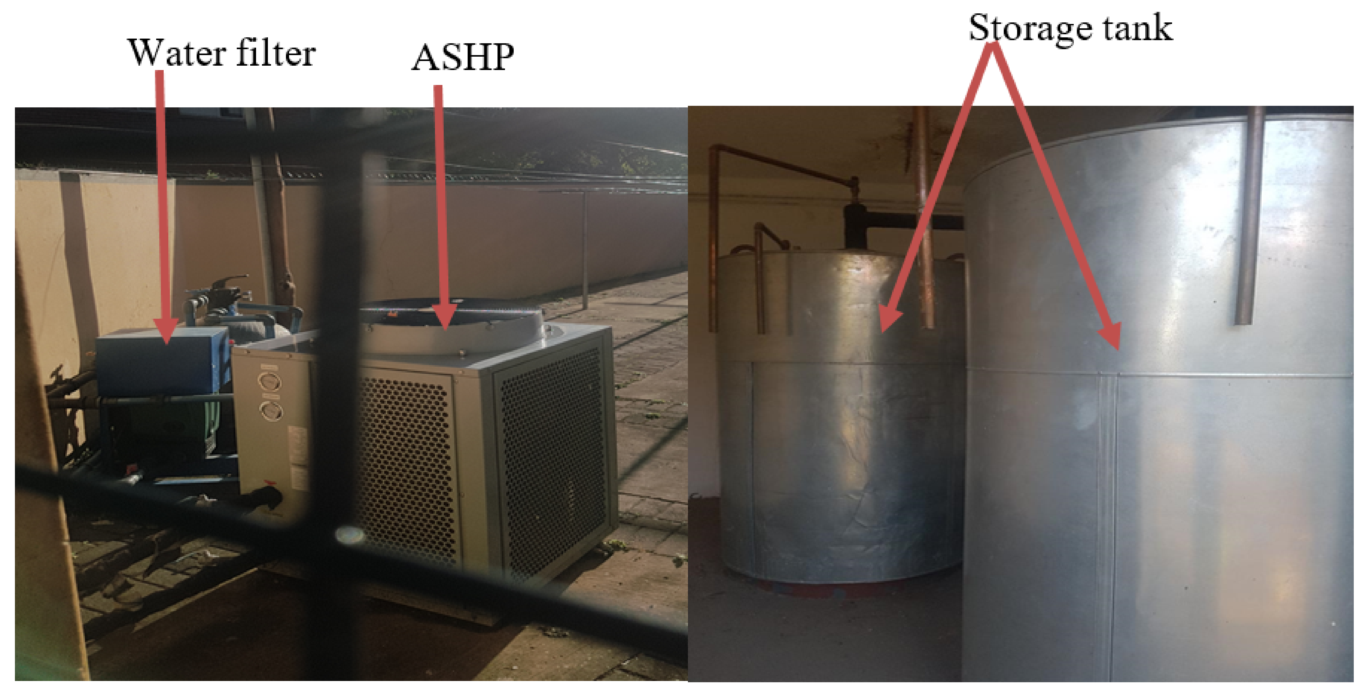
7.1. Materials

The list of hot water devices, sensors and transducers used in the study is shown in

Table 3. Hot water devices, sensors and transducers used in the experiment.

Materials	Quantity
Power meter	1
Flow meter	2
Temperature sensors	5
Ambient temperature and relative humidity sensor	1
12 kW, 1000 L electric boiler with an additional 1000 L storage tank	1
4.0 kW input ASHP unit	1
Water filter	1
Data logger	1
Waterproof enclosure	1

.

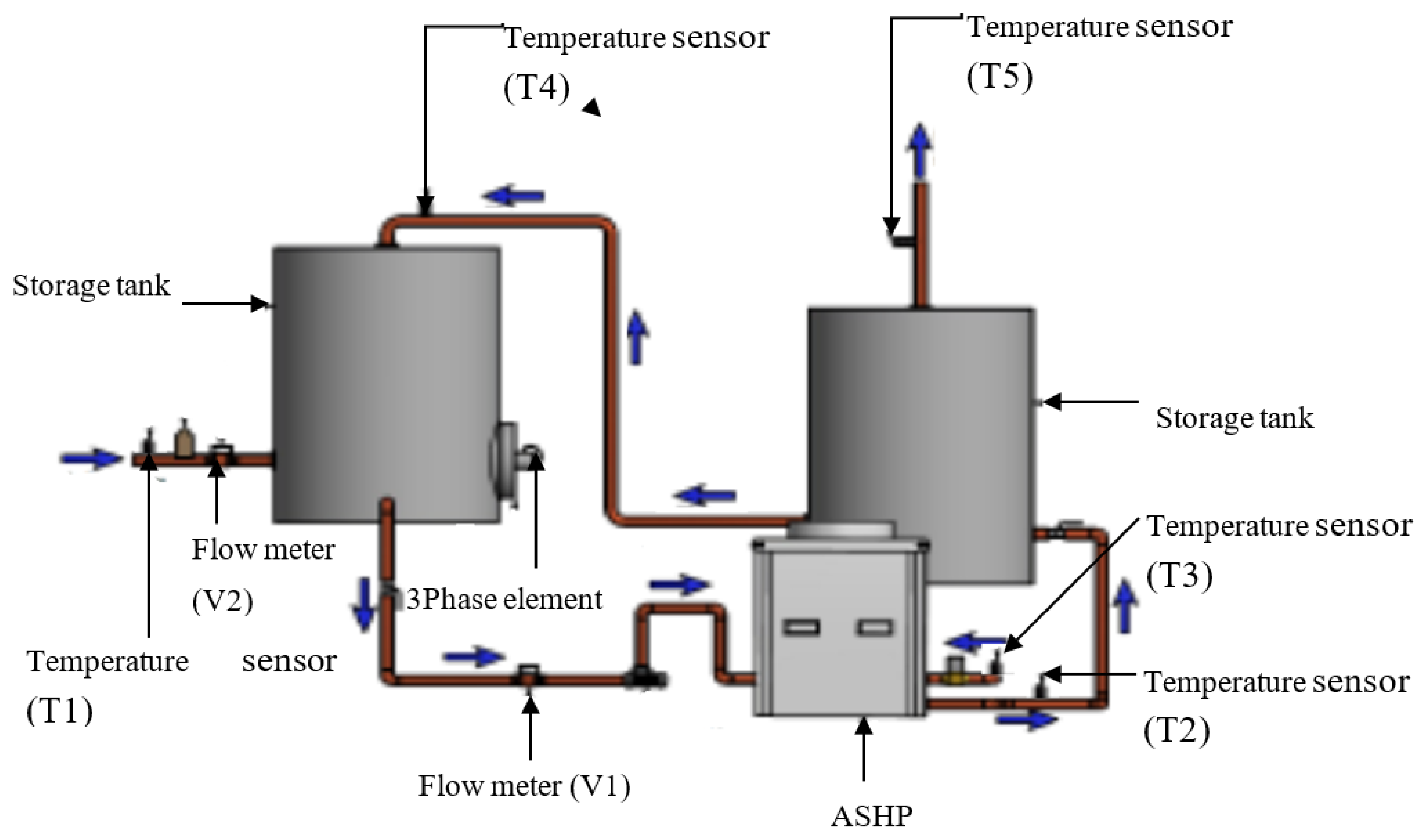
7.2. Experimental Setup

The electric boiler (comprised of 12 kW heating element and two storage tanks of 1000 L each), filter and ASHP unit are shown in Figure 1. The 12 kW heating element is contained in the electric boiler with a 1000 L tank capacity, while the other 1000 L served as a backup storage tank. The schematic diagram of the ASHP unit retrofitted to the electric boiler is shown in Figure 2. Sensors were installed at various locations in the hot water heating system: a temperature sensor (T1) was installed by drilling at the inlet of the cold water pipe of the electric boiler, which feeds the makeup water into the storage tanks containing the heating element. This sensor measured the temperature of the makeup water. Two temperature sensors (T4 and T5) were installed by drilling at the outlet pipes of the two hot water storage tanks and measured the temperature of the hot water supplied to the residence. A temperature sensor (T3) was installed by drilling at the inlet of the ASHP unit on the copper pipe that fed the inlet of the ASHP unit with water from the storage tank. A temperature sensor (T2) was installed by drilling in the copper pipe at the outlet of the ASHP unit, allowing the heated water to exit from the outlet of the ASHP unit to the storage tank. All the installed water temperature sensors were well-sealed to prevent water from leaking through the drilled holes at the designated locations on the copper pipes. A flow meter (V1) was installed on the pipe that led to the inlet of the ASHP unit and measured the volume of hot water heated by it, during vapour compression refrigeration cycles. A second flow meter (V2) was installed on the inlet pipe that supplied makeup water into the storage tank and measured the volume of hot water consumed by the students in the residence. A power meter was installed on the electrical supply line, powering either the 12 kW resistive element of the electric boiler or the ASHP unit. The power meter measured the power consumed by the electric boiler or the ASHP unit. An ambient temperature and relative humidity sensor were installed in the vicinity of the hot water devices and measured the ambient temperature and the relative humidity. All the sensors and transducers were connected to a data logger and configured to log at 5 min intervals throughout the monitoring period: when hot water production was achieved by the electric boiler (before the implementation phase) and by the ASHP system (after the implementation phase). All sensors and transducers were properly insulated to avoid interference from external sources.

The methodology of the study is divided into two parts:

i.

The electrical energy and the volume of hot water consumed using the electric boiler and the ASHP water heater during the monitoring period.

ii.

The derivation of mathematical models for the two hot water devices and the conduction of a techno-economic analysis of the ASHP water heater.

8. Results and Discussion

8.1. Modelling the Daily Electrical Energy Consumed

The processed data of the daily volumes of hot water and electrical energy consumed by the electric boiler and the ASHP water heater were partitioned into 70 and 30% of the trained data set and test data set, respectively. Linear regression models to correlate the volumes of daily hot water consumption to the daily electrical energy consumption by the electric boiler and the ASHP water heater were determined for both summer and winter. Figure 3 shows a sample of the daily volumes of hot water and electrical energy consumed from the two heating systems.

Table 4. Forcing and scaling constants of the mathematical models in summer and winter seasons.

Input Parameter	Constants	Constant Symbols	Scaling Constant	Output Parameter	Mathematic Model
Volumes of water consumed from boiler in summer (Vbs)	Forcing Scaling	A B	−44 0.098	Electrical energy consumed by boiler in summer (Ebs)	Ebs = A + B (Vbs) Ebs = −51 + 0.10 (Vbs)
Volumes of water consumed from ASHP in summer (Vas)	Forcing Scaling	A B	0.49 0.02	Electrical energy consumed by ASHP in summer (Eas)	Eas = A + B (Vas) Eas = 0.27 + 0.02 (Vas)
Volumes of water consumed from boiler in winter (Vbw)	Forcing Scaling	A B	−331.63 0.243	Electrical energy consumed by boiler in winter (Ebw)	Ebw = A + B (Vbw) Ebw = −331 + 0.243 (Vbw)
Volumes of water consumed from ASHP in winter (Vaw)	Forcing Scaling	A B	188.75 0.120	Electrical energy consumed by ASHP in winter (Eaw)	Eaw = A + B (Vaw) Eaw = −188 + 0.12 (Vaw)

A = Forcing constant, B = Scaling constant, Vbs = Volume of hot water consumed from boiler in summer, Vbw = Volume of hot water consumed from boiler in winter, Vas = Volume of hot water consumed from ASHP in summer, Vaw = Volume of hot water consumed from ASHP in winter, Ebs = Electrical energy consumed by boiler in summer, Ebw = Electrical energy consumed by ASHP in winter, Eas = Electrical energy consumed by ASHP in summer, Eaw = Electrical energy consumed by ASHP in winter.

shows the forcing and scaling constants of the mathematical models of the daily electrical energy consumed with the volumes of hot water consumed as a predictor for the two hot water heating systems for both seasons.

8.1.1. Modelling the Daily Electrical Energy Consumed during the Summer Period

The daily volumes of hot water consumed and the equivalent electrical energy consumed by both the electric boiler and the ASHP water heater based on the trained data set are represented in Figure 3. It showed that electrical energy consumption increased as the volume of hot water consumption increased. The linear regression models correlated the volumes of the hot water consumed with the electrical energy consumed by both the electric boiler and the ASHP water heater. The plots show positive gradients (red and blue lines) with that of the electric boiler as 0.10 kWh/L and for the ASHP water heater as 0.02 kWh/L. The axis intercepts for the electrical energy consumed for the electric boiler and the ASHP water heater were −51 and 0.27 kWh, respectively. These negative and the very small positive energy consumption figures suggested that input factors other than the volume of hot water consumed contributed to the electrical energy consumption but were not included in the derived models. The determination coefficients (r-square) of the modelled and measured electrical energy consumed by the electric boiler and the ASHP water heater were 0.96 and 0.97, respectively. In addition, the root mean square error (RMSE) of the measured and modelled daily electrical energy consumed by the electric boiler and ASHP water heater was 1.33 and 0.23, respectively. The very good determination coefficients and the root mean square errors suggested that the modelled equations of the electric boiler and the ASHP water heater were highly accurate with respect to the measured data set. The modelled electrical energy that were consumed mimicked the measured values. Hence, by using the daily volumes of hot water consumed as the input parameter, the mathematical models can be accepted as predictors of the daily electrical energy consumed by the electric boiler and the ASHP water heater.

The forcing and scaling constants of the linear regression models that correlate the daily volumes of hot water usage with the electrical energy usage is shown in Table 4. A forcing constant is a lump arbitrary constant that takes into consideration other input parameters not included in the model equation. The forcing constant helps the models accurately predict the expected or measured outputs. The forcing constants (A) of the electric boiler and the ASHP water heater were −51 and 0.27 kWh, respectively. The scaling constants (B) were 0.10 and 0.02 kWh/L, for the electric boiler and the ASHP water heater, respectively.

The test data set was used to validate the linear regression models for the electric boiler and the ASHP water heater. The validated data set was coherently and accurately predicted by the developed linear regression models of the electric boiler and the ASHP water heater with a sufficient confidence level. The consumption of the validated daily electrical energy and the predicted daily electrical energy demonstrated no significant difference. The p-value for the validated data set and the predicted values for the electric boiler was 0.942, while the p-value for the ASHP water heater was 0.954.

8.1.2. Modelling the Daily Electrical Energy Consumed during the Winter Period

The daily volumes of hot water consumed and the corresponding electrical energy consumed by the electric boiler and the ASHP water heater using the trained data set is shown in Figure 3. It was observed that daily electrical energy consumption increased in a direct proportion to the volumes of hot water consumed for the two hot water heating devices. These plots showed positive slopes (green and black lines) of 0.243 and 0.120 kWh/L, for the electric boiler and the ASHP water heater, respectively. The intercepts at the axis of the electrical energy consumed for the electric boiler and the ASHP water heater were −331.63 and 188.75 kWh, respectively. These negative and positive energy consumption figures imply there are other predictors different from the volume of hot water consumed that influenced electrical energy consumption but were not taken into account in the building and developing of the mathematical models. The determination coefficients (r-square) of the modelled and the measured electrical energy consumed by the electric boiler and the ASHP water heater, were 0.97 and 0.98, respectively. The determined root mean square errors from the measured and modelled electrical energy consumed by the electric boiler and the ASHP water heater were 0.21 and 0.08, respectively. These exceptional values of the determination coefficients and the root mean square errors of the electric boiler and the ASHP water heater confirmed that the modelled outputs demonstrated negligible discrepancies with the measured values.

The forcing and scaling constants of the linear regression models of the daily electrical energy consumed in relation to the volumes of the hot water consumed is provided in Table 4. The forcing constants (A) of the electric boiler and the ASHP water heater were −331.63 and 188.75 kWh, while the scaling constants (B) were 0.243 and 0.120 kWh/L, respectively.

The test data set was used to validate the derived linear models of the electric boiler and the ASHP water heater. The validated daily electrical energy consumption mimicked the modelled daily electrical energy consumption with reasonable confidence. The p-values for the electric boiler and the ASHP water heater were 0.965 and 0.972, respectively.

8.2. Comparison of the Electrical Energy and Volumes Consumed by Both Systems

The daily consumption of the volumes of hot water and the electrical energy consumed by the electric boiler and the ASHP water heater were compared, using the Wilcoxon rank sum test for both summer and winter.

8.2.1. Comparison of the Daily Volumes and Energy Consumed Using Wilcoxon Rank Sum Test during the Summer Season

The Wilcoxon rank sum test of the daily volumes of hot water consumed from the electric boiler and the ASHP water heater showed a p-value of 0.4704 with the logical value of the test decision (h) as 0 at a 5% significance level. The large p-value confirmed that no significant difference existed between the two groups of the daily volumes of hot water consumed during the summer. However, h = 0 revealed the logical decision that there was a failure to reject the null hypothesis test at a 5% significance level. On the contrary, the comparison of the daily electrical energy consumed by the electric boiler and the ASHP water heater during this time showed that a significant difference existed between the two groups with a p-value of 3.05 × 10⁻⁹. The logical value of the test decision (h) was 1, thus rejecting the null hypothesis that both groups originated from a continuous distribution with equal medians.

8.2.2. Comparison of the Volumes and Energy Consumed Using Wilcoxon Rank Sum Test during the Winter

The Wilcoxon rank sum test of the daily volumes of hot water consumed from the electric boiler and the ASHP water heater depicted a p-value of 0.070, and the logical value of the test decision (h) was 0 at a 5% significance level. This implied that the p-value was slightly greater than 0.05 and there existed no significant difference between the two groups of the daily volumes of hot water consumed. The logical value of the test decision (h) was 0 and revealed a failure to reject the null hypothesis test at a 5% significance level. Furthermore, the comparison of the daily electrical energy consumed by the electric boiler and the ASHP water heater during the winter affirmed that a significant difference existed between the two groups as the p-value was 7.45 × 10⁻⁶. The logical value (h) of the test decision was 1, indicating a rejection of the null hypothesis of the groups emanating from a continuous distribution with equal medians.

8.3. Average Month-Day Performance of the Electric Boiler and ASHP Water Heater

The average month-day performance of the electric boiler and the ASHP water heater is presented in

Table 5. Average month-day performance of the hot water heating devices.

Month	Device	E/kWh	V/L	LF	Pmax/kW	P/kW	t/h	COP
January	Boiler	126.70	1740.00	0.45	12.48	12.05	10.50
	ASHP	36.26	1700.00	0.37	4.70	4.40	8.24	3.40
February	Boiler	125.40	1730.00	0.45	12.46	12.22	10.26
	ASHP	34.63	1705.00	0.36	4.67	4.33	8.00	3.52
March	Boiler	127.10	1750.00	0.46	12.47	12.11	10.50
	ASHP	35.73	1720.00	0.37	4.67	4.41	8.10	3.46
April	Boiler	137.85	1900.00	0.46	12.45	12.11	11.38
	ASHP	39.47	1885.00	0.37	4.67	4.34	9.10	3.00
May	Boiler	140.10	1940.00	0.46	12.37	12.05	11.63
	ASHP	42.30	1920.00	0.38	4.67	4.42	9.57	2.85
June	Boiler	134.82	1964.00	0.47	12.39	12.19	12.12
	ASHP	40.26	1961.00	0.35	4.67	4.19	10.18	2.88
July	Boiler	138.63	1955.00	0.47	12.38	12.06	11.50
	ASHP	41.79	1930.00	0.37	4.67	4.41	9.50	2.97
August	Boiler	137.85	1953.00	0.46	12.38	12.10	11.75
	ASHP	41.45	1937.00	0.37	4.67	4.34	9.75	2.90
September	Boiler	138.20	1830.00	0.46	12.46	12.30	11.24
	ASHP	35.80	1810.00	0.37	4.67	4.42	8.10	3.12
October	Boiler	138.70	1835.00	0.48	12.39	12.19	11.44
	ASHP	35.40	1830.00	0.36	4.67	4.40	8.05	3.14
November	Boiler	122.58	1710.00	0.47	12.38	12.22	10.03
	ASHP	33.24	1700.00	0.37	4.67	4.43	7.50	3.48
December	Boiler	122.40	1725.00	0.46	12.38	12.23	10.00
	ASHP	33.86	1720.00	0.37	4.67	4.44	7.63	3.39
Annual-	Boiler	132.53	1836.00	0.46	12.41	12.15	11.03
average	ASHP	37.52	1818.20	0.37	4.67	4.38	08.64	3.10

E = Electrical energy consumed, V = Volume of water consumed, Pmax = Maximum power, P = Average power, LF = Load factor, t = Time, COP = Coefficient of performance.

. The parameters that were used for each of the months over the monitoring period to compare the operating performance of the electric boiler and the ASHP water heater were

• the electrical energy consumed,
• the volume of hot water consumed,
• the load factor,
• the maximum and average power, and
• the COP.

The average month-day electrical energy consumed by the electric boiler was significantly greater than that of the ASHP water heater as depicted in Table 5. The average month-day volume of hot water consumed by the electric boiler and the ASHP water heater was 1836 and 1818.2 L, respectively. The average month-day load factor of the electric boiler and the ASHP water heater was 0.463 and 0.368, respectively. The average electrical power consumed by the electric boiler was almost three times that of the ASHP water heater. The average month-day duration during which the electric boiler was in operation was approximately 2.5 h more with reference to the operating time of the ASHP water heater. The average month-day COP of the ASHP water heater was between 2.85 and 3.52 and the annual average COP was 3.10. Therefore, the annual average electrical power consumed, the electrical energy consumed and the load factor were lower with the ASHP water heater in operation compared to the electric boiler.

8.4. Monthly Electrical Energy Saving

The monthly electrical energy consumed by the electric boiler and the ASHP water heater, as well as the derived energy saving, is shown in

Table 6. Monthly performance of hot water devices.

Month	Boiler’s Electrical Energy/kWh	ASHP Electrical Energy/kWh	COP of ASHP	Saving /kWh
January	3927.7	1124.06	3.4	2803.64
February	3511.2	969.64	3.52	2541.56
March	3940.1	1107.63	3.46	2832.47
April	4135.5	1184.1	3	2951.4
May	4343.1	1311.3	2.85	3031.8
June	4044.6	1207.8	2.88	2836.8
July	4297.53	1295.49	2.97	3002.04
August	4273.35	1284.95	2.9	2988.4
September	4146	1074	3.12	3072
October	4299.7	1097.4	3.14	3202.3
November	3677.4	997.2	3.48	2680.2
December	3794.4	1049.66	3.39	2744.74
Annual total	48,390.58	13,703.23		34,687.35

. It shows that for each of the months, the electrical energy consumed by the electric boiler was over three times that of the ASHP water heater. This indicated that the ASHP water heater is an energy efficient device for sanitary hot water heating having an annual average COP of 3.10. The total electrical energy consumed by the electric boiler (from January to December 2016) and the ASHP water heater (from January to December 2017), was 48,390.58 kWh and 13,703.23 kWh, respectively. The average daily hot water consumed from the electric boiler and the ASHP water heater was 1865.25 L and 1847.88 L, respectively, during the monitoring period. The percentage difference in the average daily volume of hot water consumed was 0.01%, which is almost negligible. Hence, the annual energy saving from the retrofitting of the existing electric boiler with an ASHP unit, was 34,687.35 kWh. This demonstrated that the ASHP water heater can perform with an excellent COP throughout the year. A substantial monthly electrical energy saving was achieved by the implementation of an ASHP water heater as a replacement for the existing electric boiler.

8.5. Techno-Economic Cost Analysis of the Installed ASHP System

The techno-economic life cost analysis of the ASHP system envisages the viability of the technology on the basis of the payback period (PB) using the net present value of money (NPV). The NPV of money is of a higher value than the future value of money (FV). This may be the result of both inflation and interest rates on the capital cost. The incurred cost of the ASHP system included the capital cost of the ASHP unit, the water filter, the maintenance cost of replacing the water filter bag, the cost of installation and the disposal cost of the ASHP system. The capital cost of the ASHP unit, the water filter and the installation of the ASHP system was R 80,000.00. The cost of maintenance was R 1000.00, which was the cost incurred for the replacement of the water filter and was implemented every four years. The disposal cost was R 2000.00 and will be incurred at the end of the lifespan of the ASHP system. Hence, the total cost incurred for the entire lifespan (15 years) of the ASHP system, will be R 85,000.00 as shown in

Table 7. Techno-economic life cost analysis of the ASHP system.

Year	No of Year	Saving /kwh	TARRIF/6.5% Rise Per Year	FV /R	NPV /R	Cost Incurs /R	Cumulative Net Cost Saving/R
2016	0.00					80,000.00	00000.00
2017	1.00	34,805.94	1.575	54,819.36	51,473.57	0.00	54,819.36
2018	2.00	34,805.94	1.65375	57,560.32	50,748.59	0.00	105,568.0
2019	3.00	34,805.94	1.736438	60,438.34	50,033.82	0.00	155,601.8
2020	4.00	34,805.94	1.823259	63,460.26	49,329.12	1000.00	204,930.9
2021	5.00	34,805.94	1.914422	66,633.27	48,634.35	0.00	253,565.2
2022	6.00	34,805.94	2.010143	69,964.93	47,949.36	0.00	301,514.6
2023	7.00	34,805.94	2.110651	73,463.18	47,274.01	0.00	348,788.6
2024	8.00	34,805.94	2.216183	77,136.34	46,608.18	1000.00	395,396.8
2025	9.00	34,805.94	2.326992	80,993.16	45,951.73	0.00	441,348.5
2026	10.00	34,805.94	2.443342	85,042.81	45,304.52	0.00	486,653.0
2027	11.00	34,805.94	2.565509	89,294.95	44,666.43	0.00	531,319.5
2028	12.00	34,805.94	2.693784	93,759.7	44,037.32	1000.00	575,356.8
2029	13.00	34,805.94	2.828474	98,447.69	43,417.08	0.00	618,773.9
2030	14.00	34,805.94	2.969897	103,370.1	42,805.57	0.00	661,579.4
2031	15.00	34,805.94	3.118392	108,538.6	42,202.68	2000.00	703,782.1

R = South Africa rand, FV = Future value, PV = Present value.

. The Eskom’s initial tariff was R 1.50/kWh and the annual percentage of tariff hike used was 5%. The annual cost saving, in terms of the future value of money, is the product of the annual energy saving and the Eskom’s tariff with the rates of tariff hike included. The annual cost saving, as the net present value of money (NPV) is a combination of the annual cost saving of the future value of money (FV), with the annual rate of return (r), taken into consideration. The relation of the net present value of money (NPV) with respect to the future value of money (FV), the annual rate of return (r) and the number of years (n) is provided in Equation (6). The annual rate of return (r) used on the techno-economic cost analysis was 6.5%. The breakdown of the life cost economic analysis of the ASHP system is presented in Table 7. The annual energy saving by retrofitting the existing electric boiler with the ASHP system was 34,805.94 kWh. The future value and the net present value of the annual cost savings are also shown. The payback period of the ASHP system was determined to be 1.60 years, which means that the total net present value cost saving, after the reduction of the cost incurred at the end of the lifespan (2031) of the ASHP system, will be R 618,782.10.

8.6. One-Way ANOVA Test among the Derived Groups Means

The groups means were classified into two categories of average month-day electrical energy consumed and average month-day volume of hot water consumed with the hot water heating devices during the different heating seasons. The four group means of the average-month-day electrical energy consumed include

• The average month-day electrical energy consumed by the electric boiler during the summer (energy consumed by the boiler in summer),
• The average month-day electrical energy consumed by the ASHP water heater during the summer (energy consumed by the ASHP in summer),
• The average month-day electrical energy consumed by the electric boiler during the winter (energy consumed by the boiler in winter),
• The average month-day electrical energy consumed by the ASHP water heater during the winter (energy consumed by the ASHP in winter).

The four groups means of the average month-day volume of hot water consumed from the hot water heating devices were

• The average month-day volume of hot water consumed from the electric boiler during the summer (volume consumed from the boiler in summer),
• The average month-day volume of hot water consumed from the ASHP water heater during the summer (volume consumed from the ASHP in summer),
• The average month-day volume of hot water consumed from the electric boiler during the winter (volume consumed from the boiler in winter),
• The average month-day volume of hot water consumed from the ASHP water heater during the winter (volume consumed from the ASHP in winter).

The one-way ANOVA test was conducted on the derived group means of electrical energy and volume of hot water consumed. The summer months were January, February, March, April, September, October, November and December while the winter months were May, June, July and August during the performance monitoring periods.

8.6.1. One-Way ANOVA Test among the Derived Groups’ Means of Electrical Energy Consumed

Table 8. One-way ANOVA table of the average month-day electrical energy consumed.

Source	Sum Square SS	Degree of Freedom df	Mean Square MS	F-Statistic	p-Value (Prob > F)
Group (between)	56,295.8	3	18,765.3	805.66	5.12 × 10−21
Error (within)	465.8	20	23.3
Total	56,761.6	23

shows that the sum of the squares for the between-group means was 56,295.8 while that of the within-group means was 465.8. The total sum of squares for the group means was the sum of the between-group means and the within-group means and was 56,761.6. The degree of freedom for the between-group means and the within-group means was 3 and 20. The total degree of freedom was 23. The mean square between the group means was 18,765.3 while the mean square within the group means was 23.3. The F-statistic of the group mean of the average month-day electrical energy consumed was 805.66. The large value of the F-statistic revealed that the ratio of the mean square of the between-group means and the within-group means for the distribution was very large and resulted in a very small p-value of 5.12 × 10⁻²¹. The very small p-value meant there was at least a significant difference at a 5% significance level among the four group means.

Figure 4 shows the ANOVA plots for the four group means of the average month-day electrical energy consumed. The means of electrical energy consumption by the boiler in winter, the boiler in summer, the ASHP in winter and the ASHP in summer were 143.85, 130.26, 44.31 and 35.63 kWh, respectively. The figure shows that the distribution from each of the group means was distributed normally. The electric boiler consumed the most electrical energy and occurred during winter while the lowest was consumed by the ASHP water heater during the summer.

8.6.2. Multiple Comparison Test among the Derived Group Means of Electrical Energy Consumed

The multiple comparison test is an advanced ANOVA test used to show if there exists any significant difference between the pairwise groups at a 5% significance level among the four group means (energy consumed by the boiler in summer, by the ASHP in summer, the boiler in winter and by the ASHP in winter).

Table 9. Multiple comparison of the average month-day electrical energy consumed.

Group	Group	Lower Confidence Interval	Estimate	Upper Confidence Interval
Energy consumed by boiler in summer	Energy consumed by ASHP in summer	87.87	94.63	101.38
Energy consumed by boiler in summer	Energy consumed by boiler in winter	−21.86	−13.59	−5.32
Energy consumed by boiler in summer	Energy consumed by ASHP in winter	77.68	85.95	94.22
Energy consumed by ASHP in summer	Energy consumed by boiler in winter	−116.49	−108.22	−99.95
Energy consumed by ASHP in summer	Energy consumed by ASHP in winter	−16.95	−8.68	−0.40
Energy consumed by boiler in winter	Energy consumed by ASHP in winter	89.99	99.54	109.09

shows the multiple comparison matrices among the four group means of the average month-day electrical energy consumed. The lower and upper confidence intervals of the pairwise groups of the energy consumed by ASHP in summer and winter were −16.95 and −0.40, respectively, while the mean of the confidence intervals was −8.68. The confidence interval did not contain 0, and there was a significant difference at the 5% significance level. Furthermore, based on a similar interpretation of the rest of the five pairwise energy consumption groups (boiler and ASHP in summer; boiler in summer and winter; boiler in summer and ASHP in winter; ASHP in summer and boiler in winter; boiler and ASHP in winter), it can be shown that all the corresponding confidence intervals did not include 0. Hence, all the six pairwise group means were significantly different at the 5% significance level.

Figure 5 shows a multiple-comparison interactive graph of four pairwise group means of average month-day electrical energy consumption, and not one of them overlaps. Therefore, significant differences existed in energy consumption in all the group pairs: boiler/summer and ASHP/summer; boiler/summer, and boiler/winter; boiler/summer and ASHP/winter; ASHP/summer and boiler/winter; ASHP/summer and ASHP/winter; and boiler/winter and ASHP/winter.

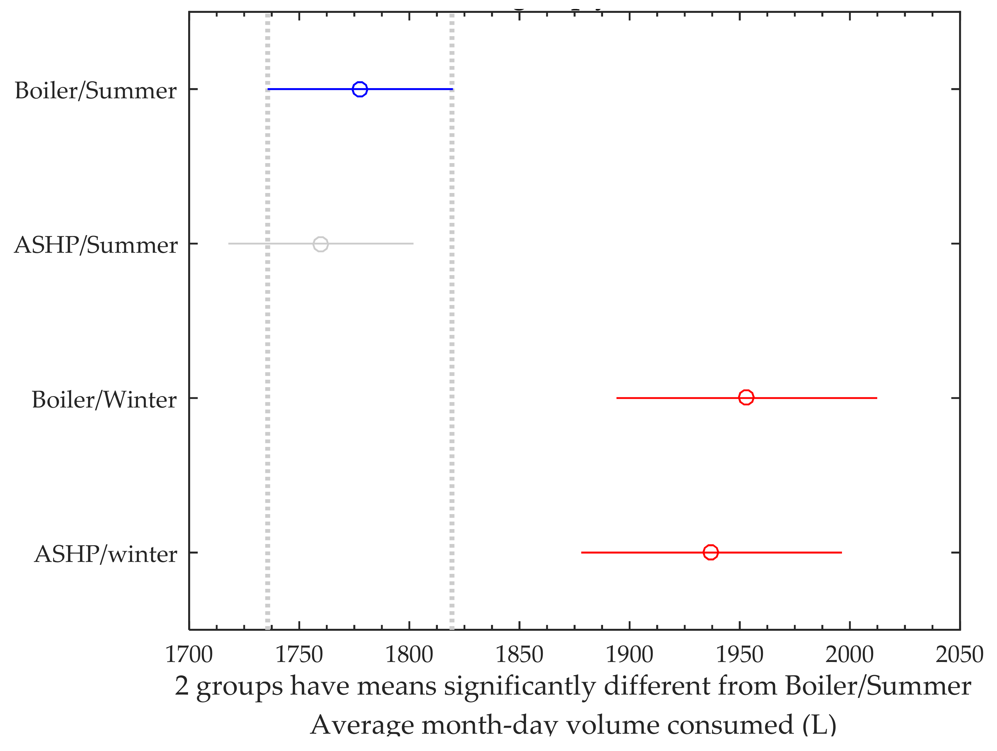
8.6.3. One-Way ANOVA Test among the Groups Means of Volume of Hot Water Consumed

Table 10. One-way ANOVA table of the average month-day volume of water consumed.

Source	Sum Square SS	Degree of Freedom df	Mean Square MS	F-Statistic	p-Value (Prob > F)
Group (between)	167,817.8	3	55,939.3	16.02	1.52 × 10−5
Error (within)	9845.9	20	3492.3
Total	237,663.7	23

, shows that the sum of the squares for the between-group means of the average month-day was 167,817.8, while that of the within-group means was 9845.9. The total sum of squares for the group means was 237,663.7. The degree of freedom for the between-group means and the within-group means were 3 and 20. The total degree of freedom was 23. The mean squared between the group means was 55,939.3 while the mean squared within the group means was 3492.3. The F-statistic of the group means of the average month-day volume of hot water consumed was 16.02. The large value of the F-statistic revealed that a very small p-value among the groups. The p-value was 1.52 × 10⁻⁵. The very small p-value, justified that, there is at least a significant difference at a 5% significance level.

Figure 6 shows the ANOVA plots for the four group means for average month-day volume of hot water consumed. The means of the volume consumed from the boiler in summer, the volume consumed from the ASHP in summer, the volume consumed from the boiler in winter and the volume consumed from the ASHP in winter was 1777.50, 1759.62, 1953.00 and 1937.00 L, respectively. The figure shows that the distribution of each of the group means was normally distributed as no outliers were detected. The largest volume of hot water was consumed from the electric boiler during the winter while the lowest volume was consumed from the ASHP water heater during the summer.

8.6.4. Multiple Comparison Test among the Group Means of Volume of Water Consumed

Table 11. Multiple comparison of the average month-day volume of hot water consumed.

Group	Group	Lower Confidence Interval	Estimate	Upper Confidence Interval
Volume consumed from boiler in summer	Volume consumed from ASHP in summer	−64.83	17.88	100.58
Volume consumed from boiler in summer	Volume consumed from boiler in winter	−276.79	−175.50	−74.21
Volume consumed from boiler in summer	Volume consumed from ASHP in winter	−260.79	−159.50	−58.21
Volume consumed from ASHP in summer	Volume consumed from boiler in winter	−294.66	−193.38	−92.09
Volume consumed from ASHP in summer	Volume consumed from ASHP in winter	−278.66	−177.38	−76.09
Volume consumed by boiler in winter	Volume consumed from ASHP in winter	−100.96	16.00	132.96

, shows a multiple comparison matrix among the four group means of average month-day volume of water consumed: (from the boiler in summer, from the ASHP in summer, from the boiler in winter and from the ASHP in winter). The two pairwise groups (volume consumed from the boiler and the ASHP in summer and from the boiler and the ASHP in winter) show the lower and upper confidence intervals as −64.83 and 100.58 and −100.96 and 132.96, respectively. Each of the confidence intervals contains 0, and the difference were not significant at 5% significance level. In accordance to the interpretation for the pairwise group comparison, the confidence intervals of the pairwise groups (volume consumed from the boiler in summer and in winter, the boiler in summer and the ASHP in winter, the ASHP in summer and the boiler in winter, the ASHP in winter and in summer), do not include 0 and were significantly different.

Figure 7 shows a multiple comparison interactive graph of the four group means of the average month-day volume of hot water consumed. The figure shows that two of the pairwise groups (volume consumed from the boiler and ASHP in summer and from the boiler and ASHP in winter) do overlap and therefore exhibited no significant difference. Figure 7 also showed that four of the pairwise groups (volume consumed from the boiler in summer and winter; the boiler in summer and ASHP in winter, the ASHP in summer and boiler in winter, the ASHP in summer and winter) among the four group means were disjoint. Therefore, there existed significant differences between each of the four pairwise groups.

9. Conclusions

Significant benefits were achieved by retrofitting an existing electric boiler with an ASHP unit in a student residence at a university campus to reduce demand and electrical energy consumption. The power consumed by the installed ASHP unit was almost three times lower than that of the existing electric boiler. The implementation of the ASHP unit as an energy efficient technology was accompanied by a reduction of the load factor. The Wilcoxon rank sum test was employed to show that a significant difference exists between the two groups of the daily electrical energy consumed by the ASHP water heater and the electric boiler for both the summer and winter. Nonetheless, the logical value of the decision test showed a rejection of the null hypothesis test for the two groups to be continuous and having equal medians. The annual average COP and the net present value payback period of the ASHP system was 3.10 and 1.60 years. The payback period may be further reduced provided the hot water consumed by the students in the residence increased and the tariff rates continued to increase. Finally, the operating performance of the ASHP water heater demonstrated that the ASHP system efficiently saved electrical energy in both the summer and winter. It is imperative that this technology be rolled out as a smart and energy efficient measure for the sanitary hot water heating of university residences. In addition to the very small p-value of 5.12 × 10⁻²¹ among the four group means of average month-day electrical energy consumed, the multiple comparison test was exploited to show that there exists a significant difference between all the six pairwise groups among the four group means.

References

1. Bott, C.; Dressel, I.; Bayer, P. State-of-technology review of water-based closed seasonal thermal energy storage systems. Renew. Sustain. Energy Rev. 2019, 113, 109241. [Google Scholar] [CrossRef]
2. Granade, H.C.; Creyts, J.; Derkach, A.; Farese, P.; Nyquist, S.; Ostrowski, K. Unlocking energy efficiency in the US economy. McKinsey Co. 2009, 1, 1–165. [Google Scholar]
3. Willem, H.; Lin, Y.; Lekov, A. Review of energy efficiency and system performance of residential heat pump water heaters. Energy Build. 2017, 143, 191–201. [Google Scholar] [CrossRef] [Green Version]
4. Tangwe, S.L. Demonstration of Residential Air Source Heat Pump Water Heaters Performance in South Africa: Systems Monitoring and Modelling. Ph.D. Thesis, University of Sunderland, Tyne and Wear, UK, 2018. [Google Scholar]
5. Staffell, I.; Brett, D.; Brandon, N.; Hawkes, A. A review of domestic heat pumps. Energy Environ. Sci. 2012, 5, 9291–9306. [Google Scholar] [CrossRef]
6. Morrison, G.L.; Anderson, T.; Behnia, M. Seasonal performance rating of heat pump water heaters. Sol. Energy 2004, 76, 147–152. [Google Scholar] [CrossRef]
7. Mohanraj, M.; Belyayev, Y.; Jayaraj, S.; Kaltayev, A. Research and developments on solar assisted compression heat pump systems–A comprehensive review (Part A: Modeling and modifications). Renew. Sustain. Energy Rev. 2018, 83, 90–123. [Google Scholar] [CrossRef]
8. Hollander, M.; Wolfe, D.A. Nonparametric Statistical Methods; John Wiley & Sons, Inc.: Hoboken, NJ, USA, 1999. [Google Scholar]
9. Proctor, C.R.; Dai, D.; Edwards, M.A.; Pruden, A. Interactive effects of temperature, organic carbon, and pipe material on microbiota composition and Legionella pneumophila in hot water plumbing systems. Microbiome 2017, 5, 130. [Google Scholar] [CrossRef] [PubMed]
10. Simcock, N.; Thomson, H.; Petrova, S.; Bouzarovski, S. (Eds.) Energy Poverty and Vulnerability: A Global Perspective; Routledge: London, UK, 2017. [Google Scholar]
11. Shin, H.C.; Park, J.W.; Kim, H.S.; Shin, E.S. Environmental and economic assessment of landfill gas electricity generation in Korea using LEAP model. Energy Policy 2005, 33, 1261–1270. [Google Scholar] [CrossRef]
12. Chua, K.J.; Chou, S.K.; Yang, W.M. Advances in heat pump systems: A review. Appl. Energy 2010, 87, 3611–3624. [Google Scholar] [CrossRef]
13. Mathioulakis, E.; Panaras, G.; Belessiotis, V. Artificial neural networks for the performance prediction of heat pump hot water heaters. Int. J. Sustain. Energy 2018, 37, 173–192. [Google Scholar] [CrossRef]
14. Tangwe, S.; Simon, M.; Meyer, E. Mathematical modeling and simulation application to visualize the performance of retrofit heat pump water heater under first hour heating rating. Renew. Energy 2014, 72, 203–211. [Google Scholar] [CrossRef]
15. Park, H.; Nam, K.H.; Jang, G.H.; Kim, M.S. Performance investigation of heat pump–gas fired water heater hybrid system and its economic feasibility study. Energy Build. 2014, 80, 480–489. [Google Scholar] [CrossRef]
16. Pritchard, B.A.; Beckman, W.A.; Mitchell, J.W. Heat pump water heaters for restaurant applications. Int. J. Ambient Energy 1991, 12, 59–68. [Google Scholar] [CrossRef]
17. Korolija, I.; Zhang, Y.; Marjanovic-Halburd, L.; Hanby, V.I. Regression models for predicting UK office building energy consumption from heating and cooling demands. Energy Build. 2013, 59, 214–227. [Google Scholar] [CrossRef]
18. Rezaie, B.; Dincer, I.; Esmailzadeh, E. Energy options for residential buildings assessment. Energy Convers. Manag. 2013, 65, 637–646. [Google Scholar] [CrossRef]
19. Available online: http://www.onsetcomp.com (accessed on 27 May 2013).
20. Hohne, P.A.; Kusakana, K.; Numbi, B.P. A review of water heating technologies: An application to the South African context. Energy Rep. 2019, 5, 1–19. [Google Scholar] [CrossRef]
21. Martinopoulos, G.; Papakostas, K.T.; Papadopoulos, A.M. Comparative analysis of various heating systems for residential buildings in Mediterranean climate. Energy Build. 2016, 124, 79–87. [Google Scholar] [CrossRef]
22. Rankin, R.; Rousseau, P.G.; van Eldik, M. Demand side management for commercial buildings using an inline heat pump water heating methodology. Energy Convers. Manag. 2004, 45, 1553–1563. [Google Scholar] [CrossRef]
23. Lloyd, C.R.; Kerr, A.S.D. Performance of commercially available solar and heat pump water heaters. Energy Policy 2008, 36, 3807–3813. [Google Scholar] [CrossRef]
24. Keinath, C.M.; Garimella, S. An energy and cost comparison of residential water heating technologies. Energy 2017, 128, 626–633. [Google Scholar] [CrossRef]
25. Wang, Y.; Ye, Z.; Song, Y.; Yin, X.; Cao, F. Energy, exergy, economic and environmental analysis of refrigerant charge in air source transcritical carbon dioxide heat pump water heater. Energy Convers. Manag. 2020, 223, 113209. [Google Scholar] [CrossRef]
26. Tangwe, S.L.; Simon, M. Quantification of the viability of residential air source heat pump water heaters as potential replacement for geysers in South Africa. J. Eng. Des. Technol. 2019, 17, 456–470. [Google Scholar] [CrossRef]
27. Kukard, W.C. The Adaptive Predictive Control of an Energy Efficient Central Water Heating System Applied in the South African Commercial Sector. Ph.D. Thesis, North-West University, Vanderbair Park, South Africa, 2016. [Google Scholar]
28. Tangwe, S.L.; Simon, M. Development of simplified benchmark models to predict the coefficient of performance of residential air source heat pump water heaters in South Africa. Energy Effic. 2019, 12, 1821–1835. [Google Scholar] [CrossRef]
29. De Swardt, C.A.; Meyer, J.P. A performance comparison between an air-source and a ground-source reversible heat pump. Int. J. Energy Res. 2001, 25, 899–910. [Google Scholar] [CrossRef]
30. Storesletten, K. Fiscal implications of immigration—A net present value calculation. Scand. J. Econ. 2003, 105, 487–506. [Google Scholar] [CrossRef] [Green Version]
31. Tangwe, S.; Manyi-Loh, C. An Economic-Cost Analysis of Commercial Air Source Heat Pump Water Heater in the University Campus. In Proceedings of the AIUE 17th Industrial and Commercial Use of Energy (ICUE) Conference 2019, Cape Town, South Africa, 26 November 2019; ISBN 978-0-6399647-4-4. Available online: https://ssrn.com/abstract=3650487 (accessed on 20 July 2020). [CrossRef]
32. Meyer, S.L. Data Analysis for Scientists and Engineers; Wiley: Hoboken, NJ, USA, 1975. [Google Scholar]
33. Tangwe, S.; Kusakana, K. A statistical methodology to compare the performance of residential air source heat pump water heaters. Int. J. Sustain. Energy 2020, 1–20. [Google Scholar] [CrossRef]
34. Gibbons, J.D.; Chakraborti, S. Nonparametric Statistical Inference, 5th ed.; Chapman & Hall/CRC Press; Taylor & Francis Group: Boca Raton, FL, USA, 2011. [Google Scholar]
35. Tangwe, S.; Simon, M.; Meyer, E. March. Quantifying Residential Hot Water Production Savings by Retrofitting Geysers with Air Source Heat Pumps. In Proceedings of the 2015 International Conference on the Domestic Use of Energy (DUE), Cape Town, South Africa, 31 March–1 April 2015; IEEE: Piscataway, NJ, USA, 2015; pp. 235–241. [Google Scholar]
36. Kachelmeier, S.J.; Messier, W.F., Jr. An investigation of the influence of a nonstatistical decision aid on auditor sample size decisions. Account. Rev. 1990, 65, 209–226. [Google Scholar]
37. Nahm, F.S. Nonparametric statistical tests for the continuous data: The basic concept and the practical use. Korean J. Anesthesiol. 2016, 69, 8. [Google Scholar] [CrossRef]
Figure 1. Illustration of the installed ASHP unit, water filter and the storage tanks.
Energies 14 02280 g001
Figure 2. Schematic diagram of the electric boiler retrofitted with an ASHP unit.
Energies 14 02280 g002
Figure 3. Sample of the daily volumes of hot water consumed and the electrical energy consumed from the two systems during summer and winter seasons.
Energies 14 02280 g003
Figure 4. ANOVA plots of the average month-day electrical energy consumed by the heating device according to season.
Energies 14 02280 g004
Figure 5. Multiple comparison plot of the four group means energy consumed.
Energies 14 02280 g005
Figure 6. ANOVA plots of the average month-day volume of hot water consumed from the heating device by season.
Energies 14 02280 g006
Figure 7. Multiple comparison plot of the four group means of volume consumed.
Energies 14 02280 g007