Analysis of Wind Turbine Aging through Operation Data Calibrated by LiDAR Measurement

Abstract

This study analyzed the performance decline of wind turbine with age using the SCADA (Supervisory Control And Data Acquisition) data and the short-term in situ LiDAR (Light Detection and Ranging) measurements taken at the Shinan wind farm located on the coast of Bigeumdo Island in the southwestern sea of South Korea. Existing methods have generally attempted to estimate performance aging through long-term trend analysis of a normalized capacity factor in which wind speed variability is calibrated. However, this study proposes a new method using SCADA data for wind farms whose total operation period is short (less than a decade). That is, the trend of power output deficit between predicted and actual power generation was analyzed in order to estimate performance aging, wherein a theoretically predicted level of power generation was calculated by substituting a free stream wind speed projecting to a wind turbine into its power curve. To calibrate a distorted wind speed measurement in a nacelle anemometer caused by the wake effect resulting from the rotation of wind-turbine blades and the shape of the nacelle, the free stream wind speed was measured using LiDAR remote sensing as the reference data; and the nacelle transfer function, which converts nacelle wind speed into free stream wind speed, was derived. A four-year analysis of the Shinan wind farm showed that the rate of performance aging of the wind turbines was estimated to be −0.52%p/year.

1. Introduction

According to IEC 61400-1, which explains the design condition of wind turbines, the design life-span of wind turbines should be more than twenty years [1]. Since a wind turbine is a machine that operates continuously under repetitive fatigue load conditions, its performance inevitably deteriorates as a result of aging during its twenty-year life cycle (blade erosion, efficiency reduction of gearbox, bearing, generator, etc.) [2].

The results of a comprehensive analysis of 5600 wind turbines in the UK and 7600 wind turbines in Denmark [3] verified that performance due to aging deteriorated to a significant extent. Nonetheless, performance aging has not been taken into consideration during evaluations of the economic feasibility of wind farm projects due to a lack of reliable estimation data.

According to the results of another study on thirty years of operational records of 3200 wind turbines in Denmark [4], the rate of reduction of their capacity was calculated to be −0.32%p (percent point) per year, but the report did not specify whether this rate was due purely to a deterioration of the wind turbines or to variations in the annual wind resources. The results of an analysis of wind farms located in Ontario, Canada, for five years [5] showed that if the annual wind speed change is calibrated every year, the rate of reduction of their capacity was −1.0%p per year, which is a much higher rate than that reported in Denmark. The estimation by Hughes (2012) [3] and that by Staffell and Green (2014) [6], who calibrated wind resource variability using MERRA (Modern-Era Retrospective analysis for Research and Applications) reanalysis data, showed that the normalized load factor (or capacity factor) in onshore wind farms in the UK had fallen steadily by −0.48%p per year for a decade. Here, the normalized load factor is the total power output over a certain period of time divided by the maximum potential power output adjusted for monthly variations of wind speed.

Byrne et al. (2020) [7] and Astolfi et al. (2020) [8] demonstrated the wind turbine aging of Vestas V52 using the support vector machine regression of operation curves, and found that the performance decline over ten years was about 5%. Hamilton et al. (2020) [9] analyzed fleet-wide performance with age with 917 wind farms installed before 2008 in the US and showed the performance decline of −0.54%p per year.

In South Korea, the rate of deterioration in the capacity of Sungsan wind farm in Jeju was reported to be −0.12%p per year for five years [10], but the reliability of the result is suspicious because it was obtained by a trend analysis that used only five values for the annual average capacity factor.

Most previous studies have estimated the deterioration of wind farm capacity by conducting a trend analysis of the normalized capacity factor, which was calibrated according to monthly wind speed variability. However, according to one analysis of wind resource variability off the western coast of South Korea [11], the uncertainty of the yearly capacity factor decreased to 0.7% when the analysis period was set to ten years or longer, while the monthly capacity factor fell to 2.7% when the analysis period was set to 36 months or longer. This implies that, since the uncertainty of the capacity factor due to wind resource variability is comparable or higher than that of the wind turbine deterioration rate, a long-term trend analysis of more than ten years would be needed to obtain a reliable qualitative estimate of the rate of deterioration by a monthly trend analysis.

For wind farms whose total operating period is short, any estimate of performance aging would be unreliable since the uncertainty of wind resource variability is more dominant than the wind farm deterioration rate. The cumulative installation capacity of MW-class wind turbines in South Korea is 1512 MW (as of the end of 2019), and the cumulative number of installations is over 600 turbines, around half of which have a total operating period of less than five years (Figure 1) [12]. Thus, even if the monthly wind speed variation is calibrated in the case of wind turbines in South Korea, few of the available cumulative operational data cover a long enough period to enable a reliable estimate of the rate of wind turbine deterioration using only the normalized capacity factor.

This study aims to propose a new method of calculating purely mechanical wind turbine performance aging rate using SCADA data which is the rawest wind turbine data. In other words, a theoretical prediction of power generation is calculated through the wind turbine power curve based on the free stream wind speed, which is incident to a wind turbine, and is then compared with the actual power generation data contained in the SCADA record.

The deficit in power output between the predicted power generation and the actual power generation is attributable to turbulence effects due to wake, site conditions such as wind shear caused by climate or terrain, operating effects such as the inflow angle and yaw misalignment, and the mechanical aging of the wind turbines among other factors [6]. Although most of these are caused by stochastic effects, the dominant long-term cumulative factor is wind turbine aging. Thus, the rate of mechanical deterioration of wind turbines can be estimated by conducting a trend analysis of the power output deficit.

In addition, a LiDAR, a ground-based remote sensing device, was deployed and a short-term campaign was conducted to accurately measure the free stream wind speed toward the wind turbines. The accuracy of the predicted power output calculation can be improved by calibrating the nacelle wind speed to the free stream wind speed. To that end, a correlation equation was derived between the free stream wind speed measured at the hub height of a wind turbine by LiDAR, and the nacelle wind speed measured by the nacelle anemometer mounted in the wind turbine. The results from applying the proposed method to the Shinan wind farm, which has been in commercial operation since 2009, were compared with those obtained using the conventional method.

2. Analysis Data

2.1. Shinan Wind Farm

The Shinan wind farm is a small-scale wind farm (3 MW) that was built on the sandy northern shore of Bigeumdo Island, located in the southwestern sea of South Korea (34°46′33.8″ N 125°56′15.3″ E). In the Shinan wind farm, three IEC Class IIA 1 MW wind turbines (Mitsubishi MWT-1000A of Japan), each with a cut-in wind speed of 3 m/s, a hub height of 69 m, and a rotor diameter of 61.4 m, are arranged in line in the east-west direction (Figure 2). This study analyzed four years of SCADA data taken from February 2009 (i.e., the farm’s start of commercial power generation) to April 2013 such as wind speed, wind direction, power output, yaw misalignment, ambient temperature, etc. During the operation period, there was no power curtailment, and the Weibull distribution of wind speed measured at the nacelle-mounted anemometer was the scale factor of c = 6.77 m/s and the shape factor of k = 1.66.

2.2. LiDAR Measurement Campaign

The remote sensing campaign was conducted from November 2009 to March 2010 (4 months) using the Leosphere WindCube LiDAR which uses a pulsed erbium-doped fiber laser at 1.54 μm wavelength and heterodyne detection. The vertical measurement heights were designed to include the wind turbine rotor area and the hub height (40 m, 70 m, 100 m, 130 m, ... above ground level). The sampling rate of SCADA and LiDAR is 1 Hz and the data were converted into a 10 min average. The accuracy of the WindCube LiDAR has been verified through a comparative verification with SODAR (SOnic Detection And Ranging) under various terrains such as plain, hilly terrain, and urban [13]. A measurement algorithm of the LiDAR and a correction method in complex terrain using computational fluid dynamics (CFD) are well described in Kim and Meissner (2017) [14].

The LiDAR was deployed between wind turbines #2 and #3 at the Shinan wind farm in order to measure the sea breeze, which is a main wind, without interruption of the terrain features (Figure 2). Due to the conical scanning setup of WindCube [14], the scanning plane at the hub height of the wind turbine (the yellow circle in Figure 2) might be interfered partially by the blade rotation (the white circle of #2). To prevent this, the LiDAR is rotated 35° clockwise so that the scanning points (four yellow dots) do not overlap in the rotor plane.

The comparison of wind speed at the hub height between the SCADA and LiDAR data is depicted in Figure 3. The frequency distribution of wind direction measured by LiDAR during the campaign period revealed that the excellent north-northwest sea breeze with the mean wind speed of 10 m/s is the main wind as shown in Figure 4a. Figure 4b shows the wind rose of the third-generation reanalysis data, MERRA-2 at the same period of the campaign. They share very similar characteristics with the LiDAR measurements. Figure 4c shows the wind rose of MERRA-2 for the last ten years, in which southeasterly winds blew in summer but north-northwesterly winds were dominant throughout the year, and the frequencies of easterly and westerly winds where the wake effect occurred were very few.

For reference, MERRA-2 refers to third-generation reanalysis data (1 h average) that extensively assimilates satellite-based remote sensing data, showing a highly accurate estimate for the southwest offshore of South Korea [15]. The MERRA-2 and LiDAR measurements showed a high correlation of the coefficient of determination, R² = 0.78 and 0.95 for wind speed and wind direction respectively.

3. Analysis Methods

The method of calculating the rate of deterioration of the capacity factor from the SCADA data of the wind farm and sort-term LiDAR measurements is presented in Figure 5 in the form of a schematic diagram.

First, the free stream wind speed was measured through the short-term LiDAR measurement campaign, and the nacelle transfer function (NTF; the correlation between wind speeds measured at the upstream of wind turbine using a remote sensing device and a nacelle anemometer on a wind turbine) was derived by analyzing the correlation with regard to the nacelle wind speed of the SCADA data.

Second, the nacelle wind speed of the SCADA was calibrated to the free stream wind speed using the derived NTF, and the calibrated speed was substituted into the wind turbine power curve to calculate the predicted power output.

Third, the difference between the actual power output and the predicted power output was calculated, and the rate of deterioration of the performance of the wind turbine was estimated by a monthly trend analysis.

3.1. Derivation of the Nacelle Transfer Function

Since a nacelle anemometer is installed in the rear side of the blade roots on the wind turbine’s nacelle, it measures wind speed that is deformed by the nacelle geometry and the wake caused by the blades’ rotation; therefore, the higher the wind speed, the greater the deficit. In this regard, IEC 61400-12-2 [16], which recommends the guideline for wind turbine power performance, provides a rule on the creation of the NTF to calibrate the nacelle wind speed to the free stream wind speed. Kim et al. (2015) [17] verified various types of NTFs according to the type of wind turbine, blades, nacelle geometry, and sensor position via an analysis of the literature (Figure 2 of Kim et al., 2015 [17]). They defined the NTF as a function of wind speed as well as turbulence intensity, thereby improving the function fitness [18].

Assuming that the variations of wind flow passing through the wind turbine can be expressed with the blades’ aerodynamic characteristics, that is, the power coefficient (C_P) or thrust coefficient (C_T). This study conducted a regression analysis of the NTF using the C_P -equation (Equation (1)), C_T -equation (Equation (2)), and non-linear function (Equation (3)). Note that Equations (1) and (2) are derived empirically [19,20].

$$V_{corrected,1}=\left(\frac{a_1-\sqrt[3]{C_P}}{a_2}\right)V_{nacelle}+a_3$$

(1)

$$V_{corrected,2}=b_1\sqrt{\left(1-C_T\right)} V_{nacelle}+b_2$$

(2)

$$V_{corrected,3}=c_1{V}_{nacelle}^3+c_2{V}_{nacelle}^2+c_3{V}_{nacelle}+c_4$$

(3)

where $a_1, a_2, a_3, b_1, b_2, c_1, c_2, c_3, c_4$ are the fitting coefficients determined by the maximum likelihood estimation. ($a_1$ = 4.60, $a_2$ = 3.84, $a_3$ = 0.35, $b_1$ = 1.06, $b_2$= 3.65, $c_1$ = 0.0008, $c_2$ = 0.0538, $c_3$ = 0.3025, $c_4$ = 2.8041).

The power coefficient is defined as the ratio between rotor power and free stream wind power, which refers to the fraction of wind power that is absorbed by the rotor. The thrust coefficient is defined as the ratio between the thrust force and the dynamic force of free stream wind, which refers to the fraction of wind energy that is absorbed by the rotor [21]. The power and thrust coefficients of the Mitsubishi MWT-1000A wind turbine are shown in Figure 6.

3.2. Trend Analysis of Wind Turbine Deterioration

The difference between actual power generation and predicted power generation can be calculated using the following sequence.

(1)

The nacelle wind speed (V_nacelle) is calibrated to free stream wind speed (V_corrected) using the NTF derived in Section 3.1.

(2)

The effective wind speed (V_eff) is calculated to compensate the effect of air density when the performance curve is applied as follows. In the equation below, ${\rho }_o$ refers to the standard air density when the wind turbine performance curve is derived. The seasonal temperature change in Korea is about 26 °C, so accurate air density calculation is essential for wind resource assessment. In this study, air density was calculated using SCADA data and the nearby weather station data (located 2.5 km behind) such as air temperature, air pressure, and humidity.

$$V_{eff}=V_{corrected}{\left(\rho /{\rho }_o\right)}^{1/3}$$

(4)

(3)

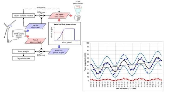
The theoretically predicted power generation (P_predicted) is calculated by substituting the effective wind speed (V_eff) into the performance curve of the Mitsubishi MWT-1000A wind turbine (Figure 6). ‘Power output deficit’ (dP) refers to the difference between predicted and actual (P_SCADA) power generation in a 10 min average.

$$dP=P_{predicted}-P_{SCADA}$$

(5)

(4)

Statistical outliers that are not included within 95% of the statistical distribution of the 10 min average power output deficit were eliminated. Note that the special care is needed when treating outliers if there were power curtailments. In this study, there was no power curtailment and non-operating period (P_SCADA ≤ 0) were excluded.

In addition, data other than the 285–0° and 0–35° sectors were also excluded. Figure 7 shows surface roughness length distribution around the LiDAR location where the disturbed wind directions due to wind turbine tower shading, wake zone, and topographic effect are identified [22]. The reason behind the selection of northerly winds (285–0° and 0–35°) only was to single out only sea breeze cases that can exclude influence factors due to wake and terrain features.

The surface roughness length (z_o) was calculated by a linear least square method to fit a logarithmic wind speed profile (Equation (6)) to measured wind speed data by LiDAR at 40 m, 70 m, and 100 m heights above ground. In the equation below, $u_{*}$ and κ are the friction velocity and von Kármán constant, respectively.

$$V\left(z\right)=\frac{u_{*}}{\mathsf{\kappa }}ln\left(\frac{z}{z_o}\right)$$

(6)

(5)

Finally, the wind turbine deterioration rate was determined through the slope in the analysis of the monthly average of 10 min averaged power output deficit trend.

4. Results and Discussion

4.1. Derivation of the Nacelle Transfer Function

The curve fitting of the free stream wind speed measured a 10 min average at the hub height of 69 m during the LiDAR campaign and the 10 min averaged nacelle wind speed was conducted using three NTFs, i.e., Equations (1)–(3), thereby determining the fitting coefficients. The curve fitting results showed that the fittings (R²) of C_P-NTF (Equation (1)), C_T-NTF (Equation (2)), and non-linear NTF (Equation (3)) were 0.97, 0.99, and 0.97, respectively, and that C_T-NTF had the best fitting result.

The probability distribution of the 10 min averaged wind speed deficit according to the three NTFs is shown in Figure 8, where the distribution of the wind speed deficit in C_T-NTF was the closest to the normal distribution, as well as showing the smallest variance. Consequently, R² of C_T-NTF was the smallest. The wind speed deficit is the difference between the predicted free stream wind speed calculated by substituting the nacelle wind speed into the NTF and the actual free stream wind speed measured by LiDAR. Finally, C_T-NTF was found to be the best fit function from the evaluation of the curve fit regression and the probability distribution of the deficit (Figure 8).

4.2. Analysis of the Wind Turbine Deterioration Trend

The monthly average of normalized capacity factor ($\overline{C{F}_m}$) is calculated by the following equation [5].

$$\overline{C{F}_m}=\frac{C{F}_m}{\left(P_m/\overline{P_m}\right)}$$

(7)

where m stands for month (1, 2, …, 12), $\overline{P_m}$ and $P_m$ are the monthly average of wind power for a long-term (over 10 years) period and a short-term (wind farm operation) period, respectively. In this study, wind power is calculated by hourly wind speed at the hub height from MERRA-2 data, i.e., $P=\frac{1}{2}\rho V^{3}A$ (A: rotor area).

The rate of performance aging is +0.47%p per year when wind resource variability is not considered and this positive rate does not make sense. However, the rate becomes −0.01%p per year when wind resource variability is corrected with 10 year reanalysis data. Moreover, the rate becomes −0.11%p per year when 35 year MERRA-2 data is used as shown in Figure 9. Consequently, it is conjectured that the short-term capacity factor data would not be appropriate when estimating the performance aging rate of wind turbines, even if the wind resource variability were to be corrected with the highly accurate reanalysis data. The sinusoidal pattern that appears every 12 months in Figure 9 is due to the seasonal variation of synoptic wind speeds in Korea, i.e., the strongest in winter and the weakest in summer. Along with wind speed changes, diurnal variations of atmospheric stability by season makes the difference of power output even larger.

Figure 10 is a graph representing the monthly trend analysis of the power output deficit. The power output deficit shows one-year cycle of seasonal variability but a steady increasing trend is obvious. In other words, as performance deteriorated, the difference between theoretical and actual power generation tended to increase linearly. The slope of the trend analysis line in the monthly average of power output deficit for four years is 0.43 kW/month, which can be converted to an output reduction rate of −0.52%p per year (i.e., the rate of deterioration of the capacity factor). One of the reason of seasonal variation would be different wind shear patterns by season in Monsoon climatology.

For reference, the average slope of trend analyses of 1-, 2-, 3-, and 4-year periods was 0.46 ± 0.15 kW/month which is a 6.5% difference (1-year period means each of the four years such as 2009, 2010, 2011, and 2012; 2-year period refers to consecutive two years such as 2009–2010, 2010–2011, and 2011–2012).

The monthly trend analysis without applying the NTF showed the same slope of 0.43 kW/month (R² = 0.77). However, the power output deficit decreased from 85.5 ± 5.4 kW to 41.3 ± 2.9 kW after applying the NTF, resulting in a reduction in both of the mean and the variance for four years by half. In spite of improving the accuracy of power generation prediction by employing NTF calibration, the effect of NTF calibration was not observed obviously in the trend analysis. This implies that the wind speed deficit and the power output deficit are attributable to independent causes. The wind speed deficit is mainly due to wake effect and nacelle geometry but the causes of power output deficit are not directly relevant to wake effect. However, it should be noted that a NTF would also be aging due to blade erosion but it was not considered in this study.

The rate of performance aging (−0.52%p per year) of the wind turbines at the Shinan wind farm is within the range of −0.48%p per year and −1.0%p per year by month, which are similar to the performance aging rates of onshore wind farms in the UK, US and Canada. Note that this value is limited to the Mitsubishi MWT-1000A wind turbines installed at the Shinan wind farm, whereas the values for the UK, US, Denmark, and Canada are the results of a comprehensive analysis of wind turbines made in Europe with various machine types, production years, and operational periods. However, it is of great significance to quantitatively confirm the performance aging of Asian wind turbines installed in the Asian region. It also supports that the figures are similar to those around the world.

The aging of the wind turbines was presumed to be the result of a gradual deterioration in performance due to mechanical aging, and not the result of sudden aging after a given number of years. The overall trend of performance aging progressed in a linear fashion which was observed in previous studies in the UK, Denmark, and Canada.

According to South Korea’s carbon-neutral plan, the wind energy should supply 70 TWh of electricity by 2050, and the wind turbine capacity of 24.6 GW is expected to be installed. However, when considering the performance aging of −0.5%p per year, 1.8 GW should be added to the total capacity (+7.3%). This means that accurate prediction and analysis of the performance aging of wind turbines is not only necessary for the development of control strategy, but is also a significant research field to accelerate carbon neutrality.

5. Conclusions

The reliability of the method of estimating the rate of performance aging in existing wind farms was somewhat low due to the uncertainty of wind resource variability, when applied to wind farms with a short total operating period, i.e., less than 5 years. To overcome this problem, the difference between predicted and actual power generation using SCADA data, which is a monthly average of power output deficit, was calculated, and the rate of performance aging was estimated using a trend analysis.

The main conclusions of the study are summarized as follows:

(1)

The trend analysis of power output deficit at the Shinan wind farm over 4 years showed that the rate of performance aging was –0.52%p per year, and that it progressed linearly. This value was similar to the figure of –0.48%p per year obtained for onshore wind farms in the UK, and −0.54%p per year in the US. This result implies that generally about 10% of performance aging occurs over the 20 years of wind farm operation, and this figure should be reflected when evaluating the cost of wind energy and setting national target.

(2)

It was presumed that the nacelle wind speed is affected nonlinearly depending on the wind turbine’s control mode and related to the performance aging. Despite that the prediction accuracy of wind power output was significantly improved when the nacelle wind speed was corrected using the NTF based on C_T curve, it was found that the performance aging is not directly affected by this correction. Since the wind turbine aging occurs in the mechanical drive, the nacelle wind speed is not affected by the aging of blade control mechanism. Therefore, it is conjectured that the correction using NTF is not mandatory when analyzing the performance aging of wind turbines.

References

1. International Electrotechnical Commission. Wind Turbine, Part. 1: Design Requirement, IEC 61400-1, 3rd ed.; IEC: Geneva, Switzerland, 2005. [Google Scholar]
2. Le, B.; Andrews, J. Modelling wind turbine degradation and maintenance. Wind Energy 2016, 19, 571–591. [Google Scholar] [CrossRef]
3. Hughes, G. The Performance of Wind Farms in the United Kingdom and Denmark; Renewable Energy Foundation: London, UK, 2012; 48p. [Google Scholar]
4. Bach, P.F. Capacity Factor Degradation for Danish Wind Turbines; Paul-Frederik Bach Consulting: Switzerland, 2012; 4p. [Google Scholar]
5. Harrison, J. Economic Analysis of the Algonquin Power Company Amherst Island Wind Energy Generation System; Association to Protect Amherst Island: Amherst Island, ON, Canada, 2013. [Google Scholar]
6. Staffell, I.; Green, R. How does wind farm performance decline with age? Renew. Energy 2014, 66, 775–786. [Google Scholar] [CrossRef] [Green Version]
7. Byrne, R.; Astolfi, D.; Castellani, F.; Hewitt, N.J. A study of wind turbine performance decline with age through operation data analysis. Energies 2020, 13, 2086. [Google Scholar] [CrossRef] [Green Version]
8. Astolfi, D.; Byrne, R.; Castellani, F. Analysis of wind turbine aging through operation curves. Energies 2020, 13, 5623. [Google Scholar] [CrossRef]
9. Hamilton, S.D.; Millstein, D.; Bolinger, M.; Wiser, R.; Jeong, S.G. How Does Wind Project Performance Change with Age in the United States? Joule 2020, 4, 1–16. [Google Scholar] [CrossRef]
10. Shin, D.H.; Ko, K.N.; Huh, J.C. A study on method for identifying capacity factor declination of wind turbines. Int. J. Environ. Ecol. Eng. 2015, 9, 55–59. [Google Scholar]
11. Kim, H.G.; Jang, M.S.; Ko, S.H. Long-term wind resource mapping of Korean west-south offshore for the 2.5 GW offshore wind power project. J. Environ. Sci. Int. 2013, 22, 1305–1316. [Google Scholar] [CrossRef]
12. Ministry of Trade, Industry and Energy. New & Renewable Energy Statistics 2019; Korea Energy Agency: Seoul, Korea, 2020.
13. Kim, H.G.; Jeon, W.H.; Kim, D.H. Wind resource assessment for high-rise BIWT using RS-NWP-CFD. Remote Sens. 2016, 8, 1019. [Google Scholar] [CrossRef] [Green Version]
14. Kim, H.G.; Meissner, C. Correction of LiDAR measurement error in complex terrain by CFD—Case study of the Yangyang pumped storage plant. Wind Eng. 2017, 41, 226–234. [Google Scholar] [CrossRef]
15. Kim, H.G.; Kim, J.Y.; Kang, Y.H. Comparative evaluation of the third-generation reanalysis data for wind resource assessment of the southwestern offshore in South Korea. Atmosphere 2018, 9, 73. [Google Scholar]
16. International Electrotechnical Commission. Wind Turbines—Part 12-2: Power Performance of Electricity Producing wind Turbines Based on Nacelle Anemometry; IEC 61400-12-2; IEC: Geneva, Switzerland, 2008. [Google Scholar]
17. Kim, H.G.; Kang, Y.H.; Yun, C.Y. Derivation of nacelle transfer function using LiDAR measurement. Trans. Korean Soc. Mech. Eng. A 2015, 39, 929–936. [Google Scholar] [CrossRef] [Green Version]
18. Kim, H.G. Method of calibration of nacelle anemometer using LiDAR measurements. In Korea Patent, 10-1383792; Korea Institute of Energy Research: Daejeon, Korea, 2014. [Google Scholar]
19. Ormel, F.T.; Donth, A.; Siebers, T.; Faucherre, C.; Luetze, H. Correction method for wind speed measurement at wind turbine nacelle. In European Patent, 1793123B1; GE International Inc.: Munich, Germany, 2016. [Google Scholar]
20. Martin, C.M.; Lundquist, J.K.; Clifton, A.; Poulos, G.S.; Schreck, S.J. Atmospheric turbulence affects wind turbine nacelle transfer functions. Wind Energy Sci. 2017, 2, 295–306. [Google Scholar] [CrossRef] [Green Version]
21. Burton, T.; Jenkins, N.; Sharpe, D.; Bossanyi, E. Wind Energy Handbook, 2nd ed.; John Wiley & Sons, Inc.: Hoboken, NJ, USA, 2011; ISBN 978-0-470-69975-1. [Google Scholar]
22. Castellani, F.; Astolfi, D.; Mana, M.; Piccioni, E.; Becchetti, M.; Terzi, L. Investigation of terrain and wake effects on the performance of wind farms in complex terrain using numerical and experimental data. Wind Energy 2017, 20, 1277–1289. [Google Scholar]
Figure 1. Total wind turbine installation capacity in South Korea.
Energies 14 02319 g001
Figure 2. Location (left) and layout (right) of the Shinan wind farm (the wind turbines and the LiDAR).
Energies 14 02319 g002
Figure 3. Comparison of the daily-mean wind speed between SCADA and LiDAR data at the hub height.
Energies 14 02319 g003
Figure 4. Wind frequency roses at the Shinan wind farm from 30 November 2009 to 17 March 2010. (a) LiDAR measurement (dashed line: mean wind speed at 70 m above ground); (b) MERRA-2; (c) MERRA-2 over a period of 10 years.
Energies 14 02319 g004
Figure 5. Schematic diagram of analysis of rate of deterioration of performance of a wind turbine.
Energies 14 02319 g005
Figure 6. Power curve, power and thrust coefficient of the Mitsubishi MWT-1000A.
Energies 14 02319 g006
Figure 7. Rose diagram of the surface roughness length around the LiDAR location.
Energies 14 02319 g007
Figure 8. Statistical distributions of 10 min averaged wind speed deficits by NTFs.
Energies 14 02319 g008
Figure 9. Trend analysis of wind turbine deterioration rate by normalized capacity factor with the correction of wind resource variability. (●: monthly capacity factor, black and blue lines: harmonic regression with 95% confidence limits, dashed line: linear regression).
Energies 14 02319 g009
Figure 10. Trend analysis of wind turbine deterioration by monthly average of power output deficit with the CT-NTF correction. (●: power output difference, ■: standard deviation, black and blue lines: harmonic regression with 95% confidence limits, dashed line: linear regression).
Energies 14 02319 g010
Publisher’s Note: MDPI stays neutral with regard to jurisdictional claims in published maps and institutional affiliations.