1. Introduction
The rise of photovoltaic (PV) systems in distribution networks has increased the stochastic generation uncertainties that must be analyzed for power system operation and planning. The PV systems are spatially distributed, and they are mostly correlated with respect to the meteorological uncertainty. This implicates PV systems’ active power as correlated random variables exhibiting different distributions, and proper methodology is required to manage these correlated uncertainties.
The power flow analysis of a network with particular operating conditions is called deterministic load flow (DLF) analysis. The different uncertainties present in the network due to generators, load variations and changes in network configuration are not considered in DLF analysis [
1]. The injection of power into the network by photovoltaic (PV) generators distributed along the feeders represents a relevant source of uncertainty. To consider the above uncertainties, Probabilistic Load Flow (PLF) analysis is useful [
2,
3]; it is mix of DLF and mathematical methods to define uncertain sources, e.g., through their probability density functions (PDF). In this work, the PLF analysis was conducted by considering the correlations among the active power variables of the PV generators.
There are three types of PLF computational methods available. The Monte Carlo (MC) simulation belongs to the first type called numerical methods [
2,
4]. The other two methods are analytical and approximation methods [
5]. Analytical and approximation techniques can accelerate PLF analysis compared to the MC method.
The PLF techniques are very diversified and every methodology among them has its own benefits. Classifications of these methodologies with pros and cons are reported in the following review papers [
4,
5]. However, among the many techniques, the MC simulation remains the reference method, since it delivers the most reliable results and can handle parameters with nonstandard distributions [
6]. For those reasons, the MC simulation is the method adopted in this article. A MC simulation requires a large input sample, and it is obtained using the PDF of the element of interest [
7]. In our case it is the active power of the PV generators.
In some cases, while modeling the uncertainties associated with the PV system, the active power PDF of the PV system is approximated by standard statistical distributions. In [
8] the PV power output was fitted to a bi-modal normal distribution; in [
9] PV power production was modeled by taking the clear sky index model and the data were fit to a beta distribution.
Many other modeling techniques are reported in [
5,
10,
11,
12]; these are solar irradiation and weather approximation-based modeling techniques. They definitely include the meteorological uncertainty, but other factors such as power delivery interruption due to device failure, change in network topology and load unavailability are ignored. To consider these factors in the uncertainty quantification of a PV system, a data-driven approach was used in this work [
13]. When the measurement data of a PV system are analyzed, the PDF of the active power delivered by the PV system shows a complex shape, and it does not fit any standard statistical distribution. In this case, a large set of PV samples for MC simulations were generated by determining the empirical cumulative distribution function (CDF) of measurement and using an inverse sampling method that matched the original distribution [
14].
In the case of multiple PV generators, there exists a correlation among the measurement variables. If the dependence among these variables is ignored and the inverse sampling method is used, the output results can be quite inaccurate. Hence, considering this correlation while generating the samples for an MC simulation is crucial. Known techniques for handling correlations are copulas [
15] and the Gaussian mixture model [
16]. In this article, the investigation is performed by considering a Gaussian copula.
The main contribution of this paper is a PV statistical modeling strategy that combines the information available from historical measurement data with the application of a Gaussian copula to generate samples for further MC simulations. This methodology, which is able to include a PV correlation in a realistic way, was applied to two different test networks, having different loading and balance conditions. Important critical features in the network’s behavior, such as overvoltage and voltage imbalances, were simulated by considering the correct correlation among PV generators, and then making a comparison with the case wherein said correlation is neglected. The organization of this article is as follows: The PLF analysis and three phase unbalanced power flow equations are given in
Section 2.
Section 3 describes the modeling of the PV generation uncertainties using the inverse CDF method and a Gaussian copula.
Section 4 details the test networks employed in this work.
Section 5 explains the simulation framework and comments on the results. Conclusions are given in
Section 6.
2. Probabilistic Load Flow and Voltage Unbalance
PLF analysis consists of including stochastic uncertainties in deterministic load flow simulations followed by a probabilistic interpretation of the resulting network variables [
6]. In DLF problems, the known parameters are the real and reactive power of the loads, and the real power and voltage magnitude of the generators. The analysis is to determine current injections at the buses with their complex voltages. Referring to an electrical network with N buses linked using
l lines, the current and voltage relationship is described by Equation (
1) [
17]; the three-phase unbalanced system complex power equations are also referred to in [
18].
where
| Three phase current; |
| Admittance matrix; |
| Three phase voltage. |
| Current injected in bus |
| Phase representation |
| Element of admittance matrix |
| Combination of buses |
| Combination of phases |
| Complex voltage of bus |
For any bus
i and phase
p, the current
of the bus is given by the Equation (
5).
The complex power of a unbalanced three phase system is given in Equation (
6). Since the complex power term at the left-hand-side is present, the solution results in the voltage of the selected bus under investigation.
where
| Complex power injected; |
| Admittance conjugate; |
| Voltage conjugate. |
The statistical uncertainty present in the power network can be described mathematically by a set of stochastic parameters
where each
represents a random variable with PDF
. In general, such stochastic parameters might be voltage, currents or power injections; more specifically, in this work we focus on the case where the uncertain sources include the active power injected by PV generators normalized to the installed capacity, as is described in
Section 3.
The actual power delivered by a PV generator at different times of the day (e.g., at different hours) changes and it changes its statistical distribution. This uncertainty in active power delivery can be modeled with stochastic parameters whose PDFs depend on time, i.e., , and evaluated numerically starting from measurement data grouped for each time of the day.
Thus, with the dependence on the time and the vector of uncertainty , the voltage of the node’s phase is represented as . For each time , an MC simulation is conducted by generating a large set of uncertainty vector realizations , where . For every vector element , load flow is conducted to determine .
In a three-phase unbalanced system, the network voltage quality is measured by the inequality in its phases; it is called voltage unbalance and is expressed in a percentage as the voltage unbalance factor (
VUF)%. It is defined as the ratio of the negative voltage sequence to the positive voltage sequence component as given in Equation (
7).
where
| Negative voltage sequence component; |
| Positive voltage sequence component; |
| Line voltages; |
| ; |
| . |
3. Modeling Photovoltaic Generation Uncertainties
Power generation using PV modules is highly uncertain because of variable atmospheric conditions. Probabilistic techniques for modeling uncertainties arising from irradiation availability and meteorological effects [
5] do not consider uncertainty caused by partial shading, power network and topology uncertainties due to elemental failure in the device present in the PV system.
To overcome such limitations, in this paper, a data-driven modeling approach based on historical measurement data is considered that can include system-dependent uncertainties.
The proposed methodology is general; however, for illustration purposes we used the real measured and recorded dataset [
19] of active power delivered by some domestic photovoltaic systems in the Sydney power distribution grid.
As an example, the active power levels delivered in a day by three spatially separated PV generators are given in
Figure 1. The PV power delivery data were samples recorded every 30 min and observed for one calendar year. Significant variation in power was observed in mid-day hours.
For such reasons, PV power data have been grouped for different hours of the day representing the sample times . The hourly PDF of the active power variable extracted in the measurement data shows complex shapes and cannot be fit into any standard statistical distributions.
Figure 2 shows the PDFs of the normalized active power for 12:00 p.m. and 3:00 p.m. hourly time windows.
In order to generate a large set of samples distributed according to such a nonstandard distribution as required by Monte Carlo simulations, we followed two different modeling approaches.
The first one was very immediate and assumed that the power levels delivered by two or more PV generation systems were independent random variables. In this case, the well known inversion method for generating samples using the cumulative distribution (CDF) could be directly applied. As a matter of fact, depending on the installation locations, the power levels produced by PV generators are not independent, so it is necessary to consider their correlation while generating samples. In the second and more realistic modeling approach, the Gaussian copula method was utilized to produce correlated samples for MC simulations.
3.1. Inverse CDF Method
It is a method in which the correlation among the random variables, i.e., the correlation among the generators’ active power levels, is not considered. The samples for MC simulations were generated independently; hence, from now on, this method is called the independent method. The PV power generation analysis is done on an hourly basis. The normalized active power delivered by a single PV power generator is considered, and it is represented by a random variable “X” obtained as given by Equation (
10).
where
| X | Normalized active power; |
| Measured active power from the dataset; |
| Installed capacity of the PV generator. |
The random variable
X represents one of the statistical parameters, e.g.,
. For each time sample
, the distribution of
X derived from data is nonelementary and its PDF is given by
. The related CDF
can be deduced numerically from
. The inverse method consists of drawing random numbers from a uniformly distributed variable
that are given in input to the inverse CDF
. This will provide the sample values
x of the random variable X as given in Equation (
11).
For each realization , the related active power is then computed. The same process is repeated, independently, for a second statistical variable , which is supposed to scale a second PV generator, and so on for any other further ones. Finally, the calculated PV power levels are employed as an input to the DLF simulation to get the associated .
3.2. Gaussian Copula
In the second approach, the correlation among different PV generators is extracted from the data using Gaussian copula. The copula is the entity or the function that contains dependence information about the random variables; it joins or couples the uni-dimensional marginal distributions. Copulas are used to model the dependence between two or more random variables, where the marginal distributions of random variables are combined to arrive at a joined distribution. The dependence relations among the marginals are investigated in a common domain, and once the joined distribution is obtained, the random variables are further traced back to their original forms using CDFs without any loss of the information associated. With this, the number of samples required for MC simulation is obtained.
Consider two random variables
X and
Y, with marginal PDFs
and
; the related CDF are denoted as
and
respectively. The aim is to find the joint cumulative distribution
. Using Sklar’s theorem, the copula function with the dependence can be applied to the joint CDF of these random variables. To arrive at the joint CDF, Equation (
12) is used.
where
| Joint CDF of variables X and Y; |
| C | Copula function with dependence; |
| CDF of variable X; |
| CDF of variable Y. |
The correlation between the random variables X and Y can be measured by their correlation coefficient
that is estimated from data samples as given in Equation (
13).
where
| Correlation coefficient; |
| Random variables; |
| N | Number of scalar observations; |
| Standard deviation; |
| Mean. |
The value of lies between −1 and 1; if is 1 then the correlation among the variables is maximum with positive dependence; i.e., the PV generating stations deliver identical power output. If is −1 then the correlation among the variables is maximum with negative dependence; 0 results in no correlation—the PV generating stations result in power output randomly without any dependence.
In order to get desired samples
x and
y with the specified correlation and marginal distributions, a bi-variate normal (Gaussian) distribution [
20] with the correlation
is considered. Samples
and
drawn according to such a bi-variate Normal distribution are fed to the uni-variate Gaussian cumulative distribution
which gives uniformly distributed values
and
. Using
u and
v we can trace back the samples of
x and
y by evaluating the inverse cumulative distribution function, i.e.,
and
.
The data-driven computational flow of the Gaussian copula is summarized in
Figure 3.
As a result, the Gaussian copula allows generating a large set of data samples with prescribed statistical distributions and dependency information as extracted by measurement data. It is important to focus on the fact that using the copula method is more accurate for reconstructing the joint distribution than considering its generation using two independent distributions. For example,
Figure 4 reports the scatter plots of the datasets (for one hour, i.e., 12:00 p.m. to 01:00 p.m.) of two PV generators, along with the samples generated using the Gaussian copula and the independent method, respectively. Even though the marginal PDFs employed in the two techniques were exactly the same (e.g., the marginal PDF shown in
Figure 2), the resulting joint distributions are different, since the Gaussian copula accounts for the correct correlation among the measurement data but the independent method does not. In fact, due to the correlation, the data tend to concentrate along the diagonal line in the
plane, and this behavior is correctly reproduced by the samples generated by the Gaussian copula.
4. Test Networks
The proposed methodologies were implemented in two different test networks having different characteristics for the validation of results [
21,
22]. In both cases, we considered the network’s original configuration and added some uncertain PV generators and statistical user loads. The PV-related uncertainties are represented with two stochastic parameters
and
, which were correlated using the copula method. The nonstandard statistical distributions (e.g., those reported in
Figure 2) of PV-related parameters were extracted from measurement data as described in
Section 3. Besides, four stochastic parameters
were used to scale the maximum active power absorbed by four loads in the nets following the method previously presented in [
23]. Such load-related stochastic parameters are independent and beta distributed (with parameters a = 1.1 and b = 22). On the whole, the uncertainty vector
consists of six statistical parameters.
The test networks used in this work were the following:
The positions of the PV generators and additional loads were assigned by considering a criteria of PV penetration, which is defined as the ratio of the PV capacity to the total installed load capacity of the test network [
24]. In the following, we describe the main characteristics of the considered network.
4.1. IEEE 13 Bus Test Feeder
The 13 bus test feeder provided by IEEE [
21] is of radial type that operates at 4.16 kV. Its phases operate at different voltages, and hence it is an unbalanced network that attracts many researchers. It is heavily loaded for 4.16 kV feeder; the transmission lines come with overhead and underground line types. The loads are classified as spot loads and distributed loads. More details on the network and its elements can be found in [
14,
21]. The network is modified by adding two single-phase PV generators to phase B of bus 3 and bus 4, and four single-phase loads connected to buses 3, 4, 9 and 11, as shown in
Figure 5.
4.2. Non-Synthetic European Low Voltage Test Network
It is a test network modeled using real measurement data, representing a real European town [
22]. The rated voltage is 416 V phase with a 50 Hz phase. It has a 4-wire system design that is isolated, neutral on customer grounds. It consists of 10,290 buses, to which 8087 loads are connected with 30 distribution transformers representing a European-style distribution network. The loads are modeled with load shapes captured using real measurement data. Two PV generators are connected to phase C of bus—1279 and 1284 loads each, as shown in
Figure 6. The loads are connected to phase a and phase C of nodes 1279 and 1283.
5. Simulation Framework and Results
The two test networks described in the previous
Section 4 were modeled in openDSS, and MC simulations were used to evaluate the impacts of the six uncertainty parameters collected in a vector
. In particular, PV uncertainty was reproduced in simulations that started from measurement data and used both the inverse method, i.e., assuming PV generators were statistically independent, and the Gaussian copula method. This later allowed accounting for PV generators’ correlation as described in
Section 3. Simultaneously, the load uncertainty was reproduced by a beta distribution (a = 1.1, b = 22). A large set of samples of statistical parameter vectors
, with
were generated according to the joint distribution of parameters in
and related uncertain power samples
, and the networks were evaluated in some node to calculate the voltage distributions and voltage unbalance factor.
5.1. The IEEE 13 Node Test Feeder Network Response
In this case, the correlated PV generators were connected to node 3 and node 4 in phase B, having maximum power delivery ratings of 200 and 250 kW respectively. The subset of uncertainty vector due to the PV ( and ) was obtained hourly from 10:00 a.m. to 05:00 p.m., with 1 h intervals. The distributions were scaled respectively by 200 and 250 kW power delivery at peaks; then the active power stochastic variable and were realized. The uncorrelated statistical loads were connected to nodes 3, 4, 9 and 11; and each of them was modeled using a beta distribution (a = 1.1, b = 22) each of them scaled for a base of 500 kW. The PV data were highly correlated with the correlation coefficient .
In
Figure 7, we show the PDF of voltage at node 3 simulated with MC method starting from the PV data over one hour time intervals (i.e., from 01:00 p.m. to 02:00 p.m.) using the Gaussian copula and the independent method. It can be observed how the Gaussian method, which accounts for the actual correlation among PV generators, resulted in a wider variability of node voltage (i.e., standard deviation of ≈23 V) compared to the independent method (i.e., standard deviation of ≈17 V). In other words, conducting simulations using data that exhibit a correlation without using a method to handle correlation, such as the one proposed in this article, runs the risk of arriving at incorrect solutions.
In
Figure 8, we report the hourly voltage distribution, from 10:00 a.m. to 05:00 p.m., of voltage at node 3 phase B simulated with the MC method and Gaussian copula. The voltage distribution has 2.38 kV as the minimum and 2.52 kV as the maximum point in the distribution; the large variation of the distribution is seen during the midday hours.
The
of node 3 due to the power injection of highly correlated PV generators is shown in
Figure 9; the percentage voltage unbalance varies from
to
.
Finally, in
Figure 10 we report the comparison among mean values and the standard deviations of the voltage and VUF at the node 3 phase B calculated using the independent method and Gaussian copula. It can be noted that the distribution of voltage and
contains similar mean values, but the standard deviation of the distributions is higher when we model the PV uncertainty with Gaussian copula. It is because the inclusion of the correlation will cause a wide range of distribution; hence we can see more variability in the dispersion of voltage values.
5.2. The Non-Synthetic European Low Voltage Test Network Response
In this test network, we wanted to analyze what happens to a large network when considering correlated PV sources. The PV generators were connected to phase C of nodes 1279 and 1284, with maximum power delivery ratings of 53 and 60 kW respectively. The uncertainty elements related to the PV (
and
) were obtained for every hour from 10:00 a.m. to 05:00 p.m. and were scaled for 53 and 60 kW power delivery at peaks; then the active power stochastic variables
and
were realized. The non-correlated loads were modeled using the beta distribution (a = 1.1, b = 22) and connected to phase A and phase C of nodes 1279 and 1283. The scaling factor of the loads was 30 kW for node 1279 and 20 kW for node 1289. In
Figure 11 we report as an example the voltage distribution in phase C of node 1279, for a one-hour interval from 01:00 p.m. to 02:00 p.m. The voltage varied within the range of 225 to 253 V. Additionally, in this case the generation of a joint distribution can overestimate the peak and underestimate the standard deviation.
For each hour from 10:00 a.m. to 05:00 p.m., the voltage distribution of phase C of node 1279 is given in
Figure 12. The
of node 1279 due to the power injection of highly correlated PV generators and beta distributed loads connected is shown in
Figure 13; the percentage of voltage unbalance varies from
to
.
In
Figure 14 we compare the mean values and standard deviations of the voltage and VUF at node 1279.
6. Conclusions
A data-driven approach for the statistical modeling of PV generation uncertainties was provided in this work; the main aim was to include the dependence information among the measurement data while generating the samples for the MC simulation. To achieve that goal, the Gaussian copula was used to generate a large set of samples that could be used for MC simulations while including the correct dependence information among the samples generated. We demonstrate that the proposed method reconstructs the joint distribution in a better way than using the independent method. By applying the method to the test cases, we proved that the incorrect modeling of correlated data could generate incorrect solutions. This approach was compared to the case where the MC simulation was done while neglecting the correlation among PV generators. Two power networks with different sizes, configuration and complexities were employed to test the hypothesis.
The results clearly show that considering the correct dependence among PV generators data significantly varies the numerically predicted statistical distributions of network voltages and of important figures of merit, such as the voltage unbalance factor. More specifically, MC simulations with correlated PV generators result in a much wider variability of node voltages compared to MC simulations, when the correlation among PV generators is not included. The proposed methodology was applied to PV sources in this article, but in general, it can be applied to other sources, such as correlated wind generators and correlated loads in the PLF studies.
Author Contributions
Conceptualization, H.P., P.M. and G.G.; methodology, P.M. and G.G.; software, H.P. and P.M.; validation, H.P., P.M. and G.G.; investigation, H.P., P.M. and G.G.; writing—original draft preparation, H.P., P.M. and G.G.; writing—review and editing, H.P., P.M. and G.G.; supervision, P.M. and G.G. All authors have read and agreed to the published version of the manuscript.
Funding
This research received no external funding.
Data Availability Statement
Conflicts of Interest
The authors declare no conflict of interest.
References
- Zio, E.; Piccinelli, R.; Delfanti, M.; Olivieri, V.; Pozzi, M. Application of the load flow and random flow models for the analysis of power transmission networks. Reliab. Eng. Syst. Saf. 2012, 103, 102–109. [Google Scholar] [CrossRef]
- Chen, P.; Chen, Z.; Bak-Jensen, B. Probabilistic load flow: A review. In Proceedings of the 2008 Third International Conference on Electric Utility Deregulation and Restructuring and Power Technologies, Nanjing, China, 6–9 April 2008; pp. 1586–1591. [Google Scholar]
- Gruosso, G.; Gajani, G.S.; Zhang, Z.; Daniel, L.; Maffezzoni, P. Uncertainty-aware computational tools for power distribution networks including electrical vehicle charging and load profiles. IEEE Access 2019, 7, 9357–9367. [Google Scholar] [CrossRef]
- Ramadhani, U.H.; Shepero, M.; Munkhammar, J.; Widén, J.; Etherden, N. Review of probabilistic load flow approaches for power distribution systems with photovoltaic generation and electric vehicle charging. Int. J. Electr. Power Energy Syst. 2020, 120, 106003. [Google Scholar] [CrossRef]
- Prusty, B.R.; Jena, D. A critical review on probabilistic load flow studies in uncertainty constrained power systems with photovoltaic generation and a new approach. Renew. Sustain. Energy Rev. 2017, 69, 1286–1302. [Google Scholar] [CrossRef]
- Gruosso, G.; Netto, R.S.; Daniel, L.; Maffezzoni, P. Joined Probabilistic Load Flow and Sensitivity Analysis of Distribution Networks Based on Polynomial Chaos Method. IEEE Trans. Power Syst. 2019, 35, 618–627. [Google Scholar] [CrossRef]
- Gruosso, G.; Maffezzoni, P.; Zhang, Z.; Daniel, L. Probabilistic load flow methodology for distribution networks including loads uncertainty. Int. J. Electr. Power Energy Syst. 2019, 106, 392–400. [Google Scholar] [CrossRef]
- Warren, J.J.; Negnevitsky, M.; Nguyen, T. Probabilistic load flow analysis in Distribution Networks with distributed solar generation. In Proceedings of the 2016 IEEE Power and Energy Society General Meeting (PESGM), Boston, MA, USA, 17–21 July 2016; pp. 1–5. [Google Scholar]
- Diop, F.; Hennebel, M. Probabilistic load flow methods to estimate impacts of distributed generators on a LV unbalanced distribution grid. In Proceedings of the 2017 IEEE Manchester PowerTech, Manchester, UK, 18–22 June 2017; pp. 1–6. [Google Scholar]
- Kumar, R.; Umanand, L. Estimation of global radiation using clearness index model for sizing photovoltaic system. Renew. Energy 2005, 30, 2221–2233. [Google Scholar] [CrossRef]
- Jamil, B.; Siddiqui, A.T. Generalized models for estimation of diffuse solar radiation based on clearness index and sunshine duration in India: Applicability under different climatic zones. J. Atmos. Sol. Terr. Phys. 2017, 157, 16–34. [Google Scholar] [CrossRef]
- Palahalli, H.; Huo, Y.; Gruosso, G. Modelling of Photovoltaic Systems for Real-Time Hardware Simulation. In ELECTRIMACS 2019; Springer: Berlin/Heidelberg, Germany, 2020; pp. 3–15. [Google Scholar]
- Noruzi, A.; Banki, T.; Abedinia, O.; Ghadimi, N. A new method for probabilistic assessments in power systems, combining monte carlo and stochastic-algebraic methods. Complexity 2015, 21, 100–110. [Google Scholar] [CrossRef]
- Palahalli, H.; Maffezzoni, P.; Gruosso, G. Modeling Photovoltaic Generation Uncertainties for Monte Carlo Method based Probabilistic Load Flow Analysis of Distribution Network. In Proceedings of the 2020 55th International Universities Power Engineering Conference (UPEC), Turin, Italy, 1–4 September 2020; pp. 1–6. [Google Scholar]
- Widén, J.; Shepero, M.; Munkhammar, J. Probabilistic load flow for power grids with high PV penetrations using copula-based modeling of spatially correlated solar irradiance. IEEE J. Photovolt. 2017, 7, 1740–1745. [Google Scholar] [CrossRef]
- Jun, Z.; Shuang, Z.; Feng, G.; Xutao, L.; Hongqiang, L.; Zhiwen, W.; Chen, S. An analytical method for probabilistic load flow using Gaussian mixture model. In Proceedings of the 2016 IEEE International Conference on Power System Technology (POWERCON), Wollongong, NSW, Australia, 28 September–1 October 2016; pp. 1–6. [Google Scholar]
- Sereeter, B.; Vuik, K.; Witteveen, C. Newton power flow methods for unbalanced three-phase distribution networks. Energies 2017, 10, 1658. [Google Scholar] [CrossRef]
- Cortés-Caicedo, B.; Avellaneda-Gómez, L.S.; Montoya, O.D.; Alvarado-Barrios, L.; Chamorro, H.R. Application of the Vortex Search Algorithm to the Phase-Balancing Problem in Distribution Systems. Energies 2021, 14, 1282. [Google Scholar] [CrossRef]
- Australian Grid Solar Home Electricity. Available online: https://www.ausgrid.com.au/Industry/Our-Research/Data-to-share/Solar-home-electricity-data (accessed on 15 January 2021).
- Bishop, C.M. Pattern Recognition and Machine Learning; Springer: Berlin/Heidelberg, Germany, 2006. [Google Scholar]
- IEEE 13 Node Test Feeder Data. Available online: https://site.ieee.org/pes-testfeeders/resources/ (accessed on 15 January 2021).
- Koirala, A.; Suárez-Ramón, L.; Mohamed, B.; Arboleya, P. Non-synthetic European low voltage test system. Int. J. Electr. Power Energy Syst. 2020, 118, 105712. [Google Scholar] [CrossRef]
- Gruosso, G.; Maffezzoni, P. Data-driven uncertainty analysis of distribution networks including photovoltaic generation. Int. J. Electr. Power Energy Syst. 2020, 121, 106043. [Google Scholar] [CrossRef]
- Aziz, T.; Ketjoy, N. PV penetration limits in low voltage networks and voltage variations. IEEE Access 2017, 5, 16784–16792. [Google Scholar] [CrossRef]
Figure 1.
Active power per unit produced in a day by three different PV generators that are geographically separated.
Figure 1.
Active power per unit produced in a day by three different PV generators that are geographically separated.
Figure 2.
The normalized active power PDF of a one hour time window. A change in the shape of distribution is clear when comparing 12:00 p.m. and 3:00 p.m. Such changes can also be observed for other hourly time instants considered from 10:00 a.m. to 5:00 p.m.
Figure 2.
The normalized active power PDF of a one hour time window. A change in the shape of distribution is clear when comparing 12:00 p.m. and 3:00 p.m. Such changes can also be observed for other hourly time instants considered from 10:00 a.m. to 5:00 p.m.
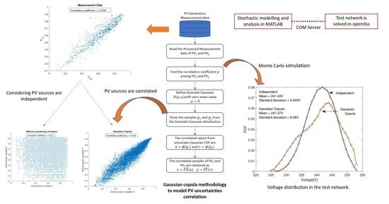
Figure 3.
Schematic representation of the Gaussian copula usage to generate the correlated PV generator samples for the MC simulation.
Figure 3.
Schematic representation of the Gaussian copula usage to generate the correlated PV generator samples for the MC simulation.
Figure 4.
The scatter plots of normalized power levels for two different PV generators obtained using the independent method and the Gaussian copula.
Figure 4.
The scatter plots of normalized power levels for two different PV generators obtained using the independent method and the Gaussian copula.
Figure 5.
The IEEE 13 node test feeder with correlated PV generators connected to 3rd and 4th buses.
Figure 5.
The IEEE 13 node test feeder with correlated PV generators connected to 3rd and 4th buses.
Figure 6.
The modified non-synthetic European low voltage test system network with correlated PV generators.
Figure 6.
The modified non-synthetic European low voltage test system network with correlated PV generators.
Figure 7.
The voltage distribution of node 3 of the IEEE 13 node test network for the one hour time window of 01:00–02:00 p.m.; the active power stochastic variable was modeled considering dependence among the variable using Gaussian copula and the independent method.
Figure 7.
The voltage distribution of node 3 of the IEEE 13 node test network for the one hour time window of 01:00–02:00 p.m.; the active power stochastic variable was modeled considering dependence among the variable using Gaussian copula and the independent method.
Figure 8.
Voltage distribution of node 3 of the IEEE 13 node test network for time window of 10:00 a.m.–05:00 p.m.; the active power stochastic variable was modeled considering the dependence among the variable using the Gaussian copula.
Figure 8.
Voltage distribution of node 3 of the IEEE 13 node test network for time window of 10:00 a.m.–05:00 p.m.; the active power stochastic variable was modeled considering the dependence among the variable using the Gaussian copula.
Figure 9.
of node 3 of the IEEE 13 node test network for the time window of 10:00 a.m.–05:00 p.m.
Figure 9.
of node 3 of the IEEE 13 node test network for the time window of 10:00 a.m.–05:00 p.m.
Figure 10.
Comparison between mean value and standard deviation of voltage at the node 3 (phase B) and the in the case of the independent method and the Gaussian copula.
Figure 10.
Comparison between mean value and standard deviation of voltage at the node 3 (phase B) and the in the case of the independent method and the Gaussian copula.
Figure 11.
Voltage distribution in phase C of node 1279 (PV generator 1) of the non-synthetic European low voltage test network, analyzed using data for a one hour time window, i.e., from 01:00 p.m. to 02:00 p.m., using independent and Gaussian copula methods.
Figure 11.
Voltage distribution in phase C of node 1279 (PV generator 1) of the non-synthetic European low voltage test network, analyzed using data for a one hour time window, i.e., from 01:00 p.m. to 02:00 p.m., using independent and Gaussian copula methods.
Figure 12.
Voltage distribution in phase C of node 1279 (PV generator 1) of the non-synthetic European low voltage test network, analyzed using highly correlated data for all time periods from 10:00 a.m. to 05:00 p.m. using the Gaussian copula.
Figure 12.
Voltage distribution in phase C of node 1279 (PV generator 1) of the non-synthetic European low voltage test network, analyzed using highly correlated data for all time periods from 10:00 a.m. to 05:00 p.m. using the Gaussian copula.
Figure 13.
distribution in phase C of node 1279 (PV generator 1) of the non-synthetic European low voltage test network, analyzed using highly correlated data for all time periods from 10:00 a.m. to 05:00 p.m. using the Gaussian copula.
Figure 13.
distribution in phase C of node 1279 (PV generator 1) of the non-synthetic European low voltage test network, analyzed using highly correlated data for all time periods from 10:00 a.m. to 05:00 p.m. using the Gaussian copula.
Figure 14.
Mean and standard deviation of the voltage distribution of node 1279 phase C and the distribution of the same node in the non-synthetic European low voltage test network, analyzed using the independent method and the Gaussian copula.
Figure 14.
Mean and standard deviation of the voltage distribution of node 1279 phase C and the distribution of the same node in the non-synthetic European low voltage test network, analyzed using the independent method and the Gaussian copula.
| Publisher’s Note: MDPI stays neutral with regard to jurisdictional claims in published maps and institutional affiliations. |
© 2021 by the authors. Licensee MDPI, Basel, Switzerland. This article is an open access article distributed under the terms and conditions of the Creative Commons Attribution (CC BY) license (https://creativecommons.org/licenses/by/4.0/).


