Abstract
Tire normal forces are difficult to measure, but information on the vehicle normal force can be used in many automotive engineering applications, e.g., rollover detection and vehicle and wheel stability. Previous papers use algebraic equations to estimate the tire normal force. In this article, the estimation of tire normal force is formulated as an input estimation problem. Two observers are proposed to solve this problem by using a quarter-car suspension model. First, the Youla Controller Output Observer framework is presented. It converts the estimation problem into a control problem and produces a Youla parameterized controller as observer. Second, a Kalman filter approach is taken and the input estimation problem is addressed with an Unbiased Minimum Variance Filter. Both methods use accelerometer and suspension deflection sensors to determine the vehicle normal force. The design of the observers is validated in simulation and a sensitivity analysis is performed to evaluate their robustness.
1. Introduction
The automotive industry has made significant improvements in vehicle safety and driving performance in the last decades thanks to active control systems. These control systems rely on the measurement and estimation of several parameters and signals such as the wheel slip, sideslip angle. Tire normal forces can also be used to improve the vehicle safety and performance. Indeed, the longitudinal and lateral tire forces are coupled with the wheel loads [1]. Cho [2] showed that the estimate of tire forces, including tire loads, can be used to implement Global Chassis Control (GCC) systems and to further improve vehicle stability. Another practical application of tire normal force estimation is roll-over avoidance and understeering or oversteering prevention [3].
Tire loads are permanently changing when the vehicle is moving. Loads are transferred between wheels during accelerating, braking, and cornering. The position of the center of gravity, the road grade and irregularities on the road also impact the distribution of wheel normal forces making the estimation task a complex problem [4]. Due to the lack of low-cost sensors to measure the vehicle vertical force, a common approach is to consider the normal forces as constant parameters or to use an algebraic expression based on the vehicle longitudinal and lateral accelerations [5]. These open-loop estimation schemes, albeit simple, are not able to give a precise representation of the normal forces.
Doumiati et al. [6,7] provided a cascaded observer to estimate the tire normal forces. The first step of the algorithm estimates the lateral load transfer using a linear Kalman filter from the suspension deflection and accelerometer measurements and an estimate of the vehicle mass. A second observer is then used to infer the normal tire force from the lateral load transfer and a formulation of the normal force algebraic expression with coupling between longitudinal and lateral acceleration. This yields an Extended Kalman Filter. Jiang [8] extended the application of this estimation framework by adding the vehicle pitch dynamics to take in account the road angle and the road irregularities.
Ozkan [9] used a Controller Output Observer (COO) to estimate lateral and normal tire forces. The estimation model is a half-car model which includes the vehicle lateral, heave, roll, and yaw motion. The model does not include pitch dynamics. Moreover, it assumes a constant vehicle velocity and a perfectly flat road. The COO has been successfully used in other automotive applications, e.g., to estimate the vehicle states [10] or to estimate longitudinal tire forces [11].
The goal of the paper is to provide a framework capable of delivering a reliable estimate of the wheel normal forces using low-calibration estimation methods. Contrary to previous work, the estimation of the wheel force will not be derived from algebraic expressions which estimate the normal forces from the vehicle acceleration. Instead, we intend to integrate the suspension dynamics in the normal force estimator to truly capture the tire force generation using suspension deflection sensors and accelerometers. This manuscript also illustrates the application of a recently developed estimation methodology called Youla Controller Output Observer (YCOO). This new approach is compared to the established method for signal estimation: Kalman filtering. Since the estimation problem is not formulated as a state estimation but an input estimation problem, the Unbiased Minimum Variance Filter (UMVF) is used in place of the standard state-estimation Kalman Filter. The comparison between the two estimation methods is based on several criteria: estimation performance, robustness to uncertainties, and ease of design. The performance is evaluated based on simulation results. In these simulations, we cover the major ways normal force can be generated (load transfer, disturbance from the road profile, and inclined road). The robustness is analyzed by conducting a sensitivity study of the suspension parameters, by introducing discrepancies between the estimation model and the simulation model, and by introducing noise in the measurements. Finally, by considering the different requirements to implement the YCOO and UMVF and the different approaches used by each observer (the UMVF uses a stochastic approach in the time domain while the YCOO relies on a deterministic approach in the frequency domain), we aim to highlight that the YCOO estimation framework is easily implementable with a low-calibration burden to guarantee robustness.
The following section analyzes a vehicle model and provides a model that can be used for closed-loop estimation. Section 3 and Section 4 introduce the YCOO and UMVF estimation frameworks. As the normal force estimation is dependent on the vehicle mass estimation problem, Section 5 explains the computation of the vehicle mass estimate, which is used by the two frameworks. Finally, both the YCOO and UMVF are tested in simulation.
2. System Modeling
The generation of vertical forces of a rigid vehicle is linked with the compliance of the suspensions [12]. To develop the estimation frameworks and evaluate the effectiveness, a vehicle model with realistic heave, roll, and pitch dynamics is indispensable. Fortunately, the literature is filled with such vehicle models. Shim [13] described a 14 degrees of freedom vehicle model and validated it against the commercial vehicle models Carsim and ADAMS/Car. Figure 1 shows a schematic of the vehicle model. The degrees of freedom are the longitudinal, lateral, heave, roll, pitch, and yaw motion of the chassis, the vertical dynamics of each unsprung masses, and the wheels spin. The model assumes rigid bodies for the sprung and unsprung masses and neglects the compliance between the chassis and the unsprung mass in the vehicle longitudinal and lateral directions.
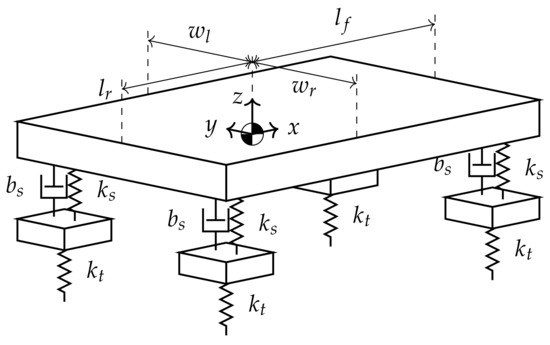
Figure 1.
Fourteen degrees of freedom vehicle model. The x, y, and z axes indicate, respectively, the longitudinal, lateral, and vertical directions of the vehicle. Parameters , , and denote the suspension stiffness, damping, and the tire stiffness.
The model described in Figure 1 gives an accurate representation of the vehicle. However, it is highly complex which limits its usage to implement vehicle observers. Before beginning the observer development, a linear system analysis of the vehicle is performed. Its purpose is to determine the cross-coupling effects between the input–output pairs to facilitate the observer design. The inputs of the model are the tire loads and the outputs are the suspension deflections.
The coupling between input-output pairs of the plant G is analyzed using the Relative Gain Array (RGA) where is the plant gain [14]. Since RGA is a linear analysis tool, the model mapping the tire loads , , and , to the suspension deflections , , , and must first be linearized. The operating point is chosen to be a steady-state cornering such that the vehicle velocity is −1 and the vehicle lateral acceleration is (i.e., the vehicle lateral velocity is −1; the heave velocity is −1; and the roll, pitch, and roll angular velocities are −1 and −1). The matrices and correspond, respectively, to the RGA of a vehicle without an anti-roll bar and with an anti-roll bar on the rear axle. The inputs are .
The matrix is almost equivalent to an identity matrix which indicates that there is almost no coupling between the four corners of the vehicle without anti-roll bar. Concerning the vehicle equipped with anti-roll bar, the two axles decoupled as the bottom left and upper right submatrices of are almost zero. However, the anti-roll bar introduces a coupling between the left and right rear normal loads and , as can be seen in the bottom right corner of .
We assume that the vehicle is not equipped with an anti-roll bar. Thus, the wheel load of each corner of the vehicle can be estimated individually. A simpler model (Figure 2) is introduced to model the suspension of each wheel of the vehicle. The estimation model is a quarter-car model [15] with two inputs: a force applied on the sprung mass to represent the load transfer and another force which represents the tire load. In practice, the anti-roll bar of the vehicle should be considered and the coupling between the left and right normal forces should not be ignored. This coupling would appear as a load transfer from one side to the other when the two wheel loads are not equal, e.g., during cornering. The anti-roll bar would prevent the use of a quarter-car model and require a half-car model.
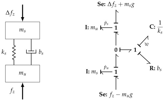
Figure 2.
Quarter-car model of the suspension with wheel normal force and load transfer as inputs.
The bond graph of the model in Figure 2 yields the equation of motion of the quarter-car model
where and are the sprung mass and unsprung mass momentum, is the suspension deflection, is the wheel normal load, represents the load transfer applied to the wheel, is the suspension stiffness, is the damper coefficient, and and are the sprung and unsprung masses of the corner of the vehicle. The states of the model are . It is assumed that the vehicle is equipped with suspension deflection sensors and accelerometers on the sprung mass, hence the measurements are . The model inputs are .
3. Controller Output Observer
The Youla Controller Output Observer, based on the COO framework [9], is a model-based estimation technique that uses a controller to minimize the error between the measurement and the virtual measured signals of an estimation model. Contrary to the Luenberger observer, the YCOO does not assume that all system inputs are known; it is therefore well suited for an input estimation problem. Instead of designing a static gain controller via pole placement similarly to the Luenberger observer, the YCOO uses a dynamic controller designed with Youla parameterization [16]. This technique allows including information about the sensor dynamics and its noise content in the frequency domain to ensure good robustness and performance. A block diagram of the estimation concept is given in Figure 3. Measurements y are fed to the YCOO to provide an estimate of the signal u. The YCOO is decomposed into two components: an estimation model that maps the estimated signal to the virtual measurement and a controller that is responsible to follow those measurements [17].
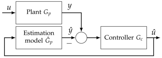
Figure 3.
Block diagram of the YCOO estimation concept.
The transfer function from the the true signal u and the estimated signal is given by where is the return ratio. If there is no discrepancy between the estimated plant and the actual one (), then this transfer function corresponds to the closed-loop transfer function . If the plant has multiplicative uncertainty such that , the relation becomes where Y is the Youla transfer function. This shows that the YCOO relies on an accurate model of the system. Indeed, to guarantee good tracking of the measured quantities, is needed at low frequencies. This condition on also constrains the gain of Y to the inverse of the plant gain at low frequencies since . If the model is not correct, however, the term introduces a steady-state error that cannot be compensated by the observer unless the plant gain is very high at low-frequency. Moreover, for the nominal system , the transfer function mapping the sensor noise to the estimation error is also given by Y. Thanks to its loop shaping approach, the YCOO directly addresses the trade-off between noise rejection, bandwidth, and robustness to high-frequency multiplicative uncertainties. Indeed, a higher bandwidth would increase the gain of Y at higher frequency, making the estimation more sensitive to noise and less robust to multiplicative uncertainties.
The quarter-car model described in the last section is used as the estimation model . The Youla parameterization technique is applied to design the controller from the estimation model. The plant model can be written as a transfer function mapping the signals to .
The first step in deriving a controller using the Youla parameterization technique is to find the Smith–McMillan form of the plant such that . The Smith–McMillan form [18] is useful in multi-variable control as it gives a realization of the plant in a basis where the plant is decoupled (i.e., its transfer function matrix is a diagonal matrix). The poles and transmission zeros of the Smith–McMillan form correspond to the poles and zero of the original system and the unimodular matrices and describe the transformation from the original basis to the basis used by the Smith–McMillan form. The Smith–McMillan form of the plant and its unimodular matrices and are
The controller is designed such that the decoupled system is a second-order Butterworth filter of unit gain with additional poles to make the controller proper, see Equation (8). The damping ratio is set to as it offer good trade-off between fast transient and small oscillations. A large enough bandwidth is necessary for the wheel load estimate to be used by the control system. Moreover, the frequency response of a suspension mapping the road disturbance to tire force is shaped as a band-pass filter [12] whose high cutoff frequency is the wheelhop frequency (typically located at 10 ). Thus, to capture the tire force response, the closed-loop bandwidth should be faster than the wheelhop frequency. The controller is designed such that and the bandwidth of the closed-loop system is 30 . Singular values of the closed-loop transfer function and of the controller are given in Figure 4. At frequencies below the bandwidth, is 0 and has low gain, ensuring a good tracking. At higher frequencies, the gain of decreases to reject sensor noise and make the estimate robust against high-frequencies model mismatch.
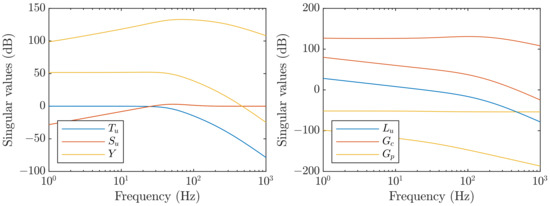
Figure 4.
Singular values of the closed-loop transfer function , , and Y and of the return ratio , , and .
Let such that , the closed-loop transfer function and the controller transfer function matrix is obtained from the following equations which are derived from [17]
This yields the controller
The transfer function from the measured signal y to the estimated input is given
Hence, the estimate of the normal force given by the YCOO is
The same equation can be obtained by combining (3) and (4) and by adding a filter with unit gain. Moschuk et al. [19] patented a concept to estimate wheel normal force using only suspension deflection sensors. The invention uses derivative filters to compute the suspension deflection velocity and the unsprung mass velocity (assuming the sprung mass vertical acceleration is null). It then uses damper and spring force maps to compute the tire normal force. Writing the derivative filter as , the estimation in Reference [19] is
This is similar to the estimate of the wheel normal force given by the YCOO in (15).
4. Unbiased Minimum Variance Filtering
The Unbiased Minimum Variance Filter is a variation of the Kalman filter for systems with unknown inputs. It gives an unbiased (zero-mean error) estimate of the model states and unknown inputs [20] with the assumption that the system is strongly observable. Consider the discrete Linear Time-Invariant (LTI) system
where are the model states, the known inputs, and the unknown inputs. The states and inputs of the estimation model are . The LTI system (17) is strongly observable if the matrix has full column rank [21] ( is the G matrix considering only feedthrough unknown inputs, i.e., with all zero-columns removed).
Since the first column of corresponds to the observability matrix, observability is a necessary condition for strong observability. Unfortunately, the system representing the quarter-car model with unknown force inputs (Equations (2)–(4)) is not observable. Indeed, similarity transformation shows that the state associated to the direction does not produce any observable output. The system is reduced to eliminate the unobservable states. Moreover, it is necessary to use additional measurements to make the system strongly observable. The measured signals used by the UMVF is . Note that suspension deflection sensors such as linear variable transformers which defines an electrical signal based on the position of an objected it is connected to can only measure deflection [22]. The measurement of the suspension relative velocity needed by the UMVF requires differentiating the signal , which requires additional signal processing.
Similar to the Kalman filter, the estimated states is computed in two steps. First, the estimated signals are computed based on the plant model.
Second, the gain is computed to guarantee an unbiased estimate of the model states.
with n the number of states and p the number of unknown input . Given an unbiased estimate , Palanthandalam-Madapusi [23] showed that an unbiased estimate of unknown inputs can be obtained from the following equations
where † denotes the Moore–Penrose pseudo-inverse. Computing the unknown inputs using Equations (27) and (28) guarantees that and , respectively. If H or G have full column rank, then this translates to . In the general case where both H and G are not full column rank, it is necessary to combine Equations (27) and (28) to compute an unbiased estimate . In this article, we propose to compute the unknown input by solving a linear system. Let and be the matrices of left eigenvectors associated to non-zero eigenvalues of and . The unknown input is the solution of:
Without loss of generality, we can assume that , and it is possible to obtain at least p left eigenvectors of and associated to non-zero eigenvalues. Therefore, the matrix has full column rank. Taking the mean of (29) yields
Since the matrix has full column rank, this guarantee that , i.e., is an unbiased estimate of .
5. Vehicle Mass Estimation
Both observers require knowledge of the vehicle mass and the location of the center of gravity. Indeed, the estimate of signals from the observer, as given in (5), directly depends on the vehicle mass. The static wheel load must be added to this estimate to compute the wheel load. This section presents a simple algorithm to obtain the static load of each wheel. More elaborate algorithms could be applied [24].
Algebraic expressions can be used to describe the wheel load distribution in quasi-steady-state.
where the static load and the load transfer terms are
Variables and denote the distance from the center of gravity of the vehicle to the left and ride sides; is the track width; and denote the distance from the center of mass to the front and rear axles; is the wheelbase; m is the total vehicle mass; g is the acceleration of gravity; h is the height of the center of mass; and and are the longitudinal and lateral acceleration due to vehicle acceleration, which also include the gravity component on the vehicle longitudinal and lateral axes.
The vehicle mass estimation algorithm is run when the vehicle is not moving. The wheel load corresponds to the force produced by the suspension deflection ignoring the weight of the unsprung mass. Hence, at steady-state, the wheel load in Equation (31) is replaced by . This yields
where and are the longitudinal and lateral accelerations measured by the sensors and correspond to the acceleration of gravity in those directions if the vehicle is parked on a slope.
This corresponds to a system of four equations with four unknowns, m, , , and h (replacing and by and with l the vehicle wheelbase and w the axle track width). Thus, the position of the center of mass and the vehicle mass can be obtained when the vehicle is not moving.
6. Simulation Results
In this section, the YCOO and UMVF observers developed in Section 3 and Section 4 are tested in simulation. The full-car model shown in Figure 1 is assumed to represent the actual vehicle dynamics and the measured ground-truth signals are extracted from the 14 degrees of freedom vehicle model. The driving scenarios presented aim to cover all possible ways to redistribute tire loads, i.e., longitudinal or lateral load transfer, road irregularities, and sloped road. The results are also compared to the algebraic expression for normal force.
Figure 5a shows the estimates during a braking step of 3000 at 1 from an initial velocity of 90 −1. The two observers provide better estimates than the algebraic expression which suffers from a steady-state error. Moreover, the two observers are intentionally not initialized; both observers converge in approximately . Figure 5b shows the estimate during a double lane change maneuver with a constant velocity of 90 / and with maximum lateral acceleration of . Both estimators provide a good estimate of the tire vertical force, whereas the estimation from algebraic expression does not capture the transient response. Figure 5a,b validates the two estimators for situations where the load transfer is due to longitudinal or lateral acceleration.
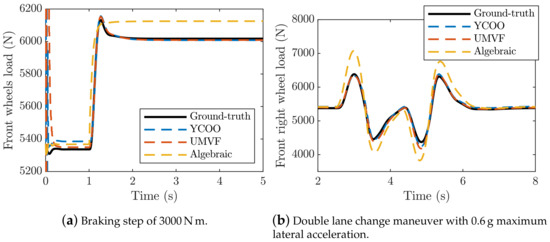
Figure 5.
Vertical tire force estimation on maneuver with longitudinal and lateral only acceleration.
Figure 6 shows the estimate during a bounce sine sweep test. The vehicle velocity is maintained at 20%. The road profile corresponds to sinusoidal bumps of decreasing wavelength with decreasing amplitude. The minimum wavelength is . Thus, the road excites the suspension over the frequency range 0 to 3.5 . The YCOO and the UMVF are able to estimate the wheel loads. Both observers reproduce the frequency response of the suspension: the wheel load amplitude increases when the road excitation get closer to the the suspension frequency ( obtained when ) and remains constant at frequencies between the suspension and wheelhop frequencies. Since the longitudinal and lateral accelerations during this maneuver are almost zero, the algebraic expression is not able to provide an accurate estimation of the wheel loads. The effect of road slope on the estimation scheme is investigated in Figure 7. The vehicle is driven from a flat road to a slope of 20% gradient. The YCOO and the UMVF capture the load transfer due to the road gradient and provide a good estimate during transient.
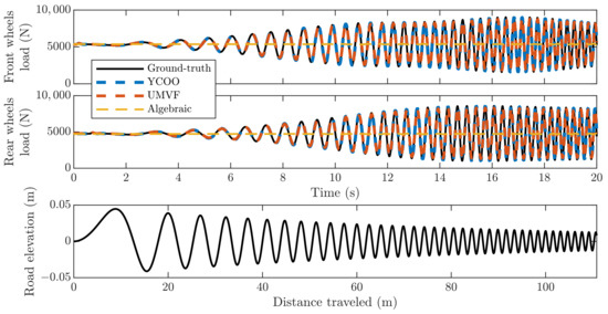
Figure 6.
Vertical tire force estimation during a bounce sine sweep test. Vehicle speed is constant at 20 −1. The minimum wavelength is at %. The bottom figure shows the road profile.
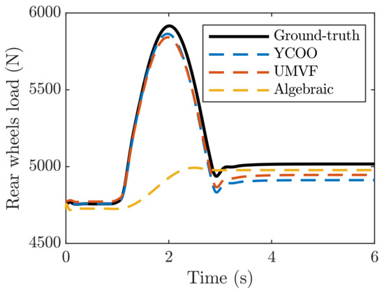
Figure 7.
Vertical tire force estimation when driving on a 20% slope.
It is not practical to assume that the estimation model is a perfect representation of the actual suspension. Figure 8 evaluates the sensitivity of the wheel load estimation against the suspension stiffness. Uncertainties over this parameter result in an offset between the real and estimated wheel load. This is due to the wrong calibration of the mass estimation strategy. The load transfer estimate also suffers from uncertainties in the suspension stiffness. Indeed, without any uncertainty, both observers yield a correct load transfer of 700 , but with a 50% stiffer suspension the load transfer estimate is only 450 . The robustness against the damping coefficient is investigated in Figure 9a. The YCOO and the UMVF provide the same estimate, thus only the estimate given by the UMVF is shown in Figure 9a. The estimation is not robust against the damping coefficient in the transient but it does not affect the steady-state estimation. Similarly, nonlinearities in the damper map affect the transient of the wheel load estimate when the suspension operates in the region approximated by the linear damper map. The linear and nonlinear damper maps are given in Figure 9b.
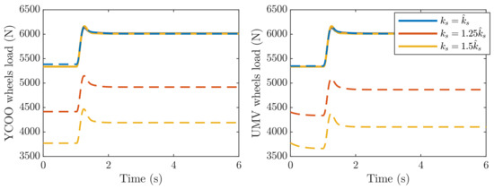
Figure 8.
Robustness against suspension stiffness during a braking maneuver. Solid lines show the ground-truth signals and dashed lines show the estimated ones.
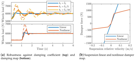
Figure 9.
Robustness against uncertainties in the damping map during a braking maneuver. Solid lines show the ground-truth signals and dashed lines show the estimated ones.
Finally, Figure 10 shows the estimated signals obtained with the YCOO and the UMVF when Gaussian white noise of time correlation 10 and of power spectral density and is, respectively, added to the sprung mass vertical acceleration and to the suspension deflection measurements. The YCOO offers better noise rejection than the UMVF.
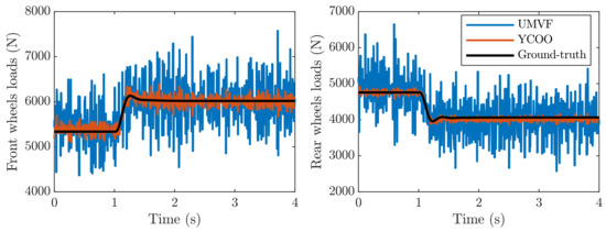
Figure 10.
Estimation with noisy measurements.
7. Conclusions
The estimation of the wheel loads is formulated as an input estimation problem. A quarter-car model with load transfer and tire normal force is used as the estimation model. Two observers are designed. A Youla controller is designed to minimize the error between the measurement and the estimated model output in the Youla Controller Output Observer framework. Similarly, unobservable states of the quarter-car model are removed to use the Unbiased Minimum Variance Filter. Since the design of the YCOO is based on the frequency domain and the closed-loop transfer functions , , and Y, it directly addresses the trade-off among noise rejection, high bandwidth, and good robustness when tuning the observer.
Both observers were tested in simulation and provide good estimates as long as the model possesses a good enough representation of the suspension. Moreover, the anti-roll bar introduces coupling between the two wheels of the same axle. In this case, the quarter-car estimation model cannot be used and should be replaced by a half-car model. Despite using different approaches to solve the input estimation problem and different design methods, both controllers give similar performance and robustness, but the proposed YCOO provides better noise rejection than the UMVF. The YCOO provides a much simpler structure and observer tuning than the UMVF as it does not require the system to be observable and requires only two measurement when the UMVF needs a third measurement with additional signal processing.
Author Contributions
Conceptualization, L.F. and F.A.; methodology, L.F., F.A. and J.V.A.; software, L.F.; validation, L.F. and F.A.; formal analysis, L.F., F.A., and J.V.A.; supervision: M.K. and R.J.; writing—original draft preparation, review and editing: L.F. and F.A.; funding acquisition: F.A. and M.K. All authors have read and agreed to the published version of the manuscript.
Funding
This research was funded under grant Ford Motor Company: AFFORDM.
Institutional Review Board Statement
Not applicables.
Informed Consent Statement
Not applicable.
Acknowledgments
The authors thank Ford Motor Company for its support of this work.
Conflicts of Interest
The authors declare no conflict of interest.
Abbreviations
The following abbreviations are used in this manuscript:
| COO | Controller Output Observer |
| GCC | Global Chassis Control |
| LTI | Linear Time-Invariant |
| RGA | Relative Gain Array |
| UMVF | Unbiased Minimum Variance Filter |
| YCOO | Youla Controller Output Observer |
References
- Chen, W.; Xiao, H.; Wang, Q.; Zhao, L.; Zhu, M. Integrated Vehicle Dynamics and Control; John Wiley & Sons Singapore Pte. Ltd.: Singapore, 2016. [Google Scholar]
- Cho, W.; Yoon, J.; Yim, S.; Koo, B.; Yi, K. Estimation of Tire Forces for Application to Vehicle Stability Control. IEEE Trans. Veh. Technol. 2010, 59, 638–649. [Google Scholar]
- Alatorre, V.A.; Victorino, A.; Charara, A. Estimation of Wheel-Ground Contact Normal Forces: Experimental Data Validation. IFAC PapersOnLine 2017, 50, 14843–14848. [Google Scholar] [CrossRef]
- Doumiati, M.; Charara, A.; Victorino, A.; Lechner, D. Vehicle Dynamics Estimation Using Kalman Filtering: Experimental Validation; ISTE; John Wiley and Sons Inc.: London, UK; Hoboken, NJ, USA, 2013. [Google Scholar]
- Rajamani, R. Vehicle Dynamics and Control; Mechanical Engineering Series; Springer: Berlin/Heidelberg, Germany, 2011. [Google Scholar]
- Doumiati, M.; Victorino, A.; Charara, A.; Baffet, G.; Lechner, D. An Estimation Process for Vehicle Wheel-Ground Contact Normal Forces. IFAC Proc. Vol. 2008, 42, 7110–7115. [Google Scholar] [CrossRef]
- Doumiati, M.; Victorino, A.; Charara, A.; Lechner, D. Virtual Sensors, Application to Vehicle-Tire Road Normal Forces for Road Safety. In Proceedings of the American Control Conference, San Diego, CA, USA, 17 June 2009; pp. 3337–3343. [Google Scholar] [CrossRef]
- Jiang, K.; Pavelescu, A.; Charara, A.; Victorino, A. Estimation of vehicle’s vertical and lateral tire forces considering road angle and road irregularity. In Proceedings of the 2014 17th IEEE International Conference on Intelligent Transportation Systems, ITSC 2014, Qingdao, China, 8–11 October 2014. [Google Scholar] [CrossRef]
- Ozkan, B.; Margolis, D.; Pengov, M. The Controller Output Observer: Estimation of Vehicle Tire Cornering and Normal Forces. J. Dyn. Syst. Meas. Control 2008, 130. [Google Scholar] [CrossRef]
- Velazquez Alcantar, J.; Assadian, F.; Kuang, M. Vehicle Velocity State Estimation using Youla Controller Output Observer. In Proceedings of the 2018 Annual American Control Conference (ACC), Milwaukee, WI, USA, 27–29 June 2018; Volume 2018, pp. 2587–2592. [Google Scholar]
- Velazquez Alcantar, J.; Assadian, F. Longitudinal Tire Force Estimation Using Youla Controller Output Observer. IEEE Control Syst. Lett. 2018, 2, 31–36. [Google Scholar] [CrossRef]
- Jazar, R.N. Vehicle Dynamics: Theory and Application; Springer: Boston, MA, USA, 2008. [Google Scholar]
- Shim, T.; Ghike, C. Understanding the limitations of different vehicle models for roll dynamics studies. Veh. Syst. Dyn. 2007, 45, 191–216. [Google Scholar] [CrossRef]
- Skogestad, S. Multivariable Feedback Control: Analysis and Design, 2nd ed.; John Wiley & Sons: Chichester, UK; Hoboken, NJ, USA, 2005. [Google Scholar]
- Qin, Y.; Wei, C.; Tang, X.; Zhang, N.; Dong, M.; Hu, C. A novel nonlinear road profile classification approach for controllable suspension system: Simulation and experimental validation. Mech. Syst. Signal Process. 2019, 125, 79–98. [Google Scholar] [CrossRef]
- Youla, D.; Bongiorno, J.; Lu, C. Single-loop feedback-stabilization of linear multivariable dynamical plants. Automatica 1974, 10, 159–173. [Google Scholar] [CrossRef]
- Assadian, F.; Mallon, K. Neoclassical Control: Control Systems and Estimation Design using the Youla Parameterization Technique; John Wiley & Sons, Inc.: Hoboken, NJ, USA, 2021. [Google Scholar]
- Chen, C.T. Linear System Theory and Design, 3rd ed.; Oxford University Press, Inc.: Oxford, MS, USA, 1998. [Google Scholar]
- Moschuk, N.; Nardi, F.; Ryu, J.; O’Dea, K. Estimation of Wheel Normal Force and Vehicle Vertical Acceleration. U.S. Patent 8326487, 4 December 2012. [Google Scholar]
- Gillijns, S.; De Moor, B. Unbiased minimum-variance input and state estimation for linear discrete-time systems. Automatica 2007, 43, 111–116. [Google Scholar] [CrossRef]
- Kratz, W. Characterization of strong observability and construction of an observer. Linear Algebra Appl. 1995, 221, 31–40. [Google Scholar] [CrossRef]
- Krauze, P.; Kasprzyk, J.; Kozyra, A.; Rzepecki, J. Experimental analysis of vibration control algorithms applied for an off-road vehicle with magnetorheological dampers. J. Low Freq. Noise Vib. Act. Control 2018, 37, 619–639. [Google Scholar] [CrossRef]
- Palanthandalam-Madapusi, H.J.; Bernstein, D.S. Unbiased Minimum-variance Filtering for Input Reconstruction. In Proceedings of the 2007 American Control Conference, New York, NY, USA, 9–13 July 2007; pp. 5712–5717. [Google Scholar] [CrossRef]
- Rhode, S.; Gauterin, F. Vehicle mass estimation using a total least-squares approach. In Proceedings of the 2012 15th International IEEE Conference on Intelligent Transportation Systems, Anchorage, AL, USA, 16–19 September 2012; pp. 1584–1589. [Google Scholar]


Publisher’s Note: MDPI stays neutral with regard to jurisdictional claims in published maps and institutional affiliations. |
© 2021 by the authors. Licensee MDPI, Basel, Switzerland. This article is an open access article distributed under the terms and conditions of the Creative Commons Attribution (CC BY) license (https://creativecommons.org/licenses/by/4.0/).