Optimal Generation Scheduling in Hydro-Power Plants with the Coral Reefs Optimization Algorithm

Abstract

Hydro-power plants are able to produce electrical energy in a sustainable way. A known format for producing energy is through generation scheduling, which is a task usually established as a Unit Commitment problem. The challenge in this process is to define the amount of energy that each turbine-generator needs to deliver to the plant, to fulfill the requested electrical dispatch commitment, while coping with the operational restrictions. An optimal generation scheduling for turbine-generators in hydro-power plants can offer a larger amount of energy to be generated with respect to non-optimized schedules, with significantly less water consumption. This work presents an efficient mathematical modelling for generation scheduling in a real hydro-power plant in Brazil. An optimization method based on different versions of the Coral Reefs Optimization algorithm with Substrate Layers (CRO) is proposed as an effective method to tackle this problem. This approach uses different search operators in a single population to refine the search for an optimal scheduling for this problem. We have shown that the solution obtained with the CRO using Gaussian search in exploration is able to produce competitive solutions in terms of energy production. The results obtained show a huge savings of 13.98 billion (liters of water) monthly projected versus the non-optimized scheduling.

1. Introduction

Obtaining the optimal generation scheduling in a Hydroelectric Power Plant (HPP) is a challenging problem, with direct implications in the plant’s energy production performance and in the amount of water consumed in the generation process. Generation scheduling is a kind of Unit Commitment (UC) problem [1], i.e., a family of mathematical optimization problems in the electric energy generation, where the production of a set of turbine-generators is somehow managed to achieve a common target, in this case particularized for HPPs. In general, UC problems have some properties such as higher dimensionality, non-linearity, a combinatorial and multimodal nature which are hard to solve efficiently, respecting the existing operational constraints [2]. In the case of generation scheduling in HPPs, it is necessary to have a production modeling for the power generation. The hydro-power plant is composed of turbine-generator units in which each unit needs to deliver part of the total demand dispatched. In this sense, the objective to be achieved is to find the amount of efficient energy that each turbine-generator must generate (in MW) for the system. Thus, the general goal is minimizing the costs and the usage of water resources, whether fulfilling of power demand and respecting the restrictions [3].

Most HPPs have a usual operating mode that works by equally distributing required demand among the ready to use turbine-generators. Nevertheless, note that this equal distribution generally does not lead to an efficient schedule for each turbine-generator, because the generator may not be at its maximum efficiency point. Thus, finding the maximum efficiency point of each turbine-generator set for the generation scheduling problem in HPPs, can be a task considered to be highly complex [4,5]. Research on the optimal operation of electric power systems started around the 1940s [4,6] and, from then, it has been highly influenced by computer science and optimization theory.

In recent decades, different computational techniques and math modelings were proposed to solve problems related to generation scheduling in HPPs. These approaches, took into account that the UC is a NP-hard, non-linear, multi-stage and stringent constraint problem [7]. Optimization models to maximize the power production in short-term hydro-power unit commitment were proposed in [8] to perform the maximum power produced storage for all possible combinations of turbines using Mixed-integer linear programming (MILP). In [9] a proposed study to perform the maximum power produced storage for all possible combinations of turbines was done. These both works solved the UC problem without implementation of penstock losses. This fact has disadvantages for solving the problem as it does not cover the real nature of hydro-power production.

The Linear Programming application [9], Lagrangian multiplier, in which this class of method presents a set of sensitive aspects that often require time-consuming tuning tasks [10], and the Branch-and-Bound with Projected Gradient methods [11] (in which it is not clear how the penstock losses and operational coefficients of turbines were obtained) are also common strategies for solving UC problems to minimize operational costs. These deterministic methods have some advantages as a convergence guarantee, less computational effort, flexible formulation, and not requiring the calculation of second derivatives (in Gradient methods). However, the aforementioned methods have characteristics which are the linearization of the objective functions and the constraints imposed on the problem, which have a non-linear nature, in which this process can cause losses of information and inconsistency in the solutions.

Meta-heuristic approaches have also been applied to obtain the optimal operation of power systems in UC problems, such as Particle Swarm Optimization (PSO) [12] that provided the operation of multi-reservoir system, to minimize the energy shortages with complying with the hydraulic and operational constraints. The Real coded Genetic Algorithm (RGA) was proposed by [13] to make the optimal hydro-thermal scheduling operation reaching a low computing time. The Differential Evolution algorithm (DE) was implemented via the Parallel self-adaptive approach to provide optimal electric dispatch in [14,15]. The study described by [14] indicates that the main goal of the optimization process in UC problems was to satisfy the system demand for 24 h with a decreased usage of water quantity per electrical energy unit reached. In [15] the results shows a significant decreasing trend and extreme flood occurrences in a cascade UC approach.

The non-linear fuzzy methods are addressed by [16] to make a predictive control system in the HPP and the current practice of using machine learning methods to solve the UC problems [17,18]. Some approaches to assess dam releases from hydro-power reservoirs with improving the power production presented solid results using evolutionary algorithms as a solver [19,20]. Combinations of mixed programming with meta-heuristics are addressed in [21], where the goal was to minimize the profit-based in competitive electricity markets. In [22] it has proposed a coupled approach where an Evolutionary Programming is used to optimize the cost functions in a refurbished power grid. Hybrid techniques, such as mixing the Genetic Algorithms, and Differential Evolution have been tested on a generation scheduling problem in an HPP with six turbine-generators [23] showing that this approach achieves competitive results in solving UC problems.

In general, the largest advantage of using meta-heuristics over classical deterministic techniques to solve UC-like problems is that no linearization is required. These techniques allow including non-continuous, non-convex and non-differentiable objective functions, and they have an easy and robust implementation [24,25]. On the other hand, in some modeling of the UC problem these techniques can become computationally expensive. This fact occurs because they are based on a population of potential solutions to the problem [26]. Such methods are efficient in the search for solutions both global and local, being sensitive to the fine-tuning parameters and the possibilities of premature convergence, when the search space increases with respect to the number of generating units of the HPP to be optimized [27].

In this work we solve the generation scheduling problem in a real hydro-power plant. Specifically, we propose a generalist mathematical modeling to calculate hydraulic losses for HPPs. The model was built using real data. From the dataset that was structured by us, the concept of “learning from data” was applied. An approximation of the data was performed via linear regression. This action corroborates the ideas present in machine learning techniques. The realization of this approach minimizes the computational time to obtain optimized solutions via meta-heuristics in the problem of addressing electrical dispatch. Here, our objective is to maximize the power production in an HPP, saving as much water as possible. For this, we are proposing the use of an effective method for solving the generation scheduling in HPPs, by implementing different versions of the Coral Reefs optimization (CRO) [28].

Conceptually, the CRO is an evolutionary-type (meta-heuristic) algorithm that is based on the concept of reproductive behavior of corals on real coral reefs. This algorithm can be considered to be a mix of the Simulate Annealing and Evolutionary algorithms [29]. The CRO algorithm proposed in this work can be tested with different search operators, as exploration mechanisms, obtaining this a powerful evolutionary-like algorithm for solving optimization problems. We have also tested an ensemble version of the algorithm, called CRO-SL, in which all the searching algorithms are included together into a single population, forming an efficient ensemble approach. To our knowledge, this is the first time that the CRO algorithm is applied to solve generation scheduling problems in HPPs, as an optimal system controller of the plant. We show its excellent performance in a real problem, which is considered the generation scheduling of an HPP energy producing in Brazil.

The work structure follows: Section 2.1 presents the problem formulation of the generation scheduling problem in HPPs considered in this work, including a novel mathematical model to operational control of plant taken into account hydraulic losses. Section 2.2 describes the CRO meta-heuristic and the different search operators defined to tackle the generation scheduling problem in HPPs. Section 3 details main characteristics of HPP studied in this work, and shows the design of experiments performed. Section 4 conducts a discussion with a comparative analysis of algorithms using statistical inference techniques. Section 5 presents the conclusions on the research carried out.

2. Materials and Methods

2.1. Problem Definition and Generation Scheduling Modelling

In general, any UC-related task consists of finding an optimal scheduling for each dispatched hour or the corresponding power demand for a different turbine-generator set, with the objective of reducing operating costs, and respecting the constraints linked to the problem. Specifically, in HPPs the UC is usually formulated as a generation scheduling problem, in which the production function of a turbine-generator unit is related to its efficiency, the water discharge needed and the height of the net water head. In the described modelling in this work, the productivity is a quadratic function that has two dependent parameters: the turbined water discharge and the net water head. Thus, in general terms, Equation (1) describes the production of energy (in MW),

$$\begin{array}{c}\hfill p{h}_{jt}=G·{\eta }_{jt}·h{l}_{jt}·q_{jt},\end{array}$$

(1)

where the power energy $p{h}_{jt}$ is obtained (in MW/h) for each turbine-generator machine $\left(j\right)$ at time interval $\left(t\right)$. The term G is a constant that matches the gravitational acceleration ($9.8·{10}^{-3}$ kg/m${}^2$ s${}^2)$. Please note that gravity is presented here in this way in order to convert automatically kilowatts to megawatts. The term ${\eta }_{jt}$ represents the productivity performance (in terms of total efficiency, measured in %) for each turbine-generator (j) at the time interval (t). The net water head $h{l}_{jt}$ is the reservoir height (in m, without hydraulic losses) for each turbine-generator at a time interval (t). The term $q_{jt}$ address the water discharge (in m${}^3$/s) for each turbine-generator $\left(j\right)$ at the time interval $\left(t\right)$.

2.1.1. Hydraulic Losses Model

To obtain the value of the net water head, $h{l}_{jt}$, we propose a model for calculating hydraulic losses along the pipeline, based on phenomena observed in Fluid Mechanics. In this context, the reservoir head ($Hb$, in m) is calculated from the difference between upstream and downstream levels [30]. Thus, we can obtain the $h{l}_{jt}$ subtracting the value of $Hb$ of hydraulic losses. Local (${\Delta }_{Hl}$) and distributed (${\Delta }_{Hd}$) hydraulic losses are related to water friction on the walls of penstocks (measured in m). The total accumulation of losses can be obtained by (2),

$$\begin{array}{c}\hfill {\Delta }_{Hjt}={\Delta }_{Hd}+{\Delta }_{Hl}.\end{array}$$

(2)

The penstock is formed by straight and curved sections that maintain a certain diameter. Thus, the distributed losses are characterized by the friction of water in the straight pipeline section. The Darcy–Weisbach equation calculates the distributed losses as

$$\begin{array}{c}\hfill {\Delta }_{Hd}=F\frac{L}{D}\frac{V^2}{2g},\end{array}$$

(3)

where F is a penstock loss coefficient. L is the length of the penstock (in m). The term D means the pipe diameter (in m). The water velocity (m${}^2$/s) is measured by V. Here, the gravity g is a constant equal 9.8 m/s${}^2$. Therefore, F, in which $\xi$ is the roughness in the pipeline and $\mathcal{R}$ is the Reynolds number, can be obtained as follows:

$$\begin{array}{c}\hfill F=\left\{{\left(\frac{64}{\mathcal{R}}\right)}^8+9.5{\left[ln\left(\frac{\xi }{3.7D}+\frac{5.74}{{\mathcal{R}}^{0.9}}\right)-{\left(\frac{2500}{\mathcal{R}}\right)}^6\right]}^{-16}\right\}\end{array}$$

(4)

when the fluid particles mix in a non-linear movement, i.e., chaotically with the turbulence and swirls, the flow is defined as turbulent. The Reynolds number, $\mathcal{R}$, is a term that takes into account the speed between the fluid that flows and the material that surrounds it. The fluid velocity is given by $V=\frac{q}{A}$. In this case, the term q is the water discharge in the interval(t) and A addresses the size pipeline area, in which $A=\pi \frac{D^4}{4}$. The $\mathcal{R}$ number is the ratio between the product of the fluid specific mass ($\rho$), fluid velocity (V) and the pipeline diameter by the fluid viscosity ($\mu$, in m${}^3$/s${}^2$) by, as $\mathcal{R}=\frac{\rho VD}{\mu }$. Thus, the local losses (${△}_{Hl}$) are determined by a rise in specific parts of the pipeline, and are obtained using Equation (5),

$$\begin{array}{c}\hfill {\Delta }_{Hl}=\lambda \frac{V^2}{2g},\end{array}$$

(5)

where $\lambda$ is the coefficient losses inside curves. The global losses amount, ${\Delta }_{Hjt}$, which includes all sections of the pipeline can be modeled by Equation (6)

$$\begin{array}{c}\hfill {\Delta }_{Hjt}=\sum _{s=1}^{S\left(n\right)}F\frac{L}{D}\frac{V^2}{2g}+\sum _{c=1}^{C\left(n\right)}\lambda \frac{V^2}{2g}.\end{array}$$

(6)

In the modeling, hydraulic losses described in this work, the parameter $h{l}_{jt}$ can be obtained by the difference calculated according to Equation (7)

$$\begin{array}{c}\hfill h{l}_{jt}=H{b}_{jt}-{\Delta }_{Hjt}.\end{array}$$

(7)

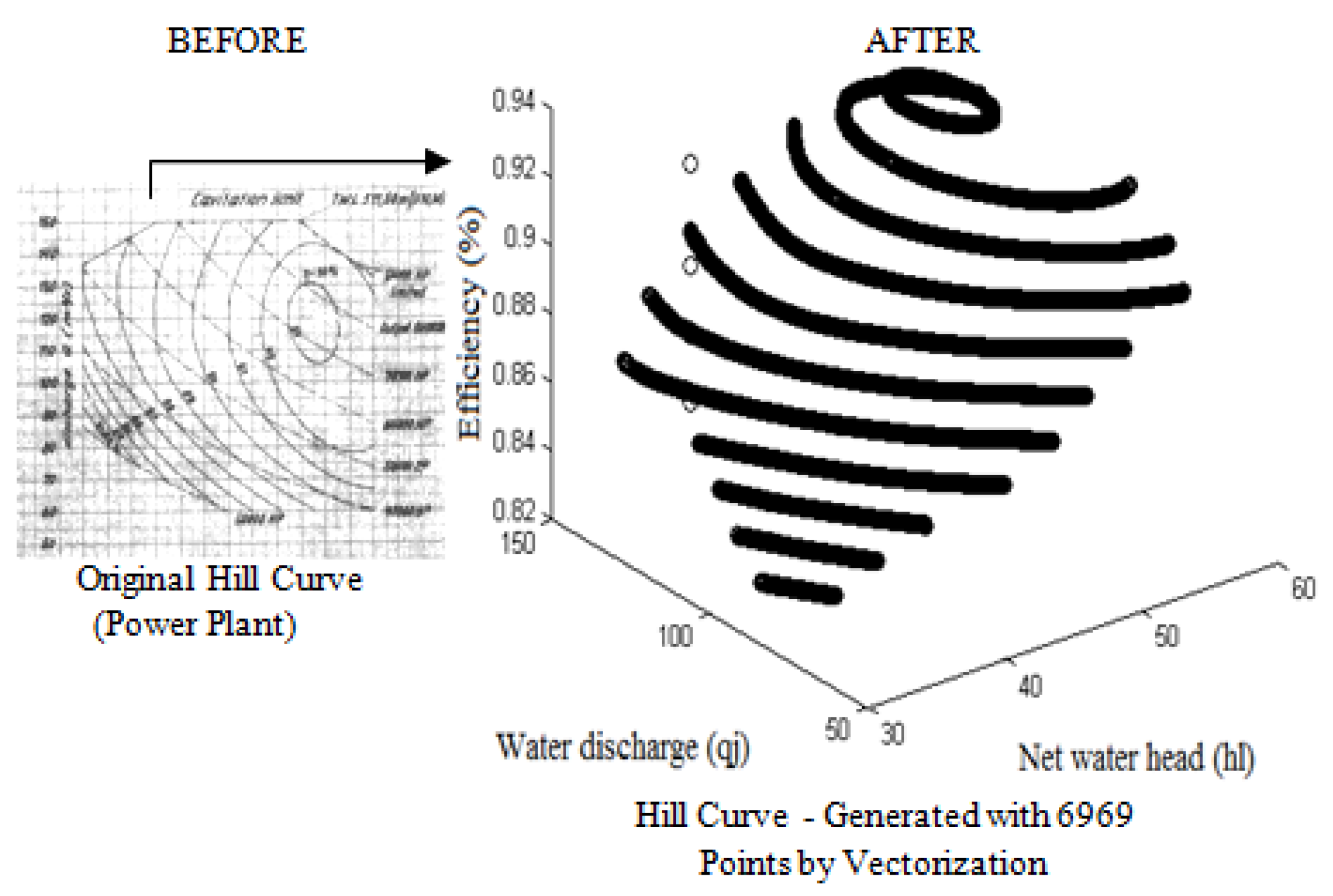
2.1.2. Adjustment of the Model from Data

Although different efficiency models in the literature exist, in this work the productivity modeling is described by the quadratic function shown in Equation (8),

$$\begin{array}{c}\hfill {\eta }_{jt}={\rho }_{0j}+{\rho }_{1j}h{l}_{jt}+{\rho }_{2j}{q}_{jt}+{\rho }_{3j}h{l}_{jt}{q}_{jt}+{\rho }_{4j}h{l}_{jt}^2+{\rho }_{5j}{q}_{jt}^2,\end{array}$$

(8)

where ${\eta }_{jt}$ is the productivity (in %) of each turbine-generator $\left(j\right)$ at interval $\left(t\right)$. The terms ${\rho }_{0j},\dots ,{\rho }_{5j}$ are the production coefficients generated using information about the Hill Curve. The term $h{l}_{jt}$ is the net water head (in m) of each turbine generator $\left(j\right)$ at time $\left(t\right)$ and $q_{jt}$ is the water discharge (in each turbine-generator $\left(j\right)$ at interval $\left(t\right)$.

This work addresses a real study in an HPP installed in Brazil where the plant has a single Hill Curve. The power production ($p{h}_{jt}$) defines the unit’s global efficiency by the product of the efficiencies of generators and turbines. Even though the generator’s efficiency can be considered constant over a wide range of operations, the turbine efficiency is dependent on the net head ($h{l}_{jt}$) and the turbine water discharge ($q_{jt}$). The relationship between these variables is relatively complex and typically described by a curve known as the Hill Curve [11]. Keeping in mind that the Hill Curve contains the information of water discharge, net head, and power generated, we performed a non-linear multi-variable regression process to obtain the operational coefficients from the original Hill Curve data depicted in Figure 1—left side. This strategy is considered a machine learning approach in which it was possible to learn from data.

A pre-processing was performed from the Hill Curve. The image went through a vectorization process, and thus we generated a 6969 point dataset ($q_{jt}$, $h{l}_{jt}$, ${\eta }_{jt}$). For the regression, the water discharged ($q_{jt}$) boundaries adopted were [70, 140] (m${}^3$/s) and the net water head ($h{l}_{jt}$) boundaries [32, 56] (m). These two parameters were considered the regression independent variables. On the other hand, the dependent variable used was the productivity (${\eta }_{jt}$) with boundaries [83, 94] (%). Figure 1 shows the process described.

In the adopted regression process a randomized sub-sample (996 points) of the created dataset by vectorization method was used with Equation (8). The internal MATLAB statistic algorithms of Levenberg-Marquardt [31,32] were used in the regression process. With an adjusted R-Squared of 99%, general root-mean-square error (RMSE) equal to 0.00263 and a general p-Value < 0.0001, the estimated coefficients obtained are shown in

Table 1. Operating Coefficients—Estimation by Nonlinear Regression.

Coefficient	Estimation	RMSE	p-Value
${\rho }_{0j}$	0.1463	$5.74\times {10}^{-3}$	<0.0001
${\rho }_{1j}$	0.018076	$2.01\times {10}^{-4}$	<0.0001
${\rho }_{2j}$	0.0050502	$4.75\times {10}^{-5}$	<0.0001
${\rho }_{3j}$	−3.5254e-05	$5.69\times {10}^{-7}$	<0.0001
${\rho }_{4j}$	−0.00112337	$2.07\times {10}^{-6}$	<0.0001
${\rho }_{5j}$	−1.4507e-05	$1.67\times {10}^{-7}$	<0.0001

. These values obtained show that the results are significant.

Figure 2 shows the original (vectorized points—in black) data overlapping the calculation by regression process (applying Equation (8) with coefficients from Table 1 and the 6969 data points of ($q_{jt}$) and ($h{l}_{jt}$)—in red). The graph shows that the approach realized is satisfactory, giving credibility to the coefficients estimated by regression addressed here.

As the equations for calculating ${\eta }_{jt}$ depend directly on the $q_{jt}$ and $h{l}_{jt}$, the production function has been simplified and proposed here. The coefficients ${\rho }_{0j},\cdots ,{\rho }_{6j}$ generated in our approach are characteristic parameters of Brazilian HPP. In our modeling Equation (9) calculates the power production,

$$\begin{array}{c}\hfill p{h}_{jt}=G·[{\rho }_{0j}+{\rho }_{1j}h{l}_{jt}+{\rho }_{2j}{q}_{jt}+{\rho }_{3j}h{l}_{jt}{q}_{jt}+\end{array}$$

(9)

$${\rho }_{4j}h{l}_{jt}^2+{\rho }_{5j}{q}_{jt}^2]·[H{b}_{jt}-{\Delta }_{Hjt}]·q_{jt},$$

where the $p{h}_{jt}$ is electric power for each turbine-generator (j) at interval (t). G is gravity $(9.8·{10}^{-3}$ kg/m${}^2$ s${}^2)$. The terms ${\rho }_{0j}$, …, ${\rho }_{5j}$ are the productivity coefficients. The term $h{l}_{jt}$ is the net water head of each turbine-generator (j) at the interval (t). The $q_{jt}$ addresses the water discharge of each turbine-generator (j) at an interval (t). The ${\Delta }_{Hjt}$ means the losses of pipelines for each turbine-generator (j) at an interval (t) and the reservoir head is given by ($Hb$) for each turbine-generator (j) at an interval (t). Figure 3 shows the interpolated graphical representation of Equation (9), using the operating coefficients given in Table 1.

As the only available data regarding the HPP under study were provided by means of a Hill Curve, no hydro constraints, such as hydrological alterations caused by power generation on HPPs [33], could be considered.

2.1.3. Optimization Modelling

The following model for maximizing hydroelectric productivity is then considered. Let the decision variable transposed vector be denoted by

$$x=[q_{1t},q_{2t},\dots ,q_{jt}],$$

in which each decision variable $q_{jt}\in \mathbb{R}$ is bounded by the lower and upper limits of the water discharge ($q_{jt}^{min}$ and $q_{jt}^{max}$, respectively), for each turbine-generator. The composed objective function is presented by Equation (10)

$$MaximizeF\left(x\right)=\frac{{\sum }_{j=1}^{J\left(r\right)}p{h}_{jt}}{{\sum }_{j=1}^{J\left(r\right)}{q}_{jt}},$$

(10)

The adopted objective function, $F\left(x\right)$, is the ratio between the total power generated (${\sum }_{j=1}^{J\left(r\right)}p{h}_{jt}$) and the total water (${\sum }_{j=1}^{J\left(r\right)}{q}_{jt}$) used to perform the electric dispatch. Keep in mind that the smaller the amount of water needed to meet the generation demand, the higher the productivity will be. This objective function is subject to the following constraints:

• The power demand produced ((${\sum }_{j=1}^{J\left(r\right)}p{h}_{jt}$)) can be considered approximately equal to the power demand requested (D), with an acceptable error ($\epsilon =0.15\%MW$).

  $$D(1-\epsilon )\le \sum _{j=1}^{J\left(r\right)}p{h}_{jt}\le D(1+\epsilon ),$$
• The water discharge boundaries for each turbine-generator ($q_{jt}^{min}$ and $q_{jt}^{max}$ ).

  $$q_{jt}^{min}\le q_{jt}\le q_{jt}^{max},$$
• The electric power boundaries ($p{h}_{jk}^{min}$ and $p{h}_{jk}^{max}$) for each turbine-generator in operating zones ($Z_{jk}$).

  $$p{h}_{jk}^{min}\sum _{k=1}^{{\varnothing }_j}{Z}_{jk}\le p{h}_{jt}\le p{h}_{jk}^{max}\sum _{k=1}^{{\varnothing }_j}{Z}_{jk},$$
• Each turbine-generator has only one operating zone: on or off ($Z_{jk}$, on (1) or off (0)).

  $$Z_{jk}\in \{0,1\},\sum _{k=1}^{{\varnothing }_j}{Z}_{jk}\le 1.$$

To satisfy these four constraints, we consider a penalty factor in the objective function, so the final fitness function can be expressed as

$$\begin{array}{c}\hfill f^{\prime }=p\sum _i^{n}max{[0,p{h}_{jt}/q_{jt}]}^2.\end{array}$$

(11)

2.2. Evolutionary Meta-Heuristic Proposed: The Coral Reefs Optimization Algorithm

The Coral Reefs Optimization algorithm (CRO) is a type of evolutionary technique proposed in [34,35] that has been successfully applied in several optimization problems [36,37,38,39,40,41,42]. The CRO uses a $n\times m$ grid $\mathcal{R}$ (i.e., the coral reef), where each square (denoted by its coordinates (i,j)) can host a candidate solution to the problem $\mathbf{x}$ (i.e., a coral). The CRO’s framework can be summarized as follows:

(1)

Initialization. The algorithm is initialized by assigning random candidate solutions to a random number of squares of the grid, leaving the rest empty. Each solution is labeled with the problem’s objective function $f\left(\mathbf{x}\right)$ (i.e. the healthy function).

(2)

Reef formation. It is an iterative process that takes place over $\kappa$ iterations. At each iteration several operators or search procedures are applied to emulate the corals’ reproduction in the reef. Therefore, new candidate solutions are obtained and try to settle on the reef. If the square of the reef found (i,j) is free, the coral settles in the hole. If the square is occupied, the candidate solution fights with the settled solution and the one with higher health function stays in the hole. If the new candidate cannot settle, it tries to find a new square, but after $\lambda$ attempts without finding a place to grow, the candidate solution is discarded.

(3)

Predation. Once settlement of new corals has taken place, a predation phase may occur with probability $P_{\psi }$. Should predation happen, a percentage of the reef has preyed and solutions previously settled are lost. Thus leaving holes for new candidate solutions (with bad health functions) from other areas of the search space, to enter the reef (and escape from local minima).

(4)

Stop. if halting criteria are satisfied; otherwise go to step (2) for the next cycle.

The best individual in the reef is considered to be the final solution to the problem.

The CRO algorithm can implement different search procedures during the reef’s formation to obtain new candidate solutions (it is an algorithm defined in exploitation, not in exploration). In this paper the operators selected as search procedures in the CRO are the following:

• Harmony Search mutation (HS): Mutation is recreating the Harmony Search algorithm [43]. New candidate is obtained: using the same values of the component from other reefs’ coral, with a probability HMCR$\in [0,1]$ (Harmony Memory Considering Rate); or performing slight modifications to the candidate, with a probability PAR (Pitch Adjusting Rate) $\in [0,1]$;
• Differential Evolution mutation (DE): Mutation implementing a Differential Evolution algorithm [44]. New candidates are obtained by combining a reef’s coral $\mathbf{x}$ with a perturbation vector ${\mathbf{x}}^{\prime }$. Two different strategies have been used to find the perturbation:
  DEB: $x_i^{\prime }=x_i^{best}+F(x_i^2-x_i^3)$ (using the best), and
  DER: $x_i^{\prime }=x_i^1+F(x_i^2-x_i^3)$ (on a random basis)
  (where F stands for the evolution factor that weights the perturbation amplitude, in our case $F=0.1$);
• Differential Evolution mutation with crossover (DEX): Mutation recreating the Differential Evolution algorithm [44]. New candidates are obtained after a crossover is applied between a coral from the reef $\mathbf{x}$ and a perturbation vector ${\mathbf{x}}^{\prime }$ generated by DER.
• Gaussian mutation (GM): The new candidate is obtained by applying gaussian mutation to a coral from the reef ($x_i^{\prime }=x_i+\delta N_i(0,1)$, where $N_i(0,1)$) is a random number following the Gaussian distribution. The Gaussian probability density function is:

  $$f_{G(0,{\sigma }^2)}\left(x\right)=\frac{1}{\sigma \sqrt{2\pi }}{e}^{-\frac{x^2}{2{\sigma }^2}}.$$

  where $\sigma$ value linearly decreases during the run, from $0.2·(A-B)$ to $0.02·(A-B)$, being $[B,A]$ the search domain. Therefore, at the beginning the mutation is strong while at the end it is a fine tuning.

On the other hand, the Coral Reefs Optimization with Substrate Layer algorithm (CRO-SL) [29,45] is a multi-method ensemble based on in the standard CRO algorithm, yet with a structure that promotes competitive co-evolution using the layers deployed. Each layer proposed implements a different search strategy, operator, constraint, repairing function, etc., although the use of diverse search operators is the most common mechanism for the CRO-SL. In this paper, each layer implements an exploration operator, and the procedures used are the same as those described for the classic CRO. In Section 3, the nomenclature used to refer to these layers is as follows: (1) $CR{O}_{\left(1\right)}$ for a layer implementing Harmony Search mutation, (2) $CR{O}_{\left(2r\right)}$ for a layer using Differential Evolution mutation, (3) $CR{O}_{\left(3r\right)}$ for a layer implementing Differential Evolution mutation with crossover (DEX), and (4) $CR{O}_{\left(4\right)}$ for a layer using Gaussian mutation (GM). Figure 4 illustrates the experimental design of the CRO algorithm.

3. Experiments and Results

This section describes the specific aspects of the HPP studied and the design of experiments realized to find good solutions for the UC problem by applying different versions of the CRO algorithm. We considered data from a real hydroelectric plant installed in São Francisco river, Minas Gerais state, Brazil. At the request of the plant manager, mathematical modeling did not address the Unit Minimum up/Minimum down time constraint, as the HPP must keep all its turbine-generators on. Difficulty to obtain data from an HPP regarding the power production lead us to calculate them from the Hill Curve of an HPP (see Section 2.1.2).

3.1. Case Study and Parameter Settings

The HPP considered in this paper has a capacity to produce 396MW/h, operating with six turbine-generators. The HPP presents constraints such as water discharge ($q_{jt}$), water discharge boundaries per turbine-generator ($q_{jt}^{min}$ and $q_{jt}^{max}$), and electricity produced per generator ($p{h}_{jt}$). According to these constraints, $q_{jt}$ must be in the range $[70,140]$ m${}^3$/s and $p{h}_{jt}$ must be in the range $[35,66]$ MW. In the simulation reported in this work all the power units were considered to be turned on to produce energy. The optimization algorithms need to receive system inputs of reservoir head ($H_b$) value, which is the fall height (in m) of the reservoir, in the range $[32,56]$.

The conducted experiments show the proposed modeling considering two stages: (1) the first step was to test all algorithms performing the daily electric dispatch. The CRO versions were compared in this case against two standard optimizers; and (2) the second step verifies the results obtained by the algorithms in hourly electric dispatches.

The results in both cases show the best solution archived in the last generation of all algorithms. After experimentation, inference methodology was conducted to investigate if the differences between the tested algorithms exist or not, when tackling the generation scheduling problem in this real HPP. We performed the computational simulation using an Intel CoreTM i7 with [email protected] GHz and 16 GB RAM, with Windows 10 operating system.

To verify the performance of the results of the CRO algorithm versions applied in this work, a real encoding Genetic algorithm (RGA) [46] and a Differential Evolution (DE) approach [44] have been chosen to compare results. We chose these approaches since RGA and DE have obtained good results in solving the UC problem in previous works. The initialization parameters used for all algorithms were: population size equal to 120, and the total number of generations equal to 120. Specifically for AG, a crossover rate equal to 0.6 and a mutation equal to 0.5 were used, in which this operator performed the polynomial mutation. In DE algorithms, $F=0.1$ and $CR=0.5$ are used in both strategies: DE(best/1/bin) and DE(rand/1/bin). The CRO algorithm used as a probability of death a value equal to 0.1, the number of jumps is equal to 3, and the number of depleted corals is equal to 10% of the population. All parameters were defined empirically. Each algorithm was performed 30 times to conduct the statistical analysis of the results. Figure 5 exemplifies the simulation strategy adopted.

3.2. Daily Dispatch Programming Experiment

This experiment conducts the daily operation for electric dispatch. The idea is to verify if the algorithms find feasible solutions respecting the constraints. In our experiment, the daily schedule used was totally random. Results obtained by each algorithm for five main characteristics: water discharged, net water head, losses, efficiency, and power produced (the terms in Equation (9) were used to construct response surface graphs via data interpolation. In general, the amount dispatched by each generator cannot be drastically changed, as it is not possible to decrease the speed of the generator to achieve this and dramatic changes can damage the dam. The value adopted as an input system in relation to the hydraulic head of the reservoir ($Hb$) was 55 $\left(m\right)$, which means that the reservoir has a higher level of capacity production. As it can be seen in response surfaces presented in this section, in general, all the algorithms tested respect the limits of power and water discharge rates, because the values found are between the range established by power and water discharge constraints. The solutions found by the stochastic algorithms used in this work report that it is possible to realize the operation using distinct dispatches per turbine-generator.

The graphics represent the values obtained for optimized water discharge in each hour, as well as the values of net water head, penstock losses, efficiency, and power generated. The small variations prove that the algorithms found solutions that do not drastically alter the unit dispatch (turbine-generators). This fact is very important in terms of the HPP generation and, indirectly, this dynamic minimizes the cost of maintaining these machines. Therefore, an ideal pattern for graphics is seen when there is little discrepancy on the response surface. We discuss here the behavior of some algorithms tested in this work. Among the mutation strategies used in the CRO algorithm, when using Gaussian mutation ($CR{O}_{\left(4\right)}$), showed in Figure 6, we can notice that the response surface constructed from the daily generation data has the least shape change.

This indicates that the optimized flow rates are different per generating unit, but it does not change very abruptly with the change in demand every hour. In addition, it reached the highest efficiency levels of each turbine-generator units among the tested algorithms. The same behavior is observed when checking the response surface presented by the DE/best/1/bin (DEB) and DE/rand/1/bin (DER) algorithms, showed by Figure 7 and Figure 8. The detail observed in the results of DEB and DER are similar to solutions archived by $CR{O}_{\left(4\right)}$, with some sharp disturbances.

The Real Genetic Algorithm (RGA—Figure 9) shows a sudden change in generation every hour. The behavior of turbine-generators modifying the power generated, as well as the CRO with Harmony mutation ($CR{O}_{\left(1\right)}$—Figure 10) and CRO uses mutation based on the DE strategies ($CR{O}_{\left(2b\right)}$ and $CR{O}_{\left(2r\right)}$—Figure 11 and Figure 12). When using the DE with crossover, ($CR{O}_{\left(3r\right)}$), we notice that the result is more stable than when using the two point crossover operation as well, as can be seen in Figure 13.

After verifying the behavior of each mutation applied to the CRO separately, we have shown that the CRO with a Gaussian mutation obtains the best results among all algorithms tested. Thus, the CRO algorithm was applied to solve the problem using substrates (CRO-SL) in order to verify the influence of the Gaussian mutation in combination with other search operators. As we can see, the Gaussian mutation improves the results of Harmony (Figure 14—($CR{O}_{(1,4)}$), both DE mutations implemented (Figure 15 and Figure 16—($CR{O}_{(2b,4)}$) and ($CR{O}_{(2r,4)}$), respectively), and the DE with crossover ($CR{O}_{(3r,4)}$), which can be seen in Figure 17.

To check out the algorithm’s performance in terms of demand requested and total water discharged, Figure 18 shows the results obtained with the different algorithms considered. It is possible to see that the generated power demand of all meta-heuristics was achieved respecting the constraints. Besides this, it is possible to see that all algorithms respected the water discharge limits saving resources to perform the operation when compared to the “usual mode of operation” system.

Table 2. Water saved in daily (d) power production. Million liters (mi). In bold the best results found.

D	RGA	DEB	DER	${\mathit{CRO}}_{\left(1\right)}$	${\mathit{CRO}}_{\left(2\mathit{b}\right)}$	${\mathit{CRO}}_{\left(2\mathit{r}\right)}$
255	0.40	0.71	0.70	−0.36	1.19	0.79
265	1.20	1.68	1.75	−0.25	0.93	1.87
275	2.49	2.66	2.49	4.91	3.61	2.76
285	2.98	3.46	3.43	2.01	3.11	3.59
295	2.14	4.12	3.88	4.78	4.32	4.30
305	3.43	4.62	4.25	3.52	5.53	4.68
315	2.95	4.93	4.78	3.06	4.85	5.07
325	3.03	4.57	4.76	3.66	6.23	5.22
335	3.50	4.54	4.03	2.01	4.49	5.02
345	3.09	4.35	4.51	3.50	3.27	4.63
355	3.27	3.72	3.73	8.36	2.78	3.88
365	1.17	2.64	2.49	3.20	2.33	2.87
365	1.35	2.58	2.69	3.20	3.06	2.87
355	3.37	3.19	3.78	8.36	3.74	3.91
345	4.10	4.47	4.52	3.50	4.32	4.63
335	4.46	4.81	5.11	2.01	4.81	5.06
325	3.59	5.04	5.02	3.66	6.21	5.19
315	3.17	4.45	4.97	3.06	5.71	5.09
305	3.66	4.62	4.56	3.52	5.29	4.75
295	2.67	4.06	4.18	4.78	4.27	4.22
285	2.99	3.46	3.46	2.29	3.59	3.58
275	2.33	2.66	2.58	4.91	3.60	2.82
265	1.37	1.74	1.82	2.10	1.22	1.85
255	0.61	0.71	0.70	−0.36	1.48	0.84
ASW (m${}^{\mathbf{3}}$/s)	63.3	83.8	84.2	79.4	89.9	89.5
ASW (L/day)	227.9 mi	301.7 mi	303.1 mi	285.9 mi	323.8 mi	322.2 mi
D	${\mathit{CRO}}_{\left(\mathbf{3}\mathit{r}\right)}$	${\mathit{CRO}}_{\left(\mathbf{4}\right)}$	${\mathit{CRO}}_{(\mathbf{1},\mathbf{4})}$	${\mathit{CRO}}_{(\mathbf{2}\mathit{b},\mathbf{4})}$	${\mathit{CRO}}_{(\mathbf{2}\mathit{r},\mathbf{4})}$	${\mathit{CRO}}_{(\mathbf{3}\mathit{r},\mathbf{4})}$
255	0.85	1.59	0.69	1.42	1.68	0.71
265	1.73	2.83	1.88	2.80	2.69	1.72
275	2.71	3.76	2.70	3.52	3.69	2.83
285	3.06	4.65	3.37	4.55	4.55	3.47
295	4.23	5.33	4.16	5.10	5.30	4.26
305	4.05	5.94	4.55	5.06	5.75	4.79
315	5.04	6.37	4.80	6.08	5.96	4.90
325	4.90	6.39	5.15	5.06	5.93	4.89
335	5.02	6.24	4.85	6.12	5.95	4.78
345	4.57	5.78	4.62	5.63	4.89	4.62
355	3.73	5.33	3.70	4.92	2.50	4.04
365	2.71	4.10	2.88	3.94	3.74	2.84
365	2.95	4.12	2.88	4.18	3.99	2.83
355	3.86	5.13	3.70	5.14	3.63	5.88
345	4.59	6.10	4.60	5.82	5.30	4.59
335	5.02	6.32	5.03	6.22	6.27	5.12
325	5.25	6.52	5.37	5.86	6.28	5.13
315	5.14	6.21	5.10	6.09	6.19	5.31
305	4.49	5.94	4.55	5.44	5.83	4.85
295	4.25	5.33	4.35	5.29	5.34	4.37
285	3.54	4.70	3.57	4.64	4.62	3.68
275	2.82	3.69	2.70	3.62	3.75	2.64
265	1.66	2.83	1.88	2.80	2.74	1.86
255	0.79	1.74	0.69	1.80	1.71	0.71
ASW (m${}^{\mathbf{3}}$/s)	87.0	116.9	87.8	111.1	108.3	90.8
ASW (L/day)	313.2 mi	420.9 mi	315.9 mi	399.9 mi	389.8 mi	326.9 mi

shows the results of water (in m${}^3$/s) projection savings in energy production. It is possible to verify that for all demands considered, the meta-heuristics save important amounts of water. If we focus on the details of the best proposed approaches, we can see that $CR{O}_{\left(4\right)}$ delivered the demand requested per hour; it used a much lower volume of water than the other approaches in the energy production process. Please note that the $CR{O}_{\left(4\right)}$ strategy was able to save 116.92 m${}^3$/s over the course of the day. In a projection, this saving is equivalent to 420 million(mi) liters of water per day. Analyzing the table we can also see that, using the sub-layer approach, Gaussian Mutation contributed to an improvement in results when combined with the other mutation strategies used in this work. Especially when used with the DE(2b) mutation option followed by DE(2r), Harmony and DE(3r) saving respectively more: 76.1 mi, 67.6 mi, 30 mi and 13.7 mi litters of water per day as shown in Table 2.

3.3. Hourly Dispatch Programming Experiment

The simulation objective in hourly dispatch is to find the possible differences between the algorithms. To verify this behavior, for each meta-heuristic applied in this work, a demand of 325MW/h was established. This choice is based on the results presented in Table 2, in which 325MW/h achieved the greatest savings.

4. Discussion

This section will address a comparative discussion of the performance of meta-heuristics applied to solve the UC problem. Each algorithm was run 30 times to verify normality. To satisfy an effective test of the obtained solution samples, this work applied statistical inference to check the normality of samples and use some statistical tests that could reflect the mean differences of the applied algorithms. To test the normality of samples (N = 30) we used the Kolmogorov-Smirnov test (see [47]). We adopted $\alpha =0.05$ in all cases. Figure 19 shows the test results in which the algorithms CRO(4) and DE(best/1/bin) indicated that the behaviour of the sample is non-normal. This data proves that Kolmogorov-Smirnov with a p-Value metric results was bigger than 0.05 in these two cases. The other algorithms have a normal distribution according to the empirical distribution function (CDF) presented in Kolmogorov-Smirnov results. A non-parametric inference methodology was adopted to investigate the presence of differences (or not) in averages of algorithms solutions.

Figure 20 shows scatter and boxplot graphics for the 30 runs obtained for each algorithm. The scatter helps us understand the outliers that were identified in the boxplot chart on the RGA, $CR{O}_{\left(1\right)}$, $CR{O}_{\left(2b\right)}$ and $CR{O}_{\left(3r\right)}$. Boxplot is a descriptive and non-parametric statistical test which depicts the 25th percentile, 50th percentile (median), 75th percentile, and min and max values, and outliers (if present). Although some boxplots may show the location of the mean in relation to the median and quartiles, boxplots do not provide information about the true difference among means. However, since an overlap of the boxes can be seen for fitness values of algorithms tested, a statistical test needs to be performed in order to identify whether there is a difference among the algorithms. Keeping this point in mind and observing Figure 20, it is possible to argue that:

• visually we can see differences among the true means of $CR{O}_{\left(4\right)}$ and the rest of the algorithms, favouring $CR{O}_{\left(4\right)}$ version, but cannot perceive the overlap with others;
• it is not possible to conclude if a statistical significant difference of the means computed of RGA, $CR{O}_{\left(1\right)}$, $CR{O}_{\left(2b\right)}$, $CR{O}_{\left(2r\right)}$, and $CR{O}_{\left(3r\right)}$ algorithms exists (or not).

CRO-SL version is an ensemble approach, which works with sub-layers working as searching operators. Because of that, after observing the good result from the CRO with Gaussian mutation (the $CR{O}_{\left(4\right)}$ strategy), we investigated the influence of this mutation together with the other exploration mechanisms considered. Figure 21 shows the results combining a Gaussian mutation with Harmony and DE strategies.

We can see that the Gaussian mutation improves the results of CRO in the CRO-SL approach. If we consider the CRO-SL including a combination of Gaussian and Harmony substrates ($CR{O}_{(1,4)}$), the boxplot presents a lower dispersion of results, as well as the combinations made with the DE strategies, when comparing the results presented in the versions shown in Figure 20. According to our previous analysis, a statistical test needs to be performed in order to identify whether there is a difference among the algorithms. A Kruskal-Wallis [48] test and a non-parametric Tukey-type test [49] were used to test for differences among the mean ranks of the nine treatments/algorithms. Kruskal-Wallis results show with a p-Value of $2.04\times {10}^{-52}$ that there exists a statistically significant difference, with $\alpha =5\%$, between the algorithms results. The Kruskal-Wallis test tells us if the obtained results are significantly statistical, but does not indicate where differences are in the groups tested. The Tukey test [49] can be carried out to check if groups shows differences. The test conducts a full pairwise comparison, as shown in Figure 22. Figure 22 shows the result of the Tukey test confirming that $CR{O}_{\left(4\right)}$ configurations generate solutions with a higher fitness function values. However, we cannot say if there is a clear distinction between the $CR{O}_{(2b,4)}$ and $CR{O}_{(1,4)}$ solutions. Figure 23 shows plots of typical fitness evolution for each CRO-SL approach. It is possible to see the algorithm’s convergence in 120 generations. We can analyze the graphs and assert that the algorithms stabilized the average convergence starting with the 48th, 55th and 100th generations, to a fitness value equal to 0.50158 ($CR{O}_{\left(4\right)}$), 0.50148 ($CR{O}_{(1,4)}$) and 0.50152 ($CR{O}_{(2b,4)}$), respectively.

Table 3. General simulation report of 325 MW/h. The results in bold mean the maximum efficiency achieved.

${\mathit{CRO}}_{(1,4)}$|$\left(\mathit{Hb}\right)=55\mathit{m}$
UN	${\mathit{ph}}_{\mathit{jt}}$($\mathit{MW}$)	${\mathit{q}}_{\mathit{jt}}$(m${}^{\mathbf{3}}$/s)	${\mathit{\eta }}_{\mathit{jt}}$(%)	${\mathit{hl}}_{\mathit{jt}}$($\mathit{m}$)	${\mathbf{\Delta }}_{\mathit{Hjt}}$($\mathbf{m}$)
1	54.6	109.00	0.93	54.76	0.24
2	55.7	111.00	0.93	54.81	0.19
3	54.5	108.73	0.93	54.81	0.19
4	53.2	106.01	0.93	54.82	0.18
5	53.7	107.02	0.93	54.81	0.19
6	53.3	106.3	0.93	54.80	0.20
SUM	324.99	648.05	Flow in SCM: 653.1 (m${}^3$/s)
SUB	−0.01	5.05	Productivity index: 0.50148
${\mathit{CRO}}_{(\mathbf{2}\mathit{b},\mathbf{4})}$|$\left(\mathit{Hb}\right)=\mathbf{55}\mathit{m}$
UN	${\mathit{ph}}_{\mathit{jt}}$($\mathit{MW}$)	${\mathit{q}}_{\mathit{jt}}$(m${}^{\mathbf{3}}$/s)	${\mathit{\eta }}_{\mathit{jt}}$(%)	${\mathit{hl}}_{\mathit{jt}}$($\mathit{m}$)	${\mathbf{\Delta }}_{\mathit{Hjt}}$($\mathbf{m}$)
1	54.6	109.00	0.93	54.76	0.24
2	54.2	108.00	0.93	54.8	0.20
3	53.9	107.42	0.93	54.81	0.19
4	53	105.63	0.93	54.82	0.18
5	54.2	108.06	0.93	54.84	0.18
6	53.1	109.92	0.93	54.84	0.18
SUM	325.01	648.04	Flow in SCM: 653.1 (m${}^3$/s)
SUB	+0.01	5.15	Productivity index: 0.50152
${\mathit{CRO}}_{\left(\mathbf{4}\right)}$|$\left(\mathit{Hb}\right)=\mathbf{55}\mathit{m}$
UN	${\mathit{ph}}_{\mathit{jt}}$($\mathit{MW}$)	${\mathit{q}}_{\mathit{jt}}$(m${}^{\mathbf{3}}$/s)	${\mathit{\eta }}_{\mathit{jt}}$(%)	${\mathit{hl}}_{\mathit{jt}}$($\mathit{m}$)	${\mathbf{\Delta }}_{\mathit{Hjt}}$($\mathbf{m}$)
1	53.6	107	0.93	54.77	0.23
2	54.7	109	0.93	54.8	0.20
3	54.3	108.2	0.93	54.81	0.19
4	53.9	107.4	0.93	54.81	0.19
5	53.7	107.4	0.93	54.82	0.18
6	54.7	109.02	0.93	54.81	0.19
SUM	324.92	647.78	Flow in SCM: 653.1 (m${}^3$/s)
SUB	−0.08	5.32	Productivity index: 0.50155

contains the dispatch report of the algorithms. The saving resources can be addressed as follows: $CR{O}_{(1,4)}$ generates an economy of 5.05 m${}^3$/s, $CR{O}_{(2b,4)}$ perform an economy of 5.15 m${}^3$/s and $CR{O}_{\left(4\right)}$ show the best results saving 5.32 m${}^3$/s. In a monthly projection, the savings achieved by the CRO versions reach an amount of 13.27 billion liters of water using $CR{O}_{(1,4)}$ approach, 13.53 billion liters of water using the solution of $CR{O}_{(2b,4)}$, and 13.98 billion liters of water using the solution by the $CR{O}_{\left(4\right)}$ strategy. To supply a city of 300.000 citizens, it is necessary to have, on average, 1.1 billion liters [50]. In a city with a population of 2.4 million residents, for example, in a simple analogy, 13.98 billion liters are enough to guarantee the water supply for almost 1.5 months approximately. Please note that all turbine-generators worked in the maximum level of efficiency.

Finally, we would like to state that the $CR{O}_{\left(4\right)}$ version performed the electric dispatch operation in HPP, achieving competitive solutions. In results addressed here the $CR{O}_{\left(4\right)}$ obtained the highest water savings in a projection when compared to the results of standard evolutionary algorithms compared in this work and present in [50,51].

5. Conclusions

In this paper, we have dealt with a specific version of the generation scheduling by unit commitment problem in hydro-power plants (HPPs). This work describes an efficient mathematical modeling for including hydraulic losses in penstocks at HPPs, allowing a more accurate calculation of the power production. This new formulation of the problem has been applied in an active generation scheduling problem in a real HPP in Brazil. A fresh meta-heuristic, the Coral Reefs Optimization algorithm (CRO) has been proposed for solving this problem, testing different variants of the algorithm, including a different exploration for the coral reef’s population. Upon the application of the model and the respective analysis of results, the contributions are:

• Proposal of an effective mathematical modeling to power electric dispatch in HPP. The proposed model extends the electric power equation (Equation (9)), bringing modularity to the obtaining of ${\eta }_{jt}$ (using regression fit) and $h{l}_{jt}$ (fluid mechanics’ model) terms. This modeling has been described and discussed in detail, being easily replicable.
• Inclusion of a hydraulic losses model in the mathematical modeling, to bring greater reality to the dynamics of the electric dispatch problem. In this sense, net water head ($h{l}_{jt}$) was obtained (Equation. (7)).
• Generation of a dataset, using regression techniques, featuring power plants’ Kaplan-type turbines. Operating Coefficients in Equation (8) were estimated using Nonlinear Regression and presented in Table 1.
• Proposal and testing of the CRO algorithm using a combination of search operators or search operators independently. In this work, the latter has concluded on best results when the CRO with Gaussian mutation was used, outperforming real encoded genetic algorithms and differential evolution.
• Proposal of a statistical inference methodology to compare results from the meta-heuristics has been applied. To test the samples’ normality, the Kolmogorov-Smirnov test was implemented, showing that the behaviour using CRO(4) and DE(best/1/bin) algorithms is non-normal. Also, Kruskal-Wallis test was used to determine the differences among the mean ranks, resulting in statistically significant difference between the algorithms results. Finally, Tukey test was performed, confirming that CRO(4) configurations generate solutions with higher fitness function values.

The experimental results obtained show that the proposed methods based on the CRO algorithm converged for satisfactory results. The best performing CRO approach was the CRO with Gaussian mutation, which showed a competitive performance, better than previous algorithms for this problem such as real coded genetic algorithms or Differential Evolution approaches. The CRO-SL also showed a good performance, but it was not possible to statistically confirm that CRO-SL outperforms the CRO with the Gaussian Mutation ($CR{O}_{\left(4\right)}$). In the daily dispatch experiment, the $CR{O}_{\left(4\right)}$ obtained the best results, followed by the CRO-SL with Gaussian Mutation and DE mutation $CR{O}_{(2r,4)}$ and by $CR{O}_{\left(3r\right)}$ CRO with DE with mutation/crossover. We also conducted an hourly power dispatch in which the CRO with Gaussian Mutation obtained again the best result, producing a solution able to save approximately 13.98 billion liters of water every month, in respect to the current HPP operating mode. Future works comprise the proposal of local search procedures to improve the performance of the CRO meta-heuristic. Also, research on new solving schemes to UC-related problems, in a cascade power production system, and the inclusion of hydro-logical alterations caused from power generation, will be pursued in the near future.

References

1. Padhy, N. Unit Commitment—A Bibliographical Survey. IEEE Trans. Power Syst. 2004, 19, 1196–1205. [Google Scholar] [CrossRef]
2. Yang, L.; Li, W.; Xu, Y.; Zhang, C.; Chen, S. Two novel locally ideal three-period unit commitment formulations in power systems. Appl. Energy 2020, 284, 1–19. [Google Scholar]
3. Arce, A.; Soares, S.; Ohishi, T.; Cicogna, A. Unit Commitment of Hydro Dominated Systems. Electr. Power Syst. Res. 2008, 9, 1–17. [Google Scholar]
4. Brito, B.; Finardi, E.; Takigawa, F. Unit-commitment via logarithmic aggregated convex combination in multi- unit hydro plants. Electr. Power Syst. Res. 2020, 81, 1–7. [Google Scholar]
5. Ceran, B.; Jurasz, J.; Wroblewski, R.; Guderski, A.; Ztotecka, D.; Kazmierczak, L. Impact of the Minimum Head on Low-Head Hydropower Plants Energy Production and Profitability. Energies 2020, 13, 6728. [Google Scholar] [CrossRef]
6. Abdi, H. Profit-based unit commitment problem: A review of models, methods, challenges, and future directions. Renew. Sustain. Energy Rev. 2020, 1, 1–28. [Google Scholar] [CrossRef]
7. Kong, J.; Skjelbred, H.; Fosso, O. An overview on formulations and optimization methods for the unit-based short-term hydro scheduling problem. Electr. Power Syst. Res. 2020, 118, 1–14. [Google Scholar] [CrossRef]
8. Daadaa, M.; Seguin, S.; Demeester, K.; Anjos, M. An optimization model to maximize energy generation in short-term hydropower unit commitment using efficiency points. Int. J. Electr. Power Energy Syst. 2021, 125, 1–8. [Google Scholar] [CrossRef]
9. Yoo, J.H. Maximization of hydropower generation throught the application of a linear programming model. J. Hydrol. 2013, 376, 182–187. [Google Scholar] [CrossRef]
10. Bento, P.; Mariano, S.; Calado, M.; Ferreira, L. A Novel Lagrangian Multiplier Update Algorithm for Short-Term Hydro-Thermal Coordination. Energies 2020, 13, 1–19. [Google Scholar]
11. Finardi, E.; da Silva, E.L. Unit commitment of single hydroelectric plant. Electr. Power Syst. Res. 2005, 75, 116–123. [Google Scholar] [CrossRef]
12. Zhang, R.; Zhow, J.; Ouyang, S.; Wang, X.; Zhang, H. Optimal operation of multi-reservoir system by multi-elite guide particle swarm optimization. Int. J. Electr. Power Energy Syst. 2013, 48, 58–68. [Google Scholar] [CrossRef]
13. Na, F.; Zhou, J.; Zhang, R.; Liu, Y.; Zhang, Y. A hybrid of real coded genetic algorithm and artificial fish swarm algorithm for short-term optimal hydrothermal scheduling. Int. J. Electr. Power Energy Syst. 2014, 62, 617–629. [Google Scholar]
14. Glotic, A.; Glotic, A.; Kitak, P.; Pihler, J.; Ticar, I. Parallel Self-Adaptive Differential Evolution Algorithm for Solving Short-Term Hydro Scheduling Problem. IEEE Trans. Power Syst. 2014, 29, 2347–2358. [Google Scholar] [CrossRef]
15. He, Z.; Zhou, J.; Jia, H.; Lu, C. Long-term joint scheduling of hydropower station group in the upper reaches of the Yangtze River using partition parameter adaptation differential evolution. Eng. Appl. Artif. Intell. 2020, 81, 1–13. [Google Scholar] [CrossRef]
16. Zhang, R.; Chen, D.; Yao, W.; Ba, D.; Ma, X. Non-linear fuzzy predictive control of hydroelectric system. IET Gener. Transm. Distrib. 2017, 11, 1966–1975. [Google Scholar] [CrossRef]
17. Yang, Y.; Wu, L. Machine learning approaches to the unit commitment problem: Current trends, emerging challenges, and new strategies. Electr. J. 2021, 34, 369–389. [Google Scholar]
18. Nan, Y.; Di, Y.; Zheng, Z.; Jiazhan, C.; Daojun, C.; Xiaoming, W. MResearch on modelling and solution of stochastic SCUC under AC power flow constraints. IET Gener. Transm. Distrib. 2018, 12, 3618–3625. [Google Scholar] [CrossRef]
19. Cioffi, F.; Gallerano, F. Multi-objective analysis of dam release flows in rivers downstream from hydropower reservoirs. Appl. Math. Model. 2013, 36, 2868–2889. [Google Scholar] [CrossRef] [Green Version]
20. Doganis, P.; Sarimveis, H. Optimization of power production through coordinated use of hydroelectric and conventional power units. Appl. Math. Model. 2014, 38, 2051–2062. [Google Scholar] [CrossRef]
21. Reddy, K.; Panwar, L.; Panigrahi, B.; Kumar, R. Binary whale optimization algorithm: A new metaheuristic approach for profit-based unit commitment problems in competitive electricity markets. Eng. Optim. 2019, 51, 369–389. [Google Scholar] [CrossRef]
22. Perumal, R.; Krishnan, m.; Subramanian, K. A hybrid LR-FA technique to optimize the profit function of gencos in a restructured power system. Electr. Power Syst. Res. 2012, 32, 113–120. [Google Scholar] [CrossRef]
23. Singh, A.; Khamparia, A. A hybrid whale optimization-differential evolution and genetic algorithm based approach to solve unit commitment scheduling problem: WODEGA. Sustain. Comput. Inform. Syst. 2020, 28, 1–10. [Google Scholar] [CrossRef]
24. Marcelino, C.; Baumann, M.; Carvalho, L.; Chibeles-Martins, N.; Weil, M.; Almeida, P.; Wanner, E. A combined optimisation and decision-making approach for battery-supported HMGS. J. Oper. Res. Soc. 2020, 71, 762–774. [Google Scholar] [CrossRef]
25. Marcelino, C.; Almeida, P.; Wanner, E.; Baumann, M.; Weil, M.; Cavalho, L.; Miranda, V. Solving security constrained optimal power flow problems: A hybrid evolutionary approach. Appl. Intell. 2018, 48, 3672–3690. [Google Scholar] [CrossRef] [Green Version]
26. Sharma, D.; Trivedi, D.; Srinivasan, D.; Thillainathan, L. Multi-agent modeling for solving profit based unit commitment problem. Appl. Soft Comput. 2013, 13, 3751–3761. [Google Scholar] [CrossRef]
27. Dhaliwal, J.; Dhillon, J. Profit based unit commitment using memetic binary differential evolution algorithm. Appl. Soft Comput. 2019, 81, 1–20. [Google Scholar] [CrossRef]
28. Salcedo-Sanz, S. A review on the coral reefs optimization algorithm: New development lines and current applications. Prog. Artif. Intell. 2017, 6, 1–15. [Google Scholar] [CrossRef]
29. Garcia-Hernandez, L.; Garcia-Hernandez, J.; Salas-Morena, L.; Carmona-Munoz, C.; Alghamdi, N.; Valente de Oliveira, J.; Salcedo-Sanz, S. Addressing Unequal Area Facility Layout Problems with the Coral Optimization algorithm with Substrate Layers. Eng. Appl. Artif. Intell. 2020, 93, 1–11. [Google Scholar] [CrossRef]
30. Massey, B. Mech. Fluids; Spon Press: Abingdon, VA, USA, 2012. [Google Scholar]
31. Levenberg, K. A Method for the Solution of Certain Non-Linear Problems in Least Squares. Q. Appl. Math. 1944, 2, 164–168. [Google Scholar] [CrossRef] [Green Version]
32. Marquardt, D. An Algorithm for Least-Squares Estimation of Nonlinear Parameters. SIAM J. Appl. Math. 1963, 11, 431–441. [Google Scholar] [CrossRef]
33. Braun-Cruz, C.; Tritico, H.; Beregula, R.; Girard, P.; Zeihofer, P.; Ribeiro, L.; Fantin-Cruz, I. Evaluation of Hydrological Alterations at the Sub-Daily Sacale Caused by a Small Hydroelectric Facility. Water 2021, 13, 206. [Google Scholar] [CrossRef]
34. Salcedo-Sanz, S.; Del Ser, J.; Landa-Torres, I.; Gil-Lopez, S.; Portilla-Figueras, J.A. The coral reefs optimization algorithm: A novel metaheuristic for efficiently solving optimization problems. Sci. World J. 2014, 2014, 1–15. [Google Scholar] [CrossRef] [PubMed]
35. Salcedo-Sanz, S.; Del Ser, J.; Landa-Torres, I.; Gil-Lopez, S.; Portilla-Figueras, J.A. The coral reefs optimization algorithm: An efficient meta-heuristic for solving hard optimization problems. In Proceedings of the 15th International Conference on Applied Stochastic Models and Data Analysis (ASMDA2013), Mataró (Barcelona), Spain, 25–28 June 2013; Volume 1, pp. 751–758. [Google Scholar]
36. Garcia-Hernandez, L.; Salas-Morera, L.; Carmona-Muñoz, C.; Abraham, A.; Salcedo-Sanz, S. A Hybrid Coral Reefs Optimization - Variable Neighborhood Search Approach for the Unequal Area Facility Layout Problem. IEEE Access 2020, 8, 134042–134050. [Google Scholar] [CrossRef]
37. García-Hernandez, L.; Salas-Morera, L.; Carmona-Muñoz, C.; Abraham, A.; Salcedo-Sanz, S. A novel multi-objective Interactive Coral Reefs Optimization algorithm for the Unequal Area Facility Layout Problem. Swarm Evol. Comput. 2020, 55, 100688. [Google Scholar] [CrossRef]
38. Camacho-Gómez, C.; Marsá-Maestre, I.; Giménez-Guzmán, J.; Salcedo-Sanz, S. A Coral Reefs Optimization algorithm with substrate layer for robust Wi-Fi channel assignment. Soft Comput. 2019, 23, 12621–12640. [Google Scholar] [CrossRef]
39. Durán-Rosal, A.; Gutiérrez, P.; Salcedo-Sanz, S.; Hervás-Martínez, C. A statistically-driven Coral Reef Optimization algorithm for optimal size reduction of time series. Appl. Soft Comput. 2018, 63, 139–153. [Google Scholar] [CrossRef]
40. Sánchez-Montero, R.; Camacho-Gómez, C.; López-Espí, P.; Salcedo-Sanz, S. Optimal Design of a Planar Textile Antenna for Industrial Scientific Medical (ISM) 2.4 GHz Wireless Body Area Networks (WBAN) with the CRO-SL Algorithm. Sensors 2018, 18, 1982. [Google Scholar] [CrossRef] [PubMed] [Green Version]
41. Salcedo-Sanz, S.; García-Díaz, P.; Del-Ser, J.; Bilbao, M.; Portilla-Figueras, J. A novel Grouping Coral Reefs Optimization algorithm for optimal mobile network deployment problems under electromagnetic pollution and capacity control criteria. Expert Syst. Appl. 2016, 55, 388–402. [Google Scholar] [CrossRef]
42. Salcedo-Sanz, S.; Camacho-Gómez, C.; Mallol-Poyato, R.; Jiménez-Fernández, S.; Del Ser, J. A novel Coral Reefs Optimization algorithm with substrate layers for optimal battery scheduling optimization in micro-grids. Soft Comput. 2016, 20, 4287–4300. [Google Scholar] [CrossRef]
43. Geem, Z.; Kim, J.; Loganathan, G. A new heuristic optimization algorithm: Harmony search. Simulation 2001, 76, 60–68. [Google Scholar] [CrossRef]
44. Storn, R.; Proce, K. Differential Evolution - A Simple and Efficient Heuristic for global Optimization over Continuous Spaces. J. Glob. Optim. 1997, 11, 341–359. [Google Scholar] [CrossRef]
45. Salcedo-Sanz, S.; Camacho-Gómez, C.; Molina, D.; Herrera, F. A coral reefs optimization algorithm with substrate layers and local search for large scale global optimization. In Proceedings of the IEEE Congress on Evolutionary Computation, CEC 2016, Vancouver, BC, Canada, 24–29 July 2016; pp. 3574–3581. [Google Scholar]
46. Deb, K.; Deb, D. Analysing mutation schemes for real-parameter genetic algorithms. Int. J. Artif. Intell. Soft Comput. 2014, 4, 1–28. [Google Scholar] [CrossRef]
47. Justel, A.; Pena, D.; Zamar, R. A multivariate Kolmogorov-Smirnov test of goodness of fit. Stat. Probab. Lett. 1997, 35, 251–258. [Google Scholar] [CrossRef] [Green Version]
48. Kruskal, W.; Wallis, W. Use of Ranks in One-Criterion Variance Analysis. J. Am. Stat. Assoc. 1952, 47, 583–621. [Google Scholar] [CrossRef]
49. Tukey, J. Comparing Individual Means in the Analysis of Variance. Biometrics 1949, 5, 99–114. [Google Scholar] [CrossRef] [PubMed]
50. Marcelino, C.; Carvalho, L.; Almeida, P.; Wanner, E.; Miranda, V. Application of Evolutionary Multiobjective Algorithms for solving the problem of Energy Dispatch in Hydroelectric Power Plants. Lect. Notes Comput. Sci. 2014, 4, 403–417. [Google Scholar]
51. Marcelino, C.; Wanner, E.; Almeida, P. A novel mathematical modeling approach to the electric dispatch problem: Case study using Differential Evolution algorithms. In Proceedings of the IEEE Congress on Evolutionary Computation (CEC), Cancun, Mexico, 20–23 June 2013; Volume 1, pp. 400–407. [Google Scholar]
Figure 1. Hill Curve - Vectorized points. Left: Hill Curve for a plant using Kaplan and installed in 1956. Each level of productivity (efficiency) in the range [83, 94] % was redesigned and, based on a vectorization algorithm, 6969 points were generated with the information regarding ( q j t ), ( h l j t ) and ( η j t ). Right: graph plot generated using the 6969 points obtained in the vectorization.
Energies 14 02443 g001
Figure 2. Hill Curve—Overlap: vectorized points of ( q j t ), ( h l j t ) and ( η j t ) and calculated points using ( q j t ), ( h l j t ) data, operative coefficients from regression (by Table 1) and Equation (8).
Energies 14 02443 g002
Figure 3. Hill Curve—Surface obtained: meshgrid created from [70, 140] ( q j t , in m 3 /s), [32,56] ( h l j t , in m), [83,93] ( η j t , in %) intervals using Equation (8).
Energies 14 02443 g003
Figure 4. (a) Reef’s setting process in CRO-SL. Each potential solution to the problem (larva) tries to settle down in any substrate, regardless of its origin substrate. (b) Example of layered reef and their different search strategies implemented (mutations and/or crossovers on each substrate).
Energies 14 02443 g004
Figure 5. Simulation strategy adopted. The (upper) part of the figure exemplifies the Daily dispatch programming experimentation. The (bottom) part of the figure exemplifies the Hourly dispatch programming experimentation.
Energies 14 02443 g005
Figure 6. CRO with Gaussian Mutation— C R O ( 4 ) . Results of Water discharge (m 3 /s). Net water head (m). Penstock (m). Efficiency (%) and Power generated (MW/h). Daily dispatch (24 h).
Energies 14 02443 g006
Figure 7. Differential Evolution (best/1/bin)—DEB. Results of Water discharge (m 3 /s). Net water head (m). Penstock (m). Efficiency (%) and Power generated (MW/h). Daily dispatch (24 h).
Energies 14 02443 g007
Figure 8. Differential Evolution (rand/1/bin)—DER. Results of Water discharge (m 3 /s). Net water head (m). Penstock (m). Efficiency (%) and Power generated (MW/h). Daily dispatch (24 h).
Energies 14 02443 g008
Figure 9. Real Genetic Algorithm—RGA. Results of Water discharge (m 3 /s). Net water head (m). Penstock (m). Efficiency (%) and Power generated (MW/h). Daily dispatch (24 h).
Energies 14 02443 g009
Figure 10. CRO with Harmony mutation— C R O ( 1 ) . Results of Water discharge (m 3 /s). Net water head (m). Penstock (m). Efficiency (%) and Power generated (MW/h). Daily dispatch (24 h).
Energies 14 02443 g010
Figure 11. CRO with DE Mutation (best/1/bin)— C R O ( 2 b ) . Results of Water discharge (m 3 /s). Net water head (m). Penstock (m). Efficiency (%) and Power generated (MW/h). Daily dispatch (24 h).
Energies 14 02443 g011
Figure 12. CRO with DE Mutation (rand/1/bin)— C R O ( 2 r ) . Results of Water discharge (m 3 /s). Net water head (m). Penstock (m). Efficiency (%) and Power generated (MW/h). Daily dispatch (24 h).
Energies 14 02443 g012
Figure 13. CRO with DE Mutation/Crossover (rand/1/bin)— C R O ( 3 r ) . Results of Water discharge (m 3 /s). Net water head (m). Penstock (m). Efficiency (%) and Power generated (MW/h). Daily dispatch (24 h).
Energies 14 02443 g013
Figure 14. CRO-SL with Harmony and Gaussian Mutations substrates— C R O ( 1 , 4 ) . Results of Water discharge (m 3 /s). Net water head (m). Penstock (m). Efficiency (%) and Power generated (MW/h). Daily dispatch (24 h).
Energies 14 02443 g014
Figure 15. CRO-SL with DE(best/1/bin) and Gaussian Mutation substrates— C R O ( 2 b , 4 ) . Results of Water discharge (m 3 /s). Net water head (m). Penstock (m). Efficiency (%) and Power generated (MW/h). Daily dispatch (24 h).
Energies 14 02443 g015
Figure 16. CRO-SL with DE(rand/1/bin) and Gaussian Mutation substrates— C R O ( 2 r , 4 ) . Results of Water discharge (m 3 /s). Net water head (m). Penstock (m). Efficiency (%) and Power generated (MW/h). Daily dispatch (24 h).
Energies 14 02443 g016
Figure 17. CRO-SL with (DEB/DER) and Gaussian Mutation substrates— C R O ( 3 r , 4 ) . Results of Water discharge (m 3 /s). Net water head (m). Penstock (m). Efficiency (%) and Power generated (MW/h). Daily dispatch (24 h).
Energies 14 02443 g017
Figure 18. Typical plot of power generated (MW/h)/water discharged (m 3 /s) through time in the Daily dispatch (24 h).
Energies 14 02443 g018
Figure 19. Empirical CDF of the meta-heuristics considered. Results obtained from 30 runs of each algorithm.
Energies 14 02443 g019
Figure 20. Scatter and Boxplot chart for the CRO with a single layer approach. Results obtained after 30 runs of the algorithm.
Energies 14 02443 g020
Figure 21. Scatter and Boxplot chart for the CRO-SL with Gaussian, Harmony and DE strategies. Results obtained after 30 runs of the algorithm.
Energies 14 02443 g021
Figure 22. Tukey test results obtained from 30 runs of the algorithm.
Energies 14 02443 g022
Figure 23. Best evolution’s obtained by CRO-SL algorithm with three different search strategies.
Energies 14 02443 g023