1. Introduction
Power converters have been a fundamental piece for the integration of renewable energies, which every day have a greater presence around the world [
1,
2,
3]. The boost converter is widely used to ensure the operation of electrical systems, such as photovoltaic systems [
4,
5], microgrids [
6,
7], and fuel cells [
8,
9,
10,
11]. For this, there are different topologies according to the needs of low or high power systems [
5,
12]. To ensure the desired output of the boost converter, control techniques of a pulse width modulated signal (PWM) are used. Different control techniques have been used to control the desired signals for the boost converter and other converters, such as the PI [
8,
13,
14,
15,
16], PID [
17,
18,
19], frequency-domain control techniques such as the method of sliding modes [
6,
20,
21], fuzzy logic [
22,
23], and inverse optimal control [
24,
25,
26].
The equations of state of power converters are sensitive to different disturbances, which is why many works focus on damping the effects of these separately with the methods mentioned above. To mention some of them, in [
17] they subject a boost converter to changes in the input variables and changes in the reference voltage separately, in [
6] the disturbance is a change in the voltage reference, with fixed parameters, in [
20] they subject a boost converter to variations in the load and changes in the sampling time of the control method, in [
14] they subject it to changes in the voltage reference, as well as in [
27], where they model different power conditioners under different initial conditions and different reference voltages, obtaining good results, using an adjustment similar to this work, however, the reference voltage changes are analyzed separately, not the subject to so many changes, nor is the extent of the adjustment analyzed. In [
28], through Lyapunov’s control theory, they subject the boost converter to disturbances in the load and input voltage. In [
25,
26], the inverse optimal control is implemented to a boost converter, while in [
26] it does not have any disturbance, and in [
25] the system is tested against a voltage drop of 3 volts.
The main problem is that solving the optimal control of nonlinear systems is extremely difficult because it must be solved by Hamilton-Jacobi-Bellman (HJB) equation, and its solution may not exist [
29]. The inverse optimal control approach of discrete-time nonlinear systems avoids the need to solve the associate HJB equation through the Control Lyapunov Function (CLF) [
25,
30,
31], and this is because the CLF is a solution to a family of HJB equations [
30,
32]. Besides, the existence of CLF implies the stability of the system [
31]. The CLF candidate depends on fixed parameters that are selected to obtain the solution for inverse optimal control. Such parameters can be difficult to find since they depend on the specific characteristics and conditions of the system. Heuristic methods have been used to find these parameters, like in [
24,
25] or [
26,
33,
34,
35], PSO was used, while GA was used in [
32].
On the other hand, the adaptive control method by gain scheduling has been implemented to stabilize continuous non-linear systems through state space [
27,
36,
37,
38]. Furthermore, it has been used for the adjustment of different control techniques, such as sliding modes [
27], Lyapunov’s control theory [
37,
38], even for the elaboration of mixed control schemes [
39,
40].
The main contribution of this work is to provide a methodology which shows a way to integrate the inverse optimal control technique and the gain scheduling technique. To do it, an analysis of the scope of the inverse optimal control is made using gain scheduling to adjust the output voltage of a boost converter. This analysis includes quantitative data that allows us to compare the adjustment provided. As a result of the implementation of said methodology, a single control adjustment coefficient is defined, which is capable of damping the effects of the perturbations of the parameters of the boost converter state equations, as well as changes in the input variables, changes in output voltage, and changes in sequence in reference signals. In addition to providing a methodology that facilitates the search for the necessary parameters for the implementation of the inverse optimal control under certain conditions, this methodology also serves for changes in the sampling time.
This paper has the next structure.
Section 2 describes the boost converter structure and its state equations. In
Section 3, the inverse optimal control model is presented. In
Section 4, the methodology of the changes in the control law is described. In
Section 5, the inverse optimal control is applied to the boost converter to show some control problems. In
Section 6, the results of the new methodology applied to the boost converter are discussed. Finally, the conclusions are in
Section 7.
2. State Equations Model of the Boost Converter
The classic diagram of the boost converter is shown in
Figure 1, which is composed of a diode, a switch (IGBT), an inductance, a capacitance, and a resistance. Of which, through Kirchhoff’s laws for voltage and current, its equations can be defined [
20,
21,
24,
27,
28].
Such equations are defined by the state variables, which in our case are the inductor current and the capacitor voltage. The dynamics of the system variables are described by:
Where
is the capacitor voltage,
is the inductor current,
is the input voltage (from the source),
is the inductance of the inductor,
is the capacitance of the capacitor,
a resistance, and
is the signal control, whose values can be
or
. Such value of
describes the states of the switch (
open,
closed), and the process to arrive at Equations (1) and (2) is described in [
24].
3. Trajectory Tracking Inverse Optimal control
Let us consider the discrete-time affine nonlinear system given in Equation (3):
Where is the state of the system at time is the input, and are smooth mappings, and for all .
With the following cost functional associated with trajectory tracking:
Where
with
as the desired trajectory for
is a positive semidefinite function, and
is a real symmetric positive definite weighting matrix. Additionally, a performance measure is the cost functional expressed by Equation (4) [
26]. The entries
can be fixed or functions of the system state to vary the weighting on control efforts according to the state value [
26]. Considering the state feedback control design problem, the complete state
is assumed to be available.
Using the optimal value function
for Equation (4) as Lyapunov function
, Equation (4) can be rewritten as
where we require the boundary condition
so that
becomes a Lyapunov function.
The optimal control law must satisfy the next conditions. We define the discrete-time Hamiltonian
as
A necessary condition that the optimal control law should satisfy is
then
therefore, the optimal control law to achieve trajectory tracking is formulated as
with the boundary condition
. For determining the trajectory tracking inverse optima control, it is necessary to solve the following HJB equation
which is a challenging task. The inverse optimal control solves this task because the main characteristic of inverse optimal control is that a stabilizing feedback control law is designed first, and then it is established that this law optimizes the cost functional given in Equation (4) [
26].
Definition 1. Tracking Inverse Optimal Control Law
Consider the tracking error as
,
being the desired trajectory for
. Let us define the control law:
It is inverse optimal if:
- i.
Tracking Inverse: It achieves (global) asymptotic stability of for system Equations (1) and (2) along with reference ;
- ii.
Second
is a (radially unbounded) positive definite function such that inequality
is satisfied.
When we select , the is a solution for Equation (9) and the cost functional expressed by Equation (4) is minimized.
As established in Definition (1) the inverse optimal control law for trajectory tracking is based on the knowledge of
. For this reason, we proposed a CLF,
, such that (i) and (ii) are guaranteed. In this way, instead of solving Equation (9) for
, a quadratic CLF candidate
for the Equation (10) is proposed as follows:
To ensure stability of the tracking error
, where
moreover, it will be established that the control law expressed by Equation (10) with Equation (12), which is referred to as the inverse optimal control law, optimizes a cost functional of Equation (4) [
26].
Consequently, by considering
as in Equation (12), control law expressed by Equation (10) takes the following form:
Where is positive definite and symmetric matrix, which ensures that the inverse matrix in Equation (14) exists.
4. The Proposed Methodology
A new method is proposed to be able to adjust the control once it has been previously tuned under certain values and by changing these values, such as the integration step or the control objective, the control objective is reached again.
Given the following Equation (14) modifying the coefficient
when the control leads to the output to stagnate in a fixed error in a steady state. Changing Equation (14) by Equation (15), as follows:
The goal is to find that tunes the control , as in our case, is the duty cycle and can take values from 0 to 1, which represent 0 and 100%, respectively. The above without modifying the matrix and the value of the control.
The proposed methodology is as follows:
To find the values of and that cause the system to converge to a target value, there are heuristic search methods.
Give values to the input variables, and the parameters of the system and analyze which are the ranges of those variables that generate an error greater than tolerance .
Find a value for each desired input variable or target in the ranges or values of the previous point that fit the model to the desired reference.
Implement different found in the simulation for the different values of the input variables.
Fit the coefficients found to an equation that depends on the input variable or the parameter that destabilized the system.
In the case that an appropriate value of is not found, which adjusts the desired model for a value of the input variable or the desired objective, once again tune the model looking for appropriate and .
In this work, is taken as the percentage error when the system falls into a steady-state error, in other words, when the error converges to a point close to the reference. Taking a tolerance % error with respect to the reference. Consequently, there may be different fits that satisfy .
5. Inverse Optimal Control Applied for a Boost Converter
The relation between the output voltage and the output current can be determined from the equilibrium point of the system given by Equations (1) and (2), obtaining
With
as the output voltage,
the output current, and
the reference voltage. To implement the inverse optimal control, Equations (1) and (2) are taken to obtain
and
from Equation (14), as follows:
and
discretizing by Euler approximation, the discrete-time model for the boost converter is
where
is sampling time, and initial conditions are
.
First, the inverse optimal control is implemented to appreciate the effect of the change in voltage reference. Taking the fixed parameters
,
,
, the sampling time
, and the input voltage of
V with reference voltage
V. To implement the optimal inverse control, it is necessary to search for
and
to stabilize the system, for this, any search method can be used. In [
33], the PSO is used to achieve it, and in [
24], a heuristic method is used. To find a
and
that fit our system, we take a
and
used in [
24], since the same system of equations is used, but with different parameters. To do this, an exhaustive search was made, around each element of the known matrix
and
, along an interval for each element, obtaining as a result:
Such values are necessary in Equation (14).
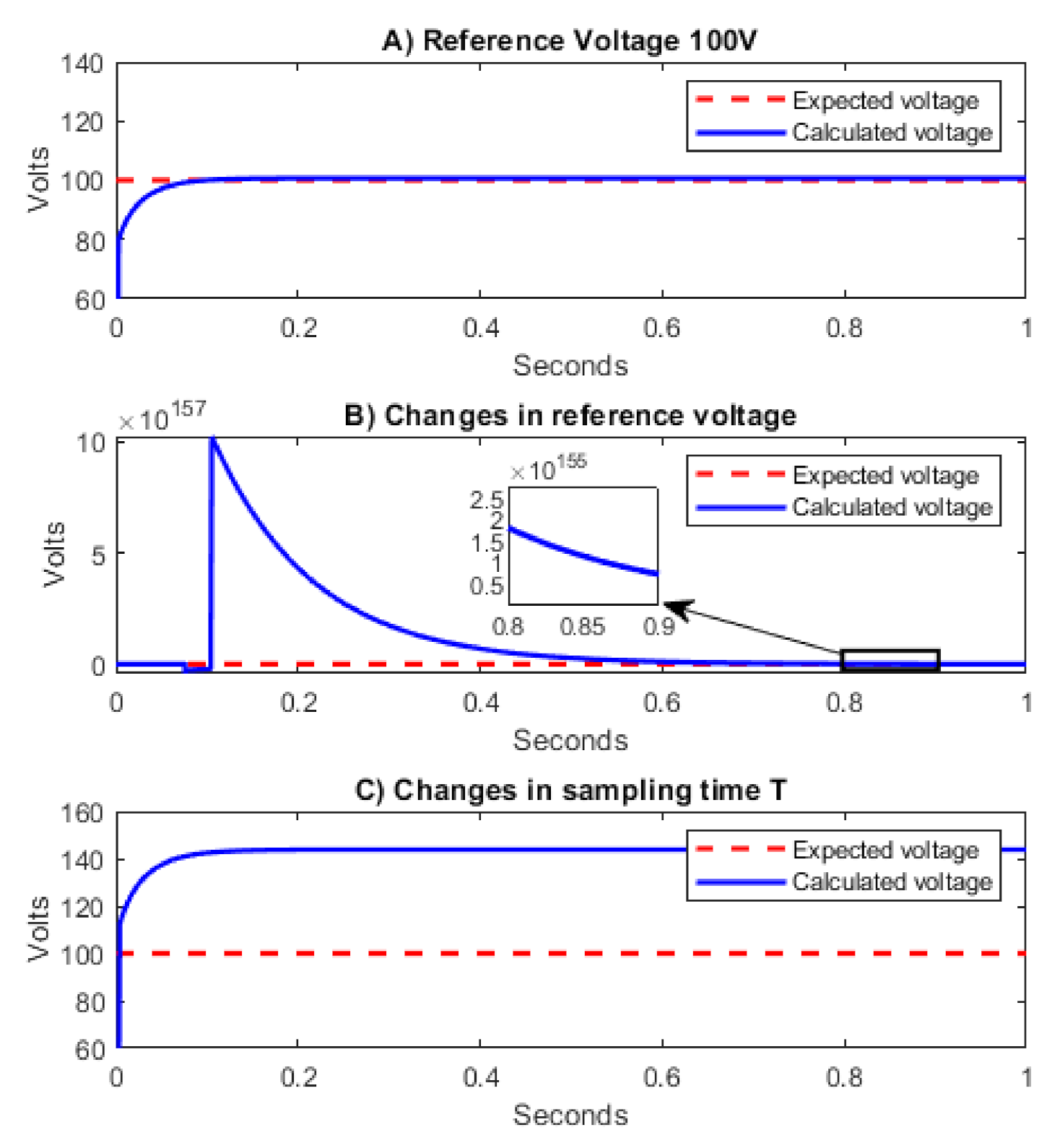
Figure 2a shows the implementation of the inverse optimal control with a reference voltage of
V with
%, in
Figure 2b, a change in the reference voltage from
to
is applied, and the output voltage never converges to the voltage reference, whose percentage of error reaches values of
%. Finally, in
Figure 2c a change in the sampling time from
to
is applied to generate a percentage error
%.
.
Figure 2 shows that the method fails when a simple change is made in the voltage reference and the error increases when a change is made in the sampling time
. Therefore, the inverse optimal control used in the works [
24,
25,
26,
33,
34,
35] is unable to solve these problems without making a change in Equation (14).
7. Conclusions
In this paper, a new inverse optimal control for a boost converter has been developed. Besides, a new method to tune the inverse optimal control was proposed. Such a method was tested for changes in the reference voltage, also, it was proved that said tuning of the control method has a good response under changes in the input voltage and in the load. Furthermore, based on the results, it can be deduced that the method can help to find a relation of the proposed for the boost converter, subject to changes in the input variables and the given reference, in addition to changes in the system parameters. In our case, there is a linear type relation, to expand the robustness of the model in the face of changes in the voltage reference, which ensures the stability of our system. Taking the amplitude of each interval and comparing the lower and upper limits of each variable, at which the new control methodology was tested in our system. Said coefficient of linear adjustment was able to damp, an amplitude of 50 V for the reference voltage, corresponding to a change of 50%. An amplitude of 250 corresponding to a 500% change in load. It was tested with an input voltage variation of 120%. For capacitance, an amplitude of 5 corresponding to a change of 55% and for inductance an amplitude of corresponding to changes of up to 300%. Whose system stability was preserved, with an error of less than 1% according to the voltage reference. Simulation results probe the effectiveness of our proposed control methodology.


