Drying of Sisal Fiber: A Numerical Analysis by Finite-Volumes

Abstract

Vegetable fibers have inspired studies in academia and industry, because of their good characteristics appropriated for many technological applications. Sisal fibers (Agave sisalana variety), when extracted from the leaf, are wet and must be dried to reduce moisture content, minimizing deterioration and degradation for long time. The control of the drying process plays an important role to guarantee maximum quality of the fibers related to mechanical strength and color. In this sense, this research aims to evaluate the drying of sisal fibers in an oven with mechanical air circulation. For this purpose, a transient and 3D mathematical model has been developed to predict moisture removal and heating of a fiber porous bed, and drying experiments were carried out at different drying conditions. The advanced model considers bed porosity, fiber and bed moisture, simultaneous heat and mass transfer, and heat transport due to conduction, convection and evaporation. Simulated drying and heating curves and the hygroscopic equilibrium moisture content of the sisal fibers are presented and compared with the experimental data, and good concordance was obtained. Results of moisture content and temperature distribution within the fiber porous bed are presented and discussed in details. It was observed that the moisture removal and temperature kinetics of the sisal fibers were affected by the temperature and relative humidity of the drying air, being more accentuated at higher temperature and lower relative humidity, and the drying process occurred in a falling rate period.

1. Introduction

Vegetable fibers originate from plants and, basically, are composed of a solid skeleton and pores filled with fluid. The major components of these materials are cellulose, hemicellulose and lignin, with minor percentages of pectin, proteins, wax, inorganic salts and other water-soluble substances. Based on the cultivation region, soil type and climatic conditions, the chemical composition of vegetable fibers present some differences in values [1]. In Brazil, there are large varieties of vegetable fibers, for example: caroá, macambira, curauá, pineapple leaf, jute, cotton, and sisal.

Sisal (Agave sisalana perrine) is a plant cultivated in semiarid regions, resistant to aridity and strong solar irradiation. The leaf of sisal contains about 4% fiber, 1% film (cuticle), 8% dry matter and 87% water. After the fiber is extracted, the rest of the materials are processing waste, frequently used for different purposes, for example, as organic fertilizer, animal feed and by the pharmaceutical industry [2,3].

The sisal fiber when extracted from the leaf is moist. Thus, these biological materials must be dried, in order to avoid deterioration and to be used for most purposes. Green sisal fibers have a color that varies from white to light yellow, but it soon becomes discolored, turning a creamy-white or dark yellow, when submitted to intense heating for long time. However, the sisal fiber processing is responsible for more than half a million direct or indirect jobs, such as, activities of crop maintenance, harvesting, leaf cutting, fiber shredding and processing [2]. After processing, the sisal fibers are commonly used in different industrial sectors, such as in the automotive industry, replacing synthetic fibers, and as reinforcement in polymer composite materials. The vast application field of these fibers is due to their various advantages, such as low cost, low density, high specific strength and stiffness, low abrasiveness to process equipment, biodegradability, nontoxicity and nonpollution, significant reduction of environmental problems. Mainly they originate from renewable sources and are found in many regions in the world [4,5,6,7]. Despite the large advantages, these fibers are very susceptible to moisture and temperature actions, which strongly affect their mechanical properties, mainly when used as reinforcement in polymer composite.

Drying is a complex and coupled phenomenon of heat and mass transfer, momentum and sometimes dimensional variations [8]. The drying process control of sisal fibers plays an important role in obtaining the optimized drying conditions. The idea is to reduce product losses and increase energy saving.

According to literature, sisal fiber drying is realized currently by putting the fibers into the oven; however, the monitoring of the moisture and temperature transient behavior along the process is a secondary goal. However, severe changes in the temperature and moisture inside the fibers generate hydric-thermo-mechanical stresses which can cause fiber deterioration, rupture and weakness in the material. Thus, to adequately control drying process is important.

Unfortunately, few works about drying of sisal fibers have been reported in the literature. These works, the majority is focused in experiments [9,10,11,12] while others are dedicated to theoretical analysis by using analytical and numerical procedures [13,14,15,16,17,18,19,20].

Ferreira et al. [9] reported that the cellulose polysaccharide chains are more tightly arranged after moisture removal during drying and, consequently, the microfibrils come together in the dry state as a result of increased packaging. Besides, according to the authors, fiber voids are significantly reduced as consequence of the drying process, and cannot be completely reopened with rehumidification process. The minor water absorption rate minimizes the fiber dimensional changes, resulting in larger fiber dimensional stability.

Santos et al. [10] evaluated the effects of convective drying (in oven) on the mechanical properties of sisal fibers. In this research, they studied the moisture loss and heating processes, and the effect of the drying air conditions on the mechanical properties of these materials. According to the authors, air temperature ranging from 60 to 105 °C significantly affected not the tensile mechanical properties, elongation at rupture and modulus of elasticity of the sisal fibers, but caused discoloration.

Work by Ghosh [12] indicates that artificial drying of sisal fiber, after decortication and squeezing to remove free water, currently is realized in dryers at air temperature ranging from 100–110 °C. However, according to the author, sisal fiber can be dried at temperature of around 180 °C, and inevitable problem such as discoloration can be minimized by adequately controlling drying time and temperature. In this way, it is possible to obtain products with an acceptable quality level.

Diniz et al. [13], in their research related to the drying of sisal fibers, proposed lumped mathematical models to predict the transient behavior of the average moisture content and surface temperature, and also, the equilibrium moisture content of vegetable fiber as a function of the drying air temperature and water vapor concentration in the fiber porous bed. According to the authors, predicted results were in good fit with experimental data; for all drying conditions used correlation coefficients greater than 0.99 were obtained, and thus, was shown the potential of the proposed models to appropriately predict the drying process of sisal fiber, and other related materials.

Nordon and David [17] studied the coupled diffusion of heat and moisture in hygroscopic textile materials. The authors presented a 1D-numerical solution of the governing equations by finite differences, based on the “double scan” method for the nonlinear differential equations. The study was applied to wool, as an example of hygroscopic material and showed that the moisture transfers from the air to the wool and from the wool to the air are not symmetrical processes. According to the authors, the method does not predict the physical problem adequately.

Haghi [18] studied the simultaneous heat and moisture transfer in porous systems. For this purpose and based on the model reported by Nordon and David (1967) [17], the authors developed a one-dimensional mathematical model and its numerical solution using the finite difference method. The effects of operational parameters, such as temperature and moisture in the dryer, the initial moisture content of the porous material and the mass and heat transfer coefficients are examined using this model. The aim of this study was to describe adequately the heat and mass transfer during convective drying. According to the authors the proposed model can be used to predict transient variations in temperature distribution and moisture content in fabrics with reasonable accuracy.

Xiao et al. [19] and Xiao et al. [20] reported studies about mass transfer (imbibition process) in fibrous porous media using the fractal theory including surface roughness. The global model is based on the capillary theory (Hagen–Poiseuille model and Kozeny-Carman equation), assuming that the porous media is formed by a numbers of capillaries tubes. According to the authors, the proposed model predicts adequately the physical mechanisms of fluid transport inside fibrous porous media, and it contains no empirical constant, as commonly required for different models.

As already mentioned in previous comments, different distributed models have been reported in the literature applied to heat and/or mass transfer in fibrous porous media; however, restricted to one-dimensional approaches, no works used the finite volume technique for numerical solution of the governing equations. Then, in complement to these studies, this work aims to study the drying of sisal fibers in an oven using a 3D advanced mathematical modeling that considers the coupled phenomena of heat and mass transport inside the material, including fiber bed porosity and sorption heat. Here, the finite-volumes numerical method has been used to solve the governing equations. The idea is to assist engineers, industrials and academics in a rigorous understanding of the dominant mechanisms involved in the diffusion process occurring in the drying process.

2. Methodology

2.1. Mathematical Modeling

2.1.1. Geometry and the Physical Problem

In this paper, the physical problem consists in predicting the moisture and heat transfer within a wet fibrous medium in the shape of a rectangular prism, as illustrated in the Figure 1. The fibrous medium is formed by a series of rigid and nonreactive fibers. In the drying process, hot air flows around the porous bed supplying heat to the wet fibers. The physical effect is to evaporate water inside the fiber, to heat the fibers, and to remove the water in the vapor phase. Water molecules in the vapor phase are free to move between the voids through the fiber bed, and to be absorbed or desorbed by the fibers. Volume variations provoked by water removal and heating of the fiber are not considered.

2.1.2. The Governing Equations

Vapor Diffusion Equation

To predict the water vapor concentration behavior inside the fiber bed along the drying process, the following equation was considered:

$$\left[\mathsf{\epsilon }+\left(1-\mathsf{\epsilon }\right){\mathsf{\rho }}_{\mathrm{s}} \mathsf{\sigma }\right]\frac{\partial \mathrm{C}}{\partial \mathrm{t}}=\left[ \frac{\partial }{\partial \mathrm{x}}\left(\mathrm{D}\frac{\partial \mathrm{C}}{\partial \mathrm{x}}\right)+\frac{\partial }{\partial \mathrm{y}}\left(\mathrm{D}\frac{\partial \mathrm{C}}{\partial \mathrm{y}}\right)+\frac{\partial }{\partial \mathrm{z}}\left(\mathrm{D}\frac{\partial \mathrm{C}}{\partial \mathrm{z}}\right)\right]+\left(1-\mathsf{\epsilon }\right){\mathsf{\rho }}_{\mathrm{s}} \mathsf{\beta } \frac{\partial \mathrm{T}}{\partial \mathrm{t}},$$

(1)

where $\mathsf{\sigma }$ and $\mathsf{\beta }$ are constants from the equilibrium equation; ε is the porosity; ${\mathsf{\rho }}_{\mathrm{s}}$ is the fiber density; $\mathrm{C}$ is the water vapor concentration (interfibers); T is the temperature, and t is the time. The parameter $\mathrm{D}=\mathsf{\epsilon }\mathrm{D}\prime$ and $\mathrm{D}\prime$ represents the vapor diffusion coefficient within the fibrous medium. In Equation (1), it is clear the effect of heat transfer in the mass transfer phenomenon.

In the model, the following initial and boundary conditions were adopted:

• Initial condition:

$$\mathrm{C}\left(\mathrm{x},\mathrm{y},\mathrm{z},\mathrm{t}=0\right)={\mathrm{C}}_{\mathrm{o}},$$

(2)

• Boundary conditions:

$$-\mathrm{D}{\frac{\partial \mathrm{C}}{\partial \mathrm{x}}|}_{\mathrm{x}={\mathrm{R}}_1}={\mathrm{h}}_{\mathrm{mx}}\left(\mathrm{C}-{\mathrm{C}}_{\mathrm{eq}}\right), \forall \left(\mathrm{x}={\mathrm{R}}_1, \mathrm{y}, \mathrm{z}, \mathrm{t}>0\right);$$

(3)

$$-\mathrm{D}{\frac{\partial \mathrm{C}}{\partial \mathrm{y}}|}_{\mathrm{y}={\mathrm{R}}_2}={\mathrm{h}}_{\mathrm{my}}\left(\mathrm{C}-{\mathrm{C}}_{\mathrm{eq}}\right), \forall \left(\mathrm{x}, \mathrm{y}={\mathrm{R}}_2,\mathrm{z}, \mathrm{t}>0\right);$$

(4)

$$-\mathrm{D}{\frac{\partial \mathrm{C}}{\partial \mathrm{z}}|}_{\mathrm{z}={\mathrm{R}}_3}={\mathrm{h}}_{\mathrm{mz}}\left(\mathrm{C}-{\mathrm{C}}_{\mathrm{eq}}\right), \forall \left(\mathrm{x}, \mathrm{y},\mathrm{z}={\mathrm{R}}_3, \mathrm{t}>0\right).$$

(5)

Heat Conduction Equation

To predict the temperature of the fibers bed along the drying process, the following energy equation was used:

$$\mathsf{\rho }\left({\mathrm{c}}_{\mathrm{P}}+{ \mathrm{h}}_{\mathrm{s}}\mathsf{\beta }\right)\frac{\partial \mathrm{T}}{\partial \mathrm{t}}=\left[\frac{\partial }{\partial \mathrm{x}}\left( \mathrm{K}\frac{\partial \mathrm{T}}{\partial \mathrm{x}}\right)+\frac{\partial }{\partial \mathrm{y}}\left(\mathrm{K}\frac{\partial \mathrm{T}}{\partial \mathrm{y}}\right)+\frac{\partial }{\partial \mathrm{z}}\left( \mathrm{K}\frac{\partial \mathrm{T}}{\partial \mathrm{z}}\right)\right]+{ \mathrm{h}}_{\mathrm{s}} \mathsf{\rho } \mathsf{\sigma }\frac{\partial \mathrm{C}}{\partial \mathrm{t}},$$

(6)

where ${\mathrm{c}}_{\mathrm{p}}$ is the specific heat; K is the thermal conductivity; ${\mathrm{h}}_{\mathrm{s}}$ is the enthalpy and, T is the temperature. In Equation (6), it is considered that the energy of the wet air inside the fiber bed is negligible compared to the energy of the fibers. In Equation (6), the effect of mass transfer in the heat transfer phenomenon is clear.

• Initial condition:

$$\mathrm{T}\left(\mathrm{x},\mathrm{y},\mathrm{z},\mathrm{t}=0\right)={\mathrm{T}}_{\mathrm{o}}.$$

(7)

• Boundary conditions for heat transfer:

$$-\mathrm{K}{\frac{\partial \mathrm{T}}{\partial \mathrm{x}}|}_{\mathrm{x}={\mathrm{R}}_1}={\mathrm{h}}_{\mathrm{cx}}\left(\mathrm{T}-{\mathrm{T}}_{\mathrm{eq}}\right),\forall \left(\mathrm{x}={\mathrm{R}}_1, \mathrm{y}, \mathrm{z}, \mathrm{t}>0\right);$$

(8)

$$-\mathrm{K}{\frac{\partial \mathrm{T}}{\partial \mathrm{y}}|}_{\mathrm{y}={\mathrm{R}}_2}={\mathrm{h}}_{\mathrm{cy}}\left(\mathrm{T}-{\mathrm{T}}_{\mathrm{eq}}\right),\forall \left(\mathrm{x}, \mathrm{y}={\mathrm{R}}_2,\mathrm{z}, \mathrm{t}>0\right);$$

(9)

$$-\mathrm{K}{\frac{\partial \mathrm{T}}{\partial \mathrm{z}}|}_{\mathrm{z}={\mathrm{R}}_3}={\mathrm{h}}_{\mathrm{cz}}\left(\mathrm{T}-{\mathrm{T}}_{\mathrm{eq}}\right),\forall \left(\mathrm{x}, \mathrm{y},\mathrm{z}={\mathrm{R}}_3, \mathrm{t}>0\right).$$

(10)

Λ Equilibrium Equation

According to Crank [21], the following equilibrium equation was considered:

$$\mathrm{M}= \mathsf{\alpha }+\mathsf{\sigma }\mathrm{C}-\mathsf{\beta }\mathrm{T},$$

(11)

where $\mathrm{M}$ is the moisture absorbed per unit mass of fiber (${\mathrm{kg}}_{\mathrm{vapor}}/{\mathrm{kg}}_{\mathrm{dry} \mathrm{fiber}})$, and $\mathsf{\alpha }, \mathsf{\sigma }$ and $\mathsf{\beta }$ are constants, that can be obtained by fitting to experimental data.

From Equation (11), it is possible to obtain the following derivative:

$$\frac{\partial \mathrm{M}}{\partial \mathrm{t}}=\mathsf{\sigma }\frac{\partial \mathrm{C}}{\partial \mathrm{t}}-\mathsf{\beta }\frac{\partial \mathrm{T}}{\partial \mathrm{t}}$$

(12)

The average value of the potential of interest can be determined as follows:

$$\overline{\mathsf{\Phi }}=\frac{1}{\mathrm{V}}{{\displaystyle \int }}_{\mathrm{V}}\mathsf{\Phi }\mathrm{d}V,$$

(13)

where Φ can be C, T or M (Equation (11)) and V is the volume of the fibrous medium.

2.2. Numerical Procedure

Equations (1) and (6) are highly nonlinear differential equations. Thus, exact solutions of these equation isn´t possible. Thus, in this paper, these equations are solved using the finite-volume method [22,23,24]. In the discretization process, the following assumptions were adopted:

(a)

The solid is homogeneous and isotropic;

(b)

The only mechanism of water transport within the solid is diffusion;

(c)

The thermophysical parameters are constant along the drying process;

(d)

The diffusion coefficient is constant along the drying;

(e)

Convective mass and heat transfer coefficients are constant along the drying.

Due to the geometric shape (rectangular prism), it is possible to numerically solve the physical problem treated here using only one symmetrical part of the domain, as illustrated in Figure 2. In Figure 3 is shown the computational domain utilized in the discretization process of the governing equation.

Based on the Figure 3, and integrating Equation (1) into volume and time, the following linear algebraic equation is obtained for the internal control volumes P:

$${\mathrm{A}}_{\mathrm{p}}{\mathrm{C}}_{\mathrm{P} }={\mathrm{A}}_{\mathrm{e}}{\mathrm{C}}_{\mathrm{E} }+{\mathrm{A}}_{\mathrm{w}}{\mathrm{C}}_{\mathrm{W} }+{\mathrm{A}}_{\mathrm{n}}{\mathrm{C}}_{\mathrm{N} }+{\mathrm{A}}_{\mathrm{s}}{\mathrm{C}}_{\mathrm{S}}+{\mathrm{A}}_{\mathrm{f}}{\mathrm{C}}_{\mathrm{F} }+{\mathrm{A}}_{\mathrm{b}}{\mathrm{C}}_{\mathrm{B}}+\mathrm{B},$$

(14)

where,

$${\mathrm{A}}_{\mathrm{p}}=\left[\mathsf{\epsilon }+\left(1-\mathsf{\epsilon }\right){\mathsf{\rho }}_{\mathrm{s}} \mathsf{\sigma }\right] \frac{\Delta \mathrm{x}\Delta \mathrm{y}\Delta \mathrm{z}}{\Delta \mathrm{t}}+{ \mathrm{D}}_{\mathrm{e}}^{\mathrm{C}}\frac{\Delta \mathrm{y}\Delta \mathrm{z}}{{\mathsf{\delta }\mathrm{x}}_{\mathrm{e}}}+{ \mathrm{D}}_{\mathrm{w}}^{\mathrm{C}}\frac{\Delta \mathrm{y}\Delta \mathrm{z}}{{\mathsf{\delta }\mathrm{x}}_{\mathrm{w} }}+{ \mathrm{D}}_{\mathrm{n}}^{\mathrm{C}}\frac{\Delta \mathrm{x}\Delta \mathrm{z}}{{\mathsf{\delta }\mathrm{y}}_{\mathrm{n}}}+{\mathrm{D}}_{\mathrm{s}}^{\mathrm{C}}\frac{\Delta \mathrm{x}\Delta \mathrm{z}}{{\mathsf{\delta }\mathrm{y}}_{\mathrm{s}}}+{ \mathrm{D}}_{\mathrm{f}}^{\mathrm{C}}\frac{\Delta \mathrm{x}\Delta \mathrm{y}}{{\mathsf{\delta }\mathrm{z}}_{\mathrm{f}}}+{ \mathrm{D}}_{\mathrm{b}}^{\mathrm{C}}\frac{\Delta \mathrm{x}\Delta \mathrm{y}}{{\mathsf{\delta }\mathrm{z}}_{\mathrm{b}}},$$

(15)

$${\mathrm{A}}_{\mathrm{e}}={ \mathrm{D}}_{\mathrm{e}}^{\mathrm{C}}\frac{\Delta \mathrm{y}\Delta \mathrm{z}}{{\mathsf{\delta }\mathrm{x}}_{\mathrm{e}}},$$

(16)

$${\mathrm{A}}_{\mathrm{w}}={ \mathrm{D}}_{\mathrm{w}}^{\mathrm{C}}\frac{\Delta \mathrm{y}\Delta \mathrm{z}}{{\mathsf{\delta }\mathrm{x}}_{\mathrm{w} }},$$

(17)

$${\mathrm{A}}_{\mathrm{n}}={ \mathrm{D}}_{\mathrm{n}}^{\mathrm{C}}\frac{\Delta \mathrm{x}\Delta \mathrm{z}}{{\mathsf{\delta }\mathrm{y}}_{\mathrm{n}}},$$

(18)

$${\mathrm{A}}_{\mathrm{s}}={ \mathrm{D}}_{\mathrm{s}}^{\mathrm{C}}\frac{\Delta \mathrm{x}\Delta \mathrm{z}}{{\mathsf{\delta }\mathrm{y}}_{\mathrm{s}}},$$

(19)

$${\mathrm{A}}_{\mathrm{f}}={ \mathrm{D}}_{\mathrm{f}}^{\mathrm{C}}\frac{\Delta \mathrm{x}\Delta \mathrm{y}}{{\mathsf{\delta }\mathrm{z}}_{\mathrm{f}}},$$

(20)

$${\mathrm{A}}_{\mathrm{b}}={ \mathrm{D}}_{\mathrm{b}}^{\mathrm{C}}\frac{\Delta \mathrm{x}\Delta \mathrm{y}}{{\mathsf{\delta }\mathrm{z}}_{\mathrm{b}}},$$

(21)

$$\mathrm{B}=\left[\mathsf{\epsilon }+\left(1-\mathsf{\epsilon }\right){\mathsf{\rho }}_{\mathrm{s}} \mathsf{\sigma }\right]\frac{\Delta \mathrm{x}\Delta \mathrm{y}\Delta \mathrm{z}}{\Delta \mathrm{t}}{\mathrm{C}}_{\mathrm{P}}^0+{\mathrm{S}}^{\mathrm{C}} \Delta \mathrm{x}\Delta \mathrm{y}\Delta \mathrm{z}.$$

(22)

For boundary volumes, the integration process of the governing equation is similar, as described for the internal points. However, must be considered the existing boundary conditions. For example, considering the symmetry condition, the mass fluxes in the west, back and south faces are null, i.e., ${\mathrm{C}}_{\mathrm{w}}^{″}=0,{ \mathrm{C}}_{\mathrm{b}}^{″}=0$ and ${\mathrm{C}}_{\mathrm{s}}^{″}=0$, as illustrated in Figure 4.

For the heat transfer equation after integration procedure, the following discretized linear algebraic equation is obtained:

$${\mathrm{A}}_{\mathrm{p}}{\mathrm{T}}_{\mathrm{P} }={\mathrm{A}}_{\mathrm{e}}{\mathrm{T}}_{\mathrm{E} }+{\mathrm{A}}_{\mathrm{w}}{\mathrm{T}}_{\mathrm{W} }+{\mathrm{A}}_{\mathrm{n}}{\mathrm{T}}_{\mathrm{N} }+{\mathrm{A}}_{\mathrm{s}}{\mathrm{T}}_{\mathrm{S}}+{\mathrm{A}}_{\mathrm{f}}{\mathrm{T}}_{\mathrm{F} }+{\mathrm{A}}_{\mathrm{b}}{\mathrm{T}}_{\mathrm{B}}+\mathrm{B},$$

(23)

where,

$${\mathrm{A}}_{\mathrm{p}}=\frac{\mathsf{\rho }\left({\mathrm{c}}_{\mathrm{P}}+{\mathrm{h}}_{\mathrm{s}}\mathsf{\beta }\right)\Delta \mathrm{x}\Delta \mathrm{y}\Delta \mathrm{z}}{\Delta \mathrm{t}}+{ \mathrm{K}}_{\mathrm{e}}^{\mathrm{T}}\frac{\Delta \mathrm{y}\Delta \mathrm{z}}{{\mathsf{\delta }\mathrm{x}}_{\mathrm{e}}}+{ \mathrm{K}}_{\mathrm{w}}^{\mathrm{T}}\frac{\Delta \mathrm{y}\Delta \mathrm{z}}{{\mathsf{\delta }\mathrm{x}}_{\mathrm{w} }}+{\mathrm{K}}_{\mathrm{n}}^{\mathrm{T}}\frac{\Delta \mathrm{x}\Delta \mathrm{z}}{{\mathsf{\delta }\mathrm{y}}_{\mathrm{n}}}+{\mathrm{K}}_{\mathrm{b}}^{\mathrm{T}}\frac{\Delta \mathrm{x}\Delta \mathrm{z}}{{\mathsf{\delta }\mathrm{y}}_{\mathrm{s}}}+{ \mathrm{K}}_{\mathrm{f}}^{\mathrm{T}}\frac{\Delta \mathrm{x}\Delta \mathrm{y}}{{\mathsf{\delta }\mathrm{z}}_{\mathrm{f}}}+{ \mathrm{K}}_{\mathrm{b}}^{\mathrm{T}}\frac{\Delta \mathrm{x}\Delta \mathrm{y}}{{\mathsf{\delta }\mathrm{z}}_{\mathrm{b}}},$$

(24)

$${\mathrm{A}}_{\mathrm{e}}={ \mathrm{K}}_{\mathrm{e}}^{\mathrm{T}}\frac{\Delta \mathrm{y}\Delta \mathrm{z}}{{\mathsf{\delta }\mathrm{x}}_{\mathrm{e}}},$$

(25)

$${\mathrm{A}}_{\mathrm{w}}={ \mathrm{K}}_{\mathrm{w}}^{\mathrm{T}}\frac{\Delta \mathrm{y}\Delta \mathrm{z}}{{\mathsf{\delta }\mathrm{x}}_{\mathrm{w} }},$$

(26)

$${\mathrm{A}}_{\mathrm{n}}={\mathrm{K}}_{\mathrm{n}}^{\mathrm{T}}\frac{\Delta \mathrm{x}\Delta \mathrm{z}}{{\mathsf{\delta }\mathrm{y}}_{\mathrm{n}}},$$

(27)

$${\mathrm{A}}_{\mathrm{s}}={ \mathrm{K}}_{\mathrm{s}}^{\mathrm{T}}\frac{\Delta \mathrm{x}\Delta \mathrm{z}}{{\mathsf{\delta }\mathrm{y}}_{\mathrm{s}}},$$

(28)

$${ \mathrm{A}}_{\mathrm{f}}={ \mathrm{K}}_{\mathrm{f}}^{\mathrm{T}}\frac{\Delta \mathrm{x}\Delta \mathrm{y}}{{\mathsf{\delta }\mathrm{z}}_{\mathrm{f}}},$$

(29)

$${ \mathrm{A}}_{\mathrm{b}}={ \mathrm{K}}_{\mathrm{b}}^{\mathrm{T}}\frac{\Delta \mathrm{x}\Delta \mathrm{y}}{{\mathsf{\delta }\mathrm{z}}_{\mathrm{b}}},$$

(30)

$$\mathrm{B}=\frac{\mathsf{\rho }\left({\mathrm{c}}_{\mathrm{P}}+{\mathrm{h}}_{\mathrm{s}}\mathsf{\beta }\right) \Delta \mathrm{x}\Delta \mathrm{y}\Delta \mathrm{z}}{\Delta \mathrm{t}}{\mathrm{T}}_{\mathrm{P}}^0+{\mathrm{S}}^{\mathrm{T}} \Delta \mathrm{x}\Delta \mathrm{y}\Delta \mathrm{z}.$$

(31)

In the discretized form, Equation (6) applied to vapor concentration assumes the form:

$$\overline{\mathrm{C}}=\frac{1}{\mathrm{V}}{\displaystyle \sum }_{\mathrm{i}=2}^{\mathrm{npx}-1} {\displaystyle \sum }_{\mathrm{j}=2}^{\mathrm{npy}-1} {\displaystyle \sum }_{\mathrm{k}=2}^{\mathrm{npz}-1}{\mathrm{C}}_{\mathrm{ijk}}\Delta {\mathrm{V}}_{\mathrm{ijk}}^{\prime } ,$$

(32)

where,

$$\mathrm{V}={\displaystyle \sum }_{\mathrm{i}=2}^{\mathrm{npx}-1} {\displaystyle \sum }_{\mathrm{j}=2}^{\mathrm{npy}-1} {\displaystyle \sum }_{\mathrm{k}=2}^{\mathrm{npz}-1}\Delta {\mathrm{V}}_{\mathrm{ijk}}^{\prime } ,$$

(33)

where i, j and k define the position nodal point, $\Delta {\mathrm{V}}_{\mathrm{ijk}}^{\prime }=\Delta \mathrm{x}\Delta \mathrm{y}\Delta \mathrm{z}$ is the volume of the elemental volume, and npx-2, npy-2, and npz-2 are the number of control volumes in the x, y, and z directions, respectively.

To solve iteratively (Gauss–Seidel method) the systems of algebraic equations originated from the Equations (14) and (23) as applied for all control-volume, a computational code using Mathematica^® software was developed. In the numerical treatment, the following convergence criterion was used at each nodal point and process time:

$$\left|{\mathsf{\Phi }}^{\mathrm{n}+1}-{\mathsf{\Phi }}^{\mathrm{n}}\right|\le {10}^{-8},$$

(34)

where $\mathsf{\Phi }$ can be C or T, and n represents the nth iteration at each time point. Simulations were performed using a numerical mesh of 20 × 20 × 20 nodal points and ∆t = 20s, which were obtained after a rigorous mesh and time step refining study.

2.3. Experimental Study

In this work, sisal fibers (Agave sisalana variety) were used in the drying experiments. The wet fibers were obtained in a farm located close to the town of Pocinhos, State of Paraiba, Brazil. The fibers were submitted to drying in oven with forced air circulation at different operating conditions. In Figure 5 is shown the sisal fibers bed used in the experiment.

Table 1. Experimental conditions of air and sisal fiber.

Air			Fibrous Medium							Process Time
RH (%)	T (°C)	v (m/s)	2R1 (m)	2R2 (m)	2R3 (m)	Mo (d.b.)	Meq (d.b.)	To (°C)	Tf (°C)	t (h)
17.52	50	0.05	0.1	0.05	0.1	0.11327	0.03837	29.8	46.3	7.7
11.04	60	0.06	0.1	0.05	0.1	0.11118	0.02606	29.8	56.6	6.7
6.89	70	0.07	0.1	0.05	0.1	0.11148	0.02015	31.5	67.3	5.7
4.19	80	0.08	0.1	0.05	0.1	0.11030	0.01390	29.6	76.3	5.0
3.28	90	0.09	0.1	0.05	0.1	0.11342	0.00525	30.4	87.4	4.7

summarizes information about the fiber and drying air.

In each drying experiments, the sample were withdraw from the oven periodically. In each step, the mass of was evaluated using a digital electronic device (0.001 g precision), and the surface temperature was measured using an infrared thermometer. These measurements were taken every 5 min (about 30 min), after 10, 15, 20, 25 and 30 min time intervals. After this period, the measurements were taken every 60 min until that constant mass was reached. Following that, the sample was dried for 24 h at the same drying temperature, in order to obtain the sample mass at the equilibrium condition, and then for a further 24 h at 105 °C to obtain the dried sample mass. Furthermore, at every measurement instant, temperature and relative humidity of the air outside of the oven were measured. This information was used to calculate air relative humidity inside the oven. In each drying experiments, air velocity inside the oven was measured using a hot wire anemometer. Figure 5 illustrates the point where surface temperatures were taking.

2.4. Parameters Estimation

2.4.1. Transport Coefficients

In this research, the estimation of the mass diffusion coefficient and convective heat and mass transfer coefficients was performed using the least square error technique. Deviations between experimental and predicted values and variance were determined by [25]:

$$\mathrm{ERMQ}={\displaystyle \sum }_{\mathrm{i}=1}^{\mathrm{n}}{\left({\mathsf{\Phi }}_{\mathrm{i}, \mathrm{Num}}-{\mathsf{\Phi }}_{\mathrm{i}, \mathrm{Exp}}\right)}^2,$$

(35)

$${\overline{\mathrm{S}}}^2=\frac{\mathrm{ERMQ}}{\left(\mathrm{n}-\hat{\mathrm{n}}\right)},$$

(36)

where n is the number of experimental points, $\hat{\mathrm{n}}$ is the number of fitted parameters, and Φ can be $\overline{\mathrm{M}}$ or T.

The initial guess of the convective heat transfer coefficient was determined by common correlations for the average Nusselt, Reynolds and Prandtl numbers [26], applied to air flowing over a plane plate by:

$${\mathrm{h}}_{\mathrm{c}}^{\prime }{}_{\mathrm{j}}=\frac{{\overline{\mathrm{Nu}}}_{\mathrm{j}}\times \mathrm{k}}{{\mathrm{R}}_{\mathrm{j}}},$$

(37)

where, ${\overline{\mathrm{Nu}}}_{\mathrm{j}}=0.664\times { \mathrm{Re}}_{\mathrm{j}}{}^{\raisebox{1ex}{$1$}\!\left/ \!\raisebox{-1ex}{$2 $}\right.}\times {\mathrm{Pr}}^{\raisebox{1ex}{$1$}\!\left/ \!\raisebox{-1ex}{$3 $}\right.}$, ${\mathrm{Re}}_{\mathrm{j}}=\frac{\mathsf{\rho }\times \mathrm{v}\times {\mathrm{R}}_{\mathrm{j}}}{\mathsf{\mu }}$, k is the air thermal conductivity and j = 1,2 and 3 (Figure 2), valid in the intervals $5\times {10}^5<\mathrm{Re}\le 1\times {10}^8$.

The initial guess of the convective mass transfer coefficient applied to the air was determined by common correlations for average Sherwood numbers and Schmidt, by [26]:

$${\mathrm{h}}_{\mathrm{m}}^{\prime }{}_{\mathrm{j}}=\frac{{\overline{\mathrm{Sh}}}_{\mathrm{j}}\times {\mathrm{D}}_{\mathrm{AB}}}{{\mathrm{R}}_{\mathrm{j}}},$$

(38)

where, ${\overline{\mathrm{Sh}}}_{\mathrm{j}}=0.664\times {\mathrm{Re}}_{\mathrm{j}}{}^{\raisebox{1ex}{$1$}\!\left/ \!\raisebox{-1ex}{$2 $}\right.}\times {\mathrm{Sc}}^{\raisebox{1ex}{$1$}\!\left/ \!\raisebox{-1ex}{$3 $}\right.}$ and ${\mathrm{D}}_{\mathrm{AB}}$ is the diffusivity of water vapor in the air.

2.4.2. Equilibrium Equation

Considers the Equation (11) re-written in the form:

$$\mathrm{M}={ \mathrm{a}}_1+{\mathrm{a}}_2\times \mathrm{T},$$

(39)

where ${\mathrm{a}}_1=\mathsf{\alpha }+\mathsf{\sigma }\times \mathrm{C}$ and ${\mathrm{a}}_2=-\mathsf{\beta }$.

With the values of T_eq and M_eq for each experimental condition, a linear fit of Equation (39) to the experimental data was performed by the quasi-Newton method using the Statistica^® Software (convergence criterion 9.9 × 10⁻⁵). After this statistical procedure the values of the parameters ${\mathrm{a}}_1$ and ${\mathrm{a}}_2$ were obtained.

On the other hand, considering the drying air as an ideal gas, the air density inside the fibrous bed was calculated by:

$${\mathsf{\rho }}_{\mathrm{air}}=\frac{\mathrm{P}}{\overline{\mathrm{R}}\times {\mathrm{T}}_{\mathrm{abs}}},$$

(40)

where P is the atmospheric pressure, ${\mathsf{\rho }}_{\mathrm{air}}$ is the air density, $\overline{\mathrm{R}}$ is the particular gas constant (atmospheric air), and T_abs is the absolute temperature of the drying-air.

Then, from Equation (40), the equilibrium water vapor concentration between the fibers, can be determined by:

$${\mathrm{C}}_{\mathrm{eq}}={\mathsf{\rho }}_{\mathrm{air}}\times \mathrm{AH},$$

(41)

where AH is the air absolute humidity on the voids of the porous bed.

2.4.3. Estimation of the Fiber and Sample Parameters

The apparent density of the fiber bed was calculated by:

$${\mathsf{\rho }}_{\mathrm{sample}}=\frac{{\mathrm{m}}_{\mathrm{fiber}}}{{ \mathrm{V}}_{\mathrm{sample}}},$$

(42)

where $\mathrm{V}=2{\mathrm{R}}_1\times 2{\mathrm{R}}_2\times 2{\mathrm{R}}_3$ is the volume of the fiber bed.

To obtain the bed porosity, the following equation was used:

$$\mathsf{\epsilon }=1-\frac{{\mathrm{V}}_{\mathrm{fiber}}}{{ \mathrm{V}}_{\mathrm{sample}}},$$

(43)

where ${\mathrm{V}}_{\mathrm{fiber}}=\mathrm{N}\times \mathrm{L}\times \frac{{\mathsf{\pi }\mathrm{d}}^2}{4}$ is the total volume of fibers, L and d, are the length and diameter of the sisal fiber, respectively, and N represents the number of fibers (Figure 6).

The parameters thermal conductivity and specific heat of the fiber bed were determined as follows:

$${\mathrm{k}}_{\mathrm{sample}}=\left(1-\mathsf{\epsilon }\right)\times { \mathrm{k}}_{\mathrm{fiber}}+\mathsf{\epsilon }\times { \mathrm{k}}_{\mathrm{air}},$$

(44)

and

$${ \mathrm{c}}_{\mathrm{p}}{}_{\mathrm{sample}}=\left(1-\mathsf{\epsilon }\right)\times { \mathrm{c}}_{\mathrm{p}}{}_{\mathrm{fiber}}+\mathsf{\epsilon }\times { \mathrm{c}}_{\mathrm{p}}{}_{\mathrm{air}}$$

(45)

Table 2. Geometrical parameters of the fibers and porous bed before drying for different drying conditions.

T (°C)	Fiber Length (m)	* Fiber Diameter (µm)	** Fiber Volume (nm3)	Numbers of Fibers/Sample (---)	Vfiber (m3)	Vsample (m3)	ε (---)
50	0.1	247	4.789	8539	40.895 × 10−6	5.00 × 10−4	0.918
60	0.1	247	4.789	8190	39.224 × 10−6	5.00 × 10−4	0.922
70	0.1	247	4.789	8490	40.660 × 10−6	5.00 × 10−4	0.919
80	0.1	247	4.789	8627	41.316 × 10−6	5.00 × 10−4	0.917
90	0.1	247	4.789	8869	42.475 × 10−6	5.00 × 10−4	0.915

* Santos [15], ** Calculated by equation.

summarizes the geometrical data of the fiber and samples before drying [11,13,14,15,16].

2.5. Thermophysical Properties of the Materials

2.5.1. For Drying Air

Table 3. Air parameters at atmospheric pressure for different drying conditions.

T (°C)	Parameter
	${\mathsf{\rho }}_{\mathbf{a}\mathbf{i}\mathbf{r}}$ $(\mathbf{kg}/{\mathbf{m}}^3)$	${\mathbf{k}}_{\mathbf{a}\mathbf{i}\mathbf{r}}$ $(\mathbf{W}/\mathbf{m}·\mathbf{K})$	${\mathsf{\mu }}_{\mathbf{a}\mathbf{i}\mathbf{r}}$ $(\mathbf{N}·\mathbf{s}/{\mathbf{m}}^2)$	AHair (kgvapor /kgdry air)	AHair, sat (kgvapor /kgdry air)
50	1.0835	0.0269	19.054 × 10−6	0.01363	0.0863
60	1.0508	0.0276	19.509 × 10−6	0.01387	0.1524
70	1.0204	0.0283	19.966 × 10−6	0.01354	0.2765
80	0.9921	0.0290	20.427 × 10−6	0.01247	0.5464
90	0.9637	0.0296	20.847 × 10−6	0.01449	1.3990
	${\mathrm{D}}_{\mathrm{AB}}$ $\left({\mathrm{m}}^2/\mathrm{s}\right)$	${\mathrm{c}}_{\mathrm{p}}$ $\left(\mathrm{kJ}/\mathrm{kg} \mathrm{K}\right)$	hs (kJ/kg)	Pr (---)	Sc (---)
50	28.06 × 10−6	1.0331	2382.90	0.73210	0.62671
60	29.60 × 10−6	1.0335	2358.34	0.73123	0.62726
70	31.17 × 10−6	1.0335	2333.26	0.73016	0.62774
80	32.78 × 10−6	1.0328	2307.62	0.72884	0.62818
90	34.42 × 10−6	1.0348	2281.39	0.72877	0.62855

and

Table 4. Air dimensionless parameters at atmospheric pressure for different drying conditions.

Dimensionless Parameter	T (°C)
	50	60	70	80	90
${\mathrm{Re}}_{\mathrm{x}}$	142.1625	134.6619	127.7713	121.4225	115.5627
${\mathrm{Re}}_{\mathrm{y}}$	71.0812	67.3309	63.8856	60.7112	57.7813
${\mathrm{Re}}_{\mathrm{z}}$	142.1625	134.6619	127.7713	121.4225	115.5627
${\overline{\mathrm{Nu}}}_{\mathrm{x}}$	7.13539	6.94186	6.75860	6.58460	6.42355
${\overline{\mathrm{Nu}}}_{\mathrm{y}}$	5.04548	4.90864	4.77905	4.65601	4.54213
${\overline{\mathrm{Nu}}}_{\mathrm{z}}$	7.13539	6.94186	6.75860	6.58460	6.42355
${\overline{\mathrm{Sh}}}_{\mathrm{x}}$	6.77511	6.59588	6.42655	6.26630	6.11445
${\overline{\mathrm{Sh}}}_{\mathrm{y}}$	4.79072	4.66399	4.54425	4.43094	4.32357
${\overline{\mathrm{Sh}}}_{\mathrm{z}}$	6.77511	6.59588	6.42655	6.26630	6.11445

present some drying air parameters at atmospheric pressure for each experiments.

2.5.2. For Water and Fiber

Table 5. Sisal fiber parameters and sample for different drying conditions [11,13,14,15,16].

T (°C)	Parameter
	Co (kgvapor/m3)	Ceq (kgvapor/m3)	${\mathsf{\rho }}_{\mathbf{s}\mathbf{a}\mathbf{m}\mathbf{p}\mathbf{l}\mathbf{e}}$ (kg/m3)	${\mathsf{\rho }}_{\mathbf{f}\mathbf{i}\mathbf{b}\mathbf{e}\mathbf{r}}$ (kg/m3)
50	0.04146	0.01482	83.088	1450.00
60	0.04052	0.01458	74.960	1450.00
70	0.04125	0.01381	81.956	1450.00
80	0.04005	0.01439	85.138	1450.00
90	0.4174	0.01403	90.782	1450.00
	${\mathrm{c}}_{\mathrm{p}}{}_{\mathrm{sample}}$ (J/kg·K)	${\mathrm{c}}_{\mathrm{p}}{}_{\mathrm{fiber}}$ (J/kg·K)	${\mathrm{k}}_{\mathrm{sample}}$ (W/m·K)	${\mathrm{k}}_{\mathrm{fiber}}$ (W/m·K)
50	960.8454	149.65	0.03017	0.067
60	964.2007	149.65	0.03067	0.067
70	961.6180	149.65	0.03141	0.067
80	959.8464	149.65	0.03209	0.067
90	959.6211	149.65	0.03278	0.067

presents some fibrous medium parameters for different drying experiments.

3. Results and Discussion

3.1. Fiber Morphology

The scanning electron micrographs (SEM) of untreated sisal fibers in moist condition are illustrated in Figure 7. Upon analyzing this figure, it can be verified that the arrangement of this particular fiber is similar to other natural fibers. It can be seen a spongier aspect, voids, rougher surface and a thin and compacted cellular arrangement. Furthermore, it can be observed that parenchyma cells are widely distributed along the fiber. The fibers presented diameters almost constant along the length and, minor differences between the fibers mean diameter were observed.

3.2. Analysis of Equilibrium Equation

$$\mathrm{M}=0.044702+2.217337\times \mathrm{C}-0.000784\times \mathrm{T}.$$

(46)

Equation (46) predict the linear dependence of the moisture content with the temperature and water vapor concentration, fundamental in predicting the coupling between the Equations (1) and (6). A correlation coefficient R = 0.99 was obtained after the performed linear regression. Most details about the statistical procedure can found in the literature [11,13,14,15,16].

3.3. Moisture Removal and Heat Transfer Analysis

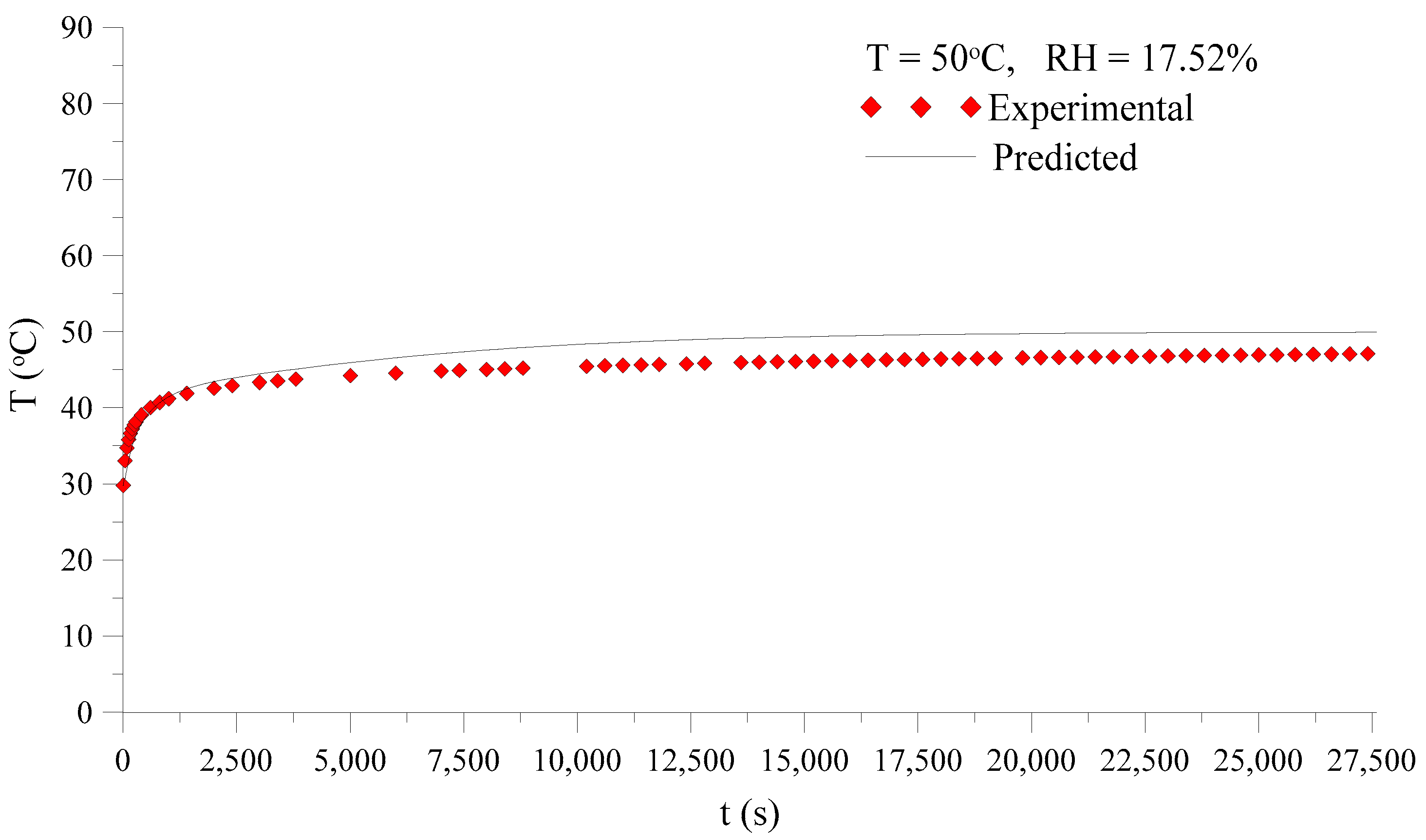
3.3.1. Drying and Heating Kinetics

Figure 8 and Figure 9 illustrate the predicted and experimental average moisture content (dry basis) of the fiber sample as a function of time for the drying air temperature of 50 °C and 80 °C. Upon analyzing these figures, it can be seen that there is a good concordance between the simulated and experimental of the average moisture content along the process for every condition. Besides, it was verified that the average moisture content decreases with time until to reach the hygroscopic equilibrium condition. Furthermore, the drying rate increased and equilibrium moisture content decreased when higher drying air temperature and lower air relative humidity were used in the experiment. Therefore, this physical situation resulted in a short drying time.

In Figure 10 and Figure 11 are shown the comparison between the predicted and experimental transient values of the temperature at the sample surface at 50 °C and 80 °C. Upon analyzing these figures, it can be noted that there is good concordance between surface temperature values in the first 4000 s of process followed by minor discrepancies for long time. For example, in the drying at 50 °C and 27,400 s elapsed time difference, between the predicted and experimental surface temperature data there is 2.8 °C difference, while at 80 °C and 17,800 s elapsed time, the difference in these values is 4.5 °C. These discrepancies may be attributed to minor errors in the temperature measurement procedure in each the experiments or even by the accuracy in the device itself. Besides the differences verified for long time may also be associated with the consideration of constant convective heat coefficient and null dimensional variations along the process as established in the mathematical modeling.

Upon analyzing the Figure 7 and Figure 8, it can be seen that the temperature at the surface of the fibrous bed changed along the drying, reaching the thermal equilibrium condition faster at the highest air temperature. The increases in the surface temperature of the fiber with progress of drying indicates the moisture removal occurred on the falling drying rate period, i.e., the water flux inside the fiber to its surface is less than the water flux removed by the heated air at the surface. Furthermore, it was observed that the fiber temperature increased as the drying rate decreased until the equilibrium condition. These phenomena were cited in the literature [10,11,13,14,15,16].

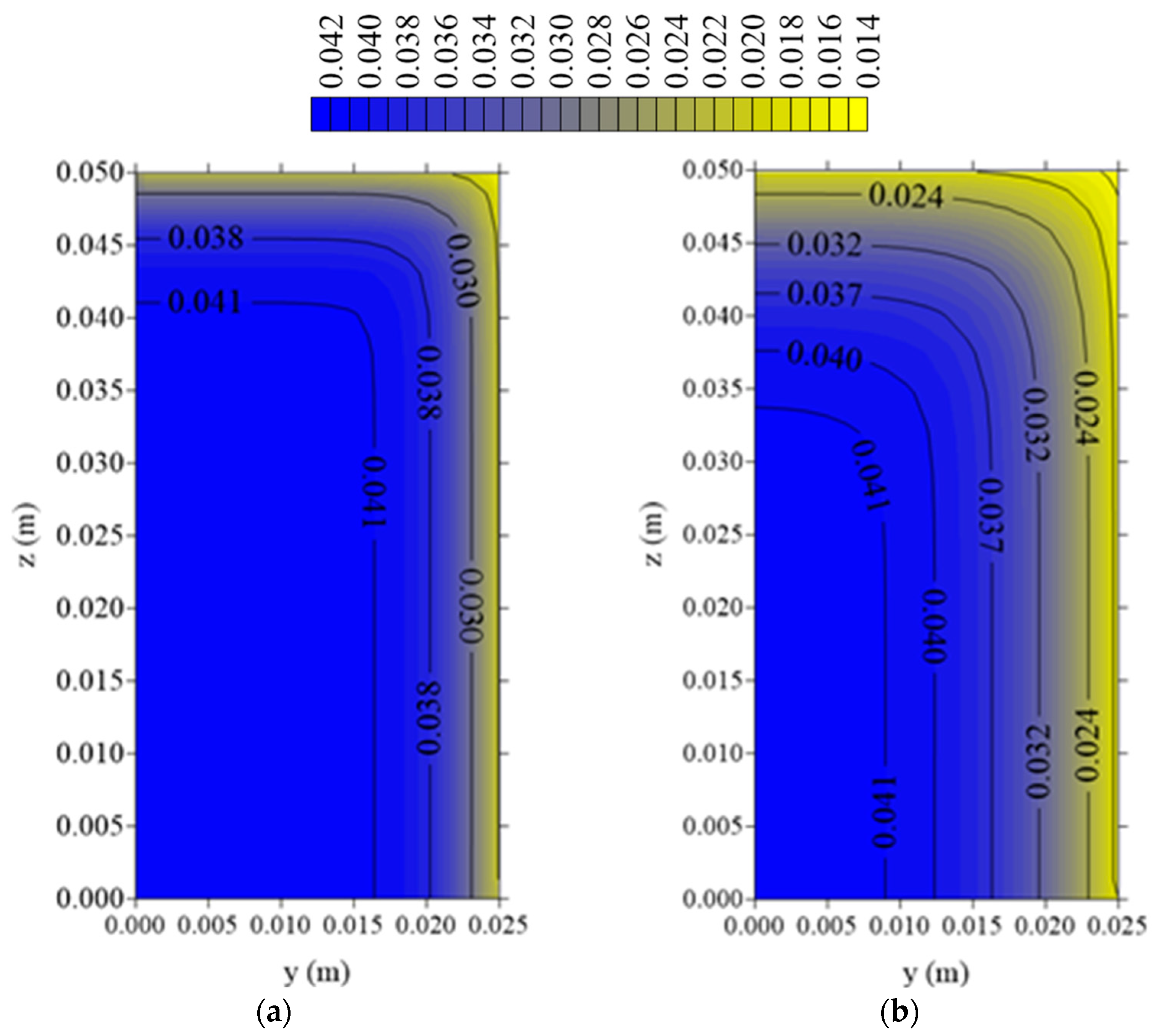
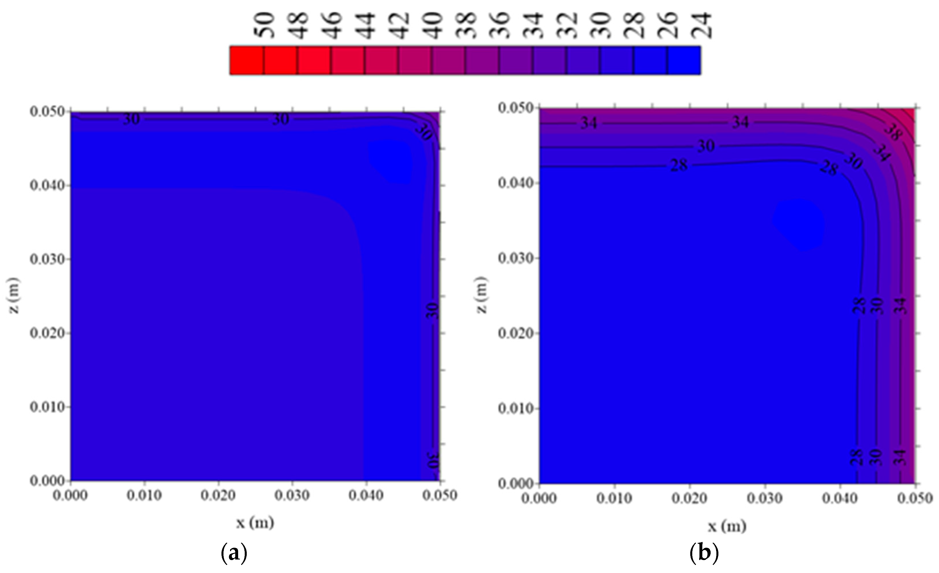
3.3.2. Water Vapor Concentration and Temperature Distributions

In Figure 12 and Figure 13 is illustrated the water vapor concentration field inside the fiber bed, at the plans x = 0.025 m (R₁/2) and y = 0.0125 m (R₂/2), at the moments 200 s, 700 s, 5000 s and 8000 s of the drying process, respectively.

By analyzing the Figure 12 and Figure 13, it is possible to see that water vapor concentration presented the highest values in the center of the fiber bed at any time. Thus, moisture flows from the center to surface. Besides, vapor concentration decreased at any position and time, tending towards its equilibrium condition for long drying time. The regions close to the edge dry faster than the others regions inside the porous bed, especially in the vertex region.

Figure 14 and Figure 15 show the distribution of temperature inside the fiber bed, analyzed in the plans x = 0.025 m (R₁/2) and y = 0.0125 m (R₂/2), at the moments 200 s, 700 s, 5000 s and 8000 s of the drying process, respectively.

Upon analyzing these Fs, it can be seen that the temperature has the lowest results in the center of the fibrous medium along the process. The temperature also increased in any position, tending to the thermal equilibrium condition for long drying time. This behavior proved that heat flux occurs from the surface to the center of the porous sample. Furthermore, it is observed that the maximum temperature occurred close to the edge, especially in the vertex of the sample.

From already mentioned results, the regions close to the vertex dry and heat faster. Therefore, these regions are most susceptible to higher moisture and temperature gradients, which originate hydric and thermal stresses. Based on the intensity of these stresses, the material can achieve unfavorable deformation and rupture levels, and poor quality for a specific application. Under the industrial aspect these results are important to assist engineers in making decision about how the material must be dried and the fiber distributed in the bed, in order to minimize these effects.

3.3.3. Estimation of Transport Coefficients (D, h_m and h_c)

During drying process, at the surface of the fiber sample different phenomena occur simultaneously: heat and mass convection due to hot air flowing over the sample, and heat and mass transfer due to the water evaporation. Analyzing the effects of convective heat and mass transfer at the surface of the porous sample, boundary conditions of third kind were considered in this research. Thus, two phenomena occur, simultaneously: moisture flux at the surface that is proportional to the difference between the moisture content at the surface of the fiber sample and the equilibrium moisture content on the air temperature, and heat flux at the surface that is proportional to the difference between the temperature at the surface of the fiber sample and the drying air temperature. For these situations, the convective heat transfer coefficient (h_c) and convective mass transfer coefficient (h_m) were obtained using the least square error technique. In this technique, the predicted and experimental data of fiber average moisture content and surface temperature during drying at different conditions are compared. The best values of these parameters correspond to the lowest value of the variance statistical parameter.

As already described earlier, from these initial values of the convective heat and mass transfer coefficients, an iterative mathematical procedure was performed to determine the optimized values of these coefficients, including the mass diffusion coefficient.

Table 6. Estimated mass transport coefficients for different drying air conditions.

T (oC)	Parameter
	${\mathbf{h}}_{\mathrm{mx}}$ $\left(\mathbf{m}/\mathbf{s}\right)$	${\mathbf{h}}_{\mathrm{my} }$ $\left(\mathbf{m}/\mathbf{s}\right)$	${\mathbf{h}}_{\mathrm{mz}}$ $\left(\mathbf{m}/\mathbf{s}\right)$	${\mathbf{D}}^{\prime }$ $({\mathbf{m}}^2/\mathbf{s})$	ERMQM (kg/kg)2	${\overline{\mathbf{S}}}^2{}_{\mathbf{M}}$ $(\mathbf{kg}/\mathbf{kg}{)}^2$
50	3.8022 × 10−4	5.3771 × 10−4	3.8022 × 10−4	0.612 × 10−6	0.0001576	1.1939 × 10−6
60	4.0436 × 10−4	20.2160 × 10−4	4.0436 × 10−4	1.012 × 10−6	0.0004562	4.0015 × 10−6
70	5.0622 × 10−4	21.6564 × 10−4	5.0622 × 10−4	1.612 × 10−6	0.0000722	7.5257 × 10−7
80	7.6108 × 10−4	7.7809 × 10−4	7.6108 × 10−4	2.212 × 10−6	0.0002573	3.0629 × 10−6
90	4.2089 × 10−4	5.9523 × 10−4	4.2089 × 10−4	2.312 × 10−6	0.0003805	4.8164 × 10−6

and

Table 7. Estimated heat transport coefficients for different drying air conditions.

T (oC)	Parameters
	${\mathbf{h}}_{\mathbf{c}\mathbf{x}}$ $\left(\mathbf{W}/{\mathbf{m}}^2\mathbf{K}\right)$	${\mathbf{h}}_{\mathbf{c}\mathbf{y}}$ $\left(\mathbf{W}/{\mathbf{m}}^2 \mathbf{K}\right)$	${\mathbf{h}}_{\mathbf{c}\mathbf{z}}$ $\left(\mathbf{W}/{\mathbf{m}}^2\mathbf{K}\right)$	$\mathsf{\alpha }$ $\left({\mathbf{m}}^2/\mathbf{s}\right)$	ERMQT (°C)2	${\overline{\mathbf{S}}}^2{}_{\mathbf{T}}$ $(°\mathbf{C}{)}^2$
50	4.2208	5.9692	4.2208	3.7789 × 10−7	989.6026	7.4406
60	4.9768	7.0382	4.9768	4.2430 × 10−7	1516.8398	13.1899
70	5.5389	7.8332	5.5389	3.9856 × 10−7	967.74872	9.9768
80	5.1463	7.2780	5.1463	3.9270 × 10−7	1324.2250	15.5791
90	6.6552	9.4119	6.6552	3.7627 × 10−7	1273.6510	15.9206

summarize the values of the parameters estimated, relative error and variance for all experimental tests obtained after the statistical procedure.

After analysis of the Table 5 and Table 6, small errors and variances can be seen, proving that the all mathematical procedures used in estimating the transport coefficients are appropriate. Further, we verified that both convective heat and mass transfer coefficient have small values typical of natural convections, due to small values of the air velocity inside the oven, and tend to increase when air drying temperature is increased. Some oscillatory behavior was verified in the convective mass transfer coefficient that can be attributed, for example, to the fact that the effects of dimensional variations due to heating (dilation) and moisture removal (shrinkage) were not considered, and the assumptions of constant fiber bed porosity and equilibrium equation has linear behavior during the drying process.

Particularly, the mass diffusion coefficient (D) was obtained by multiplying the vapor diffusion coefficient within the fibrous bed by the bed porosity, as already mentioned before, i.e. D = εD’. Upon analyzing of the Table 6, we verified that major mass diffusion coefficients are found when higher air temperature was used. Furthermore, since the porosity of the medium presented minor variation in the experiments (0.915 < ε < 0.922), the drying of the fibrous bed presented similar behavior than the drying of individual fibers, which can be confirmed from the value of the parameter $\mathrm{D}\prime$ which is less than the parameter ${\mathrm{D}}_{\mathrm{AB}}$ (Table 3) for all experimental tests, at least an order of magnitude. Therefore, we state that the water vapor flux within the fibrous bed in less than in the air outside the porous sample [27,28].

Finally, it is well known that the drying process requires high energy consumption and is responsible for high pollutant emissions in the atmosphere due to the use of different fuels for drying-air heating. Thus, it is important to control drying systems in laboratory or industrial scales, minimizing both energy consumption and environmental impact.

In this research, we develop macroscopic and advanced heat and mass transfer equations applicable for capillary-porous bodies with parallelepiped configuration. Both the model and the finite-volume method used herein demonstrated great potential, being accurate and efficient to be applied in many practical physical problems such as:

• Diffusion processes of wetting, drying, heating and cooling, whether coupled or separate;
• Coupled diffusion processes of liquid, vapor and heat in different porous bodies;
• It is possible to study different diffusion problems assuming variable or constant thermophysical properties, and equilibrium or convective boundary conditions;
• Under numerical aspects it is possible to use uniform or nonuniform grids, and to consider changes in the dimensions (dilation and shrinkage) of the bodies in the transient simulations.
• The finite volume method is unconditionally stable even when applied to solving nonlinear partial differential equations;
• No restriction about the nature of the porous body bed (fruits, grains, vegetables, textiles, etc.) is required when it is considered as continuum media;
• Good estimation of process time to dry the product, contributing to reduction in energy consumption and increase in productivity of dried porous bodies;
• Rigorous checkup and understanding of the effect of process variables on product quality during drying.

Despite the advantages presented above, some limitations of the modeling can be cited:

(a)

Chemical transformation, thermal and structure inside the porous body that, in general, are responsible to provoke no uniform distribution of void are not considered;

(b)

Inadequacy to be applied in drying processes where high air-drying temperature and effects of pressure are important;

(c)

Mass diffusion is the only moisture migration mechanism, and gravity, capillarity, and filtration effects, for example, are not considered;

(d)

It is necessary to use estimated parameters after fitting nonlinear regression or other techniques for this purpose.

4. Conclusions

From the predicted results, it can be concluded that:

(a)

The proposed mathematical model proved to be useful for describing the drying process of sisal fibers, considering the good agreement between the predicted and experimental data of average moisture content and surface temperature of the sisal fibers obtained in all drying conditions;

(b)

Despite the highly nonlinear character of the governing equations that represent the mathematical model, the finite-volume method proved to be useful to solve the cited equations and to assist in predicting the phenomenon of heat and mass transfer within the porous sample;

(c)

Drying of sisal fibers occurred at a falling drying rate period;

(d)

The largest water vapor concentration and temperature gradients are located in the regions near the vertex of the fiber porous bed. Then, these regions are more suitable to deformation and hydric and thermal effects, which are responsible for reducing product quality after drying process.

Finally, in continuation of this research, the authors strongly recommend studying drying problems occurring with dimensional variations of the bed and intermittent drying that is a technique useful in minimizing energy consumption.

References

1. Silva, R.V. Polyurethane Resin Composite Derived from Castor Oil and Vegetable Fibers. Ph.D. Thesis, University of São Paulo, São Carlos, Brazil, 2003. Available online: https://www.teses.usp.br/teses/disponiveis/88/88131/tde-29082003-105440/pt-br.php (accessed on 10 April 2020). (In Portuguese).
2. Martin, A.R.; Martins, M.A.; Mattoso, L.H.C.; Silva, O.R.R.F. Chemical and structural characterization of sisal fibers from Agave Sisalana variety. Polímeros Ciência e. Tecnol. 2009, 19, 40–46. (In Portuguese) [Google Scholar] [CrossRef] [Green Version]
3. Wei, J.; Meyer, C. Improving degradation resistance of sisal fiber in concrete through fiber surface treatment. Appl. Surface Sci. 2014, 289, 511–523. [Google Scholar] [CrossRef]
4. Cruz, V.C.A.; Nóbrega, M.M.S.; Silva, W.P.; Carvalho, L.H.; Lima, A.G.B. An experimental study of water absorption in polyester composites reinforced with macambira natural fiber. Mater. Werkst. 2011, 42, 979–984. [Google Scholar] [CrossRef]
5. Melo Filho, J.A.; Silva, F.A.; Toledo Filho, R.D. Degradation kinetics and aging mechanisms on sisal fiber cement composite systems. Cem. Concr. Compos. 2013, 40, 30–39. [Google Scholar] [CrossRef]
6. Nóbrega, M.M.S.; Cavalcanti, W.S.; Carvalho, L.H.; Lima, A.G.B. Water absorption in unsaturated polyester composites reinforced with caroá fiber fabrics: Modeling and simulation. Mater. Werkst. 2010, 41, 300–305. [Google Scholar] [CrossRef]
7. Zhou, F.; Cheng, G.; Jiang, B. Effect of silane treatment on microstructure of sisal fibers. Appl. Surf. Sci. 2014, 292, 806–812. [Google Scholar] [CrossRef]
8. Lima, A.G.B.; Silva, J.B.; Almeida, G.S.; Nascimento, J.J.S.; Tavares, F.V.S.; Silva, V.S. Clay products convective drying: Foundations, modeling and applications. In Drying and Energy Technologies. Advanced Structured Materials; Delgado, J.M.P.Q., Lima, A.G.B., Eds.; Springer: Berlin/Heidelberg, Germany, 2016; Volume 63, pp. 43–70. [Google Scholar] [CrossRef]
9. Ferreira, S.R.; Lima, P.R.L.; Silva, F.A.; Toledo Filho, R.D. Effect of sisal fiber humidification on the adhesion with portland cement matrices. Matéria 2012, 17, 1024–1034. (In Portuguese) [Google Scholar] [CrossRef] [Green Version]
10. Santos, D.G.; Lima, A.G.B.; Costa, P.S. The Effect of the Drying Temperature on the Moisture Removal and Mechanical Properties of Sisal Fibers. Defect Diffus. Forum 2017, 380, 66–71. [Google Scholar] [CrossRef]
11. Diniz, J.F.B.; Lima, E.S.; Magalhães, H.L.F.; Lima, W.M.P.B.; Porto, T.R.N.; Gomez, R.S.; Moreira, G.; Lima, A.G.B. Drying of sisal fibers in oven with forced air circulation: An experimental study. Res. Soc. Dev. 2020, 9, e8639109342. [Google Scholar] [CrossRef]
12. Ghosh, B.N. Studies on the High Temperature Drying and Discoloration of Sisal Fibre. J. Agric. Engng. Res. 1966, 11, 69–75. [Google Scholar] [CrossRef]
13. Diniz, J.F.B.; Magalhães, H.L.F.; Lima, E.S.; Gomez, R.S.; Porto, T.R.N.; Moreira, G.; Lima, W.M.P.B.; Lima, A.G.B. Drying of sisal fibers in fixed bed: A predictive analysis using lumped models. Res. Soc. Dev. 2020, 9. (In Portuguese) [Google Scholar] [CrossRef]
14. Diniz, J.F.B.; Lima, H.G.G.M.; Lima, A.G.B.; Nascimento, J.J.S.; Ramos, A.D.O. Drying of Sisal Fiber: A Theoretical and Experimental Investigation. Defect Diffus. Forum 2019, 391, 36–41. [Google Scholar] [CrossRef]
15. Santos, D.G. Thermo-Hydric Study and Mechanical Characterization of Polymeric Matrix Composites Reinforced with Vegetable Fiber: 3D Simulation and Experimentation. Ph.D. Thesis, Federal University of Campina Grande, Campina Grande, Brazil, 2017. Available online: http://dspace.sti.ufcg.edu.br:8080/jspui/handle/riufcg/946 (accessed on 15 April 2020). (In Portuguese).
16. Diniz, J.F.B.; Lima, A.R.C.; Oliveira, I.R.; Farias, R.P.; Batista, F.A.; Lima, A.G.B.; Andrade, R.O. Vegetable Fiber Drying: Theory, Advanced Modeling and Application. In Transport Process and Separation Technologies. Advanced Structured Materials, 1st ed.; Delgado, J.M.P.Q., Lima, A.G.B., Eds.; Springer: Cham, Switzerland, 2021; Volume 133, pp. 31–60. [Google Scholar] [CrossRef]
17. Nordon, P.; David, H.G. Coupled diffusion of moisture and heat in hygroscopic textile materials. Int. J. Heat Mass Transf. 1967, 10, 853–866. [Google Scholar] [CrossRef]
18. Haghi, A.K. Simultaneous moisture and heat transfer in porous systems. J. Comput. Appl. Mech. 2001, 2, 195–204. [Google Scholar]
19. Xiao, B.; Huang, Q.; Chen, H.; Chen, X.; Long, G. A fractal model for capillary flow through a single tortuous capillary with roughened surfaces in fibrous porous media. Fractals 2021, 29, 2150017. [Google Scholar] [CrossRef]
20. Xiao, B.; Zhang, Y.; Wang, Y.; Jiang, G.; Liang, M.; Chen, X.; Long, G. A fractal model for kozeny–carman constant and dimensionless permeability of fibrous porous media with roughened surfaces. Fractals 2019, 27, 1950116. [Google Scholar] [CrossRef]
21. Crank, J. The Mathematics of Diffusion, 2nd ed.; Oxford University Press: London, UK, 1975. [Google Scholar]
22. Maliska, C.R. Computational Heat Transfer and Fluid Mechanics, 2nd ed.; LTC: Rio de Janeiro, Brazil, 2004. [Google Scholar]
23. Patankar, S.V. Numerical Heat Transfer and Fluid Flow; CRC Press: Boca Raton, FL, USA, 1980. [Google Scholar]
24. Versteeg, H.K.; Malalasekera, W. An Introduction to Computational Fluid Dynamics: The Finite Volume Method, 2nd ed.; Pearson Education Limited: Harlow, UK, 2007. [Google Scholar]
25. Figliola, R.S.; Beasley, D.E. Theory and Design for Mechanical Measurements; John Wiley & Sons: New York, NY, USA, 1995. [Google Scholar]
26. Bergman, T.L.; Incropera, F.P.; DeWitt, D.P.; Lavine, A.S. Fundamentals of Heat and Mass Transfer, 7th ed.; John Wiley & Sons: Hoboken, NJ, USA, 2011. [Google Scholar]
27. Diniz, J.F.B.; Moreira, G.; Nascimento, J.J.S.; Farias, R.P.; Magalhães, H.L.F.; Barbalho, G.H.A.; Lima, A.G.B. Drying of Sisal Fiber: Three-Dimensional Mathematical Modeling and Simulation. Defect Diffus. Forum 2020, 399, 202–207. [Google Scholar] [CrossRef]
28. Diniz., J.F.B. Heat and Mass Transfer in Porous Solids with Parallelepiped Shape. Case Study: Drying of Sisal Fibers. Ph.D. Thesis, Federal University of Campina Grande, Campina Grande, Brazil, 2018. Available online: http://dspace.sti.ufcg.edu.br:8080/jspui/handle/riufcg/2424 (accessed on 21 April 2020). (In Portuguese).
Figure 1. Geometry considered in this research.
Energies 14 02514 g001
Figure 2. Illustration of the symmetric domain used in the numerical solution.
Energies 14 02514 g002
Figure 3. Illustration of the computational domain used in the numerical solution: (a) Identifications of 27 types of control volumes and (b) Control volume parameters.
Energies 14 02514 g003
Figure 4. Illustration of the symmetry condition at the internal faces of the domain.
Energies 14 02514 g004
Figure 5. Sisal fibers bed used in the drying tests.
Energies 14 02514 g005
Figure 6. Amount of fibers in a sample used in the drying experiment.
Energies 14 02514 g006
Figure 7. SEM micrographs of untreated sisal fiber: (a) 100× magnification and (b) 2000× magnification.
Energies 14 02514 g007
Figure 8. Transient behavior of the predicted and experimental average moisture content of the fiber bed (T = 50 °C).
Energies 14 02514 g008
Figure 9. Transient behavior of the predicted and experimental average moisture content of the fiber bed (T = 80 °C).
Energies 14 02514 g009
Figure 10. Transient behavior of the predicted and experimental temperature at the surface of the fiber sample (T = 50 °C).
Energies 14 02514 g010
Figure 11. Transient behavior of the predicted and experimental temperature at the surface of the fiber sample (T = 80 °C).
Energies 14 02514 g011
Figure 12. Water vapor concentration field (kgvapor/m3) in the zy plan at x = 0.025 m (R1/2) (T= 50°C). (a) t = 200 s, (b) t = 700 s, (c) t = 5000 s and (d) t = 8000 s.
Energies 14 02514 g012aEnergies 14 02514 g012b
Figure 13. Water vapor concentration field (kgvapor/m3) in the zx plan at y = 0.0125 m (R2/2) (T = 50°C). (a) t = 200 s, (b) t = 700 s, (c) t = 5000 s and (d) t = 8000 s.
Energies 14 02514 g013aEnergies 14 02514 g013b
Figure 14. Temperature field (°C) in the zy plan at x = 0.025 m (R1/2) (T = 50°C). (a) t = 200 s, (b) t=700 s, (c) t = 5000 s and (d) t = 8000 s.
Energies 14 02514 g014aEnergies 14 02514 g014b
Figure 15. Temperature field (°C) in the plane zx at y = 0.0125 m (R2/2) (T = 50°C). (a) t = 200 s, (b) t=700 s, (c) t = 5000 s and (d) t = 8000 s.
Energies 14 02514 g015aEnergies 14 02514 g015b