The Performance Assessment of Six Global Horizontal Irradiance Clear Sky Models in Six Climatological Regions in South Africa

Abstract

This study assesses the performance of six global horizontal irradiance (GHI) clear sky models, namely: Bird, Simple Solis, McClear, Ineichen–Perez, Haurwitz and Berger–Duffie. The assessment is performed by comparing 1-min model outputs to corresponding clear sky reference 1-min Baseline Surface Radiation Network quality controlled GHI data from 13 South African Weather Services radiometric stations. The data used in the study range from 2013 to 2019. The 13 reference stations are across the six macro climatological regions of South Africa. The aim of the study is to identify the overall best performing clear sky model for estimating minute GHI in South Africa. Clear sky days are detected using ERA5 reanalysis hourly data and the application of an additional 1-min automated detection algorithm. Metadata for the models’ inputs were sourced from station measurements, satellite platform observations, reanalysis and some were modelled. Statistical metrics relative Mean Bias Error (rMBE), relative Root Mean Square Error (rRMSE) and the coefficient of determination (R²) are used to categorize model performance. The results show that each of the models performed differently across the 13 stations and in different climatic regions. The Bird model was overall the best in all regions, with an rMBE of 1.87%, rRMSE of 4.11% and R² of 0.998. The Bird model can therefore be used with quantitative confidence as a basis for solar energy applications when all the required model inputs are available.

1. Introduction

Clear sky models are used to estimate the amount of solar irradiance that reaches the Earth’s surface under cloudless atmospheres. The global horizontal irradiation (GHI) clear sky radiation model is an algorithm that is solved by providing inputs that describe the state of the cloudiness atmosphere at a specific location and time to output theoretical GHI at that location and time [1]. In this study, the cloudless atmosphere is meant to exclude clouds but include aerosols. Clear sky irradiance data are important for various applications such as solar radiation forecasting and the calculation of maximum possible output yield of solar photovoltaic systems [1,2,3,4,5,6,7,8,9], cloudiness index calculation [2,3,5,7] and data quality control [3,4,5,6,7,10]. Clear sky solar irradiance is also used as the basis for deriving solar radiation estimates from satellite images [1,5,8,10], the calibration of sensors [3,4], the evaluation of cooling loads of commercial structures [1,4,5,8], the building of databases for testing radiation separation models [2,5], determining geographical areas where irradiance estimates are uncertain [4] and for the filling of missing historical data records [10].

There are no sensors to measure clear sky irradiance nor a universal model; the only way to generate clear sky irradiance data is by filtering in situ readings taken from pyranometers for periods when there are no clouds or by trying different models at different locations. Various models have been developed, improved and validated to estimate clear sky GHI data. Even though there are advanced methods to derive GHI data, ground monitoring using a pyranometer remains the most accurate way to collect data [11,12]. However, pyranometer measurements are limited or scarce due to the high costs involved in the installation, maintenance and calibration of the sensors. The optical transparency of the atmosphere, physics of the model inputs and the effects thereof are still not fully understood [13], making it difficult to accurately model clear sky GHI. The dynamic nature of the atmosphere results in biases when the modelled data are compared to data recorded using a reference pyranometer under clear skies.

The biases in different locations can only be quantified by the validation of models. Badescu et al., 2013 [10] emphasised the need for the validation of models because some models have never been validated in some regions with differences in atmospheric constituents to the areas where the models were developed. On the other hand, Antonanzas-Torres et al., 2019 [7] emphasised testing different models on a site because models perform differently. The validation of models is the best way to assess the suitability of different models in different areas other than where they were developed, for instance, in areas with different atmospheric content, albedo, latitude, and altitude.

A study by Gairaa et al., 2019 [3] validated five GHI clear sky models at two Algerian sites using 5-min intervals data for the warm temperate (dry and hot summer) site in Bourareah and 10-min intervals data for the hot and arid desert site in Ghardaia. They found that the European Solar Radiation Atlas (ESRA) and Ineichen–Perez models were the best performing models with a relative Root Mean Square Error (rRMSE) of 3.84% and 6.26%, and concluded that the two models could be used as a basis for renewable energy in the regions [3]. Sun, X et al., 2019 [4] validated 75 GHI clear sky irradiance models using 1-min temporal resolution in situ data from 75 sites covering all five major Köppen Geiger climate classifications. They found that different models performed differently in each climate zone. They also found that there was an inconsistent performance of certain models in some climates as a result of over reliance on input, and that some model coefficients were calculated using data sets from specific climates which are completely different from other regions where the models are applied. Engerer et al., 2015 [5] validated nine clear sky models in Australia using reference 1-min data from 14 sites and found that each of the models performed differently in different climate zones. The European Solar Radiation Atlas (ESRA) model was the overall best performing clear sky model in Australia. Laguarda et al., 2017 [10] validated three clear sky models using hourly data from five sites in Uruguay with warm temperate, fully humid, and hot summer climates. They found that ESRA was the best performing model in the country, and they emphasised that the issue of choosing the best performing model should be locally addressed. Dazhi et al., 2015 [6] compared five simple clear sky models using one clear sky day in Singapore, whose climate is generally equatorial and fully humid. The models had varying degrees of performance, and the results were used as a basis to develop a new local model. Dev et al., 2017 [14] also studied three clear sky models using a single sample day in Singapore to determine the best performing model. The models performed differently and the McClear model performed better than the locally developed models in Dazhi et al., 2015 [6]. Dev et al. [14] also extended the dataset to include all clear sky days in 2016 for better statistical analysis, and the result was the same. Antonanzas-Torres et al., 2019 [7] reviewed 70 clear sky models using 1-min data for 2014 from two sites in France, and the model performance from the two sites also varied. The simple clear sky models performed poorly and led to the emphasis that models must be tested on a site. Badescu et al., 2013 [8] analysed the accuracy of 54 clear sky models using hourly irradiance from three sites in Romania with a snowy, fully humid warm/hot summer climate. No model stood out, but some models performed better than others. It was concluded that the accuracy of the models depends on the quality of input data and site of measurements. Mikofski et al., 2017 [9] investigated whether using measured atmospheric optical depth and water vapour as inputs to the Bird, Ineichen–Perez and Simplified Solis clear sky models instead of gridded reanalysis data sets influences the accuracy of modelled irradiance. The results showed no significant effect on the improvement of the models. Lefevre et al., 2013 [15] validated the McClear model against minute measurements from 11 Baseline Surface Radiation Network (BSRN) stations in various climates. The performances of the models were satisfactory but different in different climates. Ineichen (2006) [16] assessed eight clear sky solar irradiance models in 20 sites against a set of 16 independent databases. He found that turbidity has the highest influence on model accuracy and that using default model inputs instead of locally measured parameters leads to the underestimation of solar radiation by the models.

According to Polo et al. [1], the major challenges in clear sky radiation model validation are the unavailability of high spatio-temporal atmospheric input parameters and not having access to specialised databases to be able to derive some of the atmospheric inputs that are not measured. The detection of clear sky days was also another challenge highlighted by [1]. In this study, to mitigate the challenges in the reviewed literature and to improve on what has been done, measured temperature, pressure and humidity from each of the stations have been used as inputs to the models. Meteorological input parameters which are not measured in situ are attained from specialised databases. In this study, satellite albedo data are used instead of a suggested default value, such as 0.2 in Bird et al. [17,18].

The clearness index threshold $\left(K_T\right)$, which is the ratio of $\frac{GHI}{GH{I}_{TOA}}$, is one of the methods that is used to classify clear sky times. From the studies, it has become evident that different areas or climates have different ratios. There is no standard scale and since $K_T$ varies per site, the chosen ratio per site might not be accurate and might result in the classification of cloudy times as clear, introducing biases in the results.

Clear sky times can be detected using observation cloud data or data from sky imagers. The challenge with this method is that observation cloud data are scarce or only available at certain times and places. Moreover, clear sky imagers are not available to some meteorological institutions because they are expensive. In the area of study, there were no observation cloud data, no clear sky imagers and no standard ratio $K_T$ for areas of the study. Clear sky days are therefore detected by using total cloud cover data from the fifth generation European Centre for Medium-Range Weather Forecasts (ECMWF) atmospheric reanalysis of the global climate (ERA5) [19] reanalysis dataset. Based on the literature review, no study has previously used this dataset to detect cloudless days for clear sky model studies. ERA5 data allow for more clear sky days to be detected and used. An additional methodology by Reno and Hansen (2016) [20] has been applied to filter out not clear sky times and outliers introduced by factors other than clouds which are too small to be detected by quality control methodologies.

From the different clear sky model validation studies reviewed above, different models performed differently in different climates and the performances of the models were found to be influenced by the input parameters. It was also found that measured input parameters produced better results compared to default inputs and that some specialised gridded reanalysis databases are good model inputs. In South Africa, a few studies have been performed by [21,22,23]. They all used 1-year reference GHI data to validate the models, and at most eight locations were used by Zhandire (2017) [21]. However, those locations did not cover all climatic regions of the country and only four clear sky models were validated. Patel and Rix (2019) [22] validated two clear sky models in Stellenbosch using only one clear sky day per season and used the default inputs and not the real measurements. Javu et al., 2019 [23] used only five clear sky days for five locations and highlighted that it was not enough to fully assess the performance of clear sky models. The validation of clear sky models is ongoing worldwide, but limited work has been performed in South Africa where all climatic zones are considered to determine the most suitable and better performing model which can be used to estimate minute GHI under clear sky conditions. In this paper, the performances of six GHI clear sky models, namely: Bird (1981) [17,18], Simple Solis (2008) [24,25], McClear (2013) [15], Ineichen–Perez (2002) [26,27], Haurwitz (1945) [28,29] and Berger–Duffie (1979) [30], are investigated relative to in situ data from 13 South African Weather Services (SAWS) reference stations and across the diverse macro-climates in South Africa. This validation study covers more stations and uses more clear sky days than previous studies and enables a fuller assessment of clear sky models. The models were chosen based on the availability of inputs, implementability with open source (Python, from Amsterdam in the Netherlands), and their presence in the literature to enable the comparison with other validation results.

2. Description of the Six Models in This Study

2.1. McClear Clear Sky Model

The Copernicus Atmosphere Monitoring Service (CAMS) McClear clear sky model, as reported by Lefevre et al., 2013 [15], is a full physical model that was developed by Mines Paris Tech. The model uses lookup tables produced by the libRadtran radiative transfer model (RTM) to predict irradiance. It is a “blackbox” model, with no algorithm that shows how inputs are integrated to be able to estimate irradiance. The McClear model uses solar zenith angle, ground albedo, ground elevation, aerosol optical depth $\left(AO{D}_{550}\right)$, angstrom coefficients, aerosol type, total column of ozone, total column of water vapour, vertical profile of temperature, pressure, density and volume mixing ratio for gases. The model outputs GHI, direct horizontal irradiance (DHI), diffuse horizontal irradiance (DIF) and direct normal irradiance (DNI) all under clear skies in addition to the irradiance atmospheric parameters used are also provided [31,32]. The McClear model provides data freely from 2014 to date with 2 days delay. The temporal resolution of the data ranges from minute averages, 15-min averages, hourly averages, daily averages and monthly averages. The McClear clear sky model has global coverage and the spatial resolution interpolated to the user’s point of interest. The model is monitored and improved regularly. Notable improvements were reported by Gschwind et al., 2019 [33], where the McClear-v2 was modified to McClear-v3.

2.2. Berger–Duffie Clear Sky Model

The Berger–Duffie clear sky model is an algorithm that is cited in [2,28]. It only requires direct normal extra-terrestrial irradiance $\left(DN{I}_{TOA}\right)$ and zenith angle (${\theta }_Z)$ of the site where GHI is estimated. All the transmittance has been unified to a constant 0.7. The estimation of GHI is given by Equation (1) below:

$$GHI=DN{I}_{TOA}0.7\cos {\theta }_Z$$

(1)

2.3. Haurwitz Clear Sky Model

The Haurwitz clear sky model was developed by using the relationship between cloudiness, cloud density and solar air mass data collected at Blue Hill Observatory (Harvard University) from 1933 to 1943 [28,29]. The coefficients a and b were derived at that location under clear sky conditions. GHI is calculated as:

$$GHI=\frac{a}{AM}{e}^{-b·AM}=1098\cos {\theta }_Z{e}^{\frac{-0.057}{\cos {\theta }_z}}$$

(2)

where AM is the relative air mass and a, b are constants which depend on the cloudiness and cloud density for cloudless conditions [2]. The model only requires the ${\theta }_Z$ of the site where GHI is estimated. According to [2], the model was found to have the best performance among models which require only ${\theta }_Z$. The Haurwitz clear sky model is included in this study to investigate how the model performs in different zenith angles and how it compares with complex models.

2.4. Ineichen–Perez Clear Sky Model

The Ineichen–Perez model [25,26] was developed based on the Ineichen model (1983) [34], where 12 clear sky days in Geneva were used to develop a model to estimate DNI under a clear sky. A fixed Linke Turbidity (TL) of 3 was used and the clear sky irradiance model was developed based exclusively on the air mass value. The model was then further developed to be able to estimate GHI under a clear sky and to be able to fit the observed data recorded from high altitude areas. The new development to the algorithm was achieved by adjusting the Kasten (1984) [35] model’s altitude coefficients ($a_1 \mathrm{and}{a}_2$). The original Kasten equation is given by Equation (3) below:

$$GHI=0.84DN{I}_{TOA}\cos {\theta }_Z{e}^{\left[-0.027AM\left(f_{h1}+f_{h2}\left(T_L-1\right)\right)\right]}$$

(3)

With the inclusion of the two altitude dependent coefficients, $a_1 \mathrm{and}{a}_2$, the model is given by Equation (4) below:

$$GHI=a_{1}DN{I}_{TOA}\cos {\theta }_Z{e}^{\left[-a_2{\mathrm{AM}}_a\left(f_{h1}+f_{h2}\left(T_L-1\right)\right)\right]}$$

(4)

with

$$a_1=5.09·{10}^{-5}h+0.868$$

(5)

$$a_2=3.92 ·{10}^{-5}h+0.0387$$

(6)

$$f_{h1}=e^{\left(-\frac{h}{8000}\right)}$$

(7)

$$f_{h2}=e^{\left(-\frac{h}{1250}\right)}$$

(8)

where $A{M}_a$ = absolute atmospheric air mass, h = altitude of the site, and $f_{h1} \mathrm{and} f_{h2}$ are the coefficients that relate the site altitude with the altitude of the atmospheric interactions. The Ineichen–Perez clear sky model is commonly used in the retrieval of GHI from satellite data.

2.5. Bird Clear Sky Model

The Bird clear sky model was developed by Bird and Hulstrom (1981) [17] and cited by Daryl (2013) [18]. The algorithm modified the $DN{I}_{TOA}$ by adding correction terms for the constituents in the atmosphere that attenuate irradiance on its way from the Sun to the Earth’s surface. In addition to these constituents, the variation in the day of the year (D) and the Sun–Earth distance was also regarded as a contributing factor and its effect was accounted for. The atmospheric constituents are the transmittance after aerosol absorptance and scattering ($T_A$), transmittance after ozone absorptance in the stratosphere $(T_O$), transmittance after water vapor absorptance $\left(T_W\right)$, transmittance after absorptance by uniformly mixed gases $\left(T_{UM}\right)$, and transmittance after Rayleigh scattering $\left(T_R\right)$. Taking the transmittance factors and the Sun–Earth distance variation due to the day of the year into consideration, an algorithm was derived to estimate DNI on the Earth’s surface under cloudless skies. An algorithm to estimate scattered irradiance on the Earth’s horizontal surface (DIF) was also derived, and the sum of the two algorithms can be used to estimate GHI. The result is given in Equations (9)–(13):

$$GHI=\frac{\left(DNI\cos {\theta }_Z+DIF\right)}{\left(1-R_g{R}_s\right)}$$

(9)

where $R_g$ is the ground albedo, $R_s$ is the sky albedo, and

$$DNI=0.9662DN{I}_{TOA}{T}_R{T}_W{T}_A{T}_O{T}_{UM},$$

(10)

$$DIF=0.79DN{I}_{TOA}\cos {\theta }_Z{T}_O{T}_{UM}{T}_W{T}_{AA}\frac{0.5\left(1-T_R\right)+B_A\left(1-T_{AS}\right)}{\left(1-AM+A{M}^{1.02}\right)},$$

(11)

$$B_A=0.5\left(1+\cos {\theta }_Z\right)\mathrm{is}\mathrm{the}\mathrm{asymmetric}\mathrm{factor}\mathrm{or}\mathrm{the}\mathrm{forward}\mathrm{scattering}\mathrm{ratio}$$

(12)

$$T_{AS}=\frac{T_A}{T_{AA}}\mathrm{is}\mathrm{the}\mathrm{transmittance}\mathrm{of}\mathrm{aerosol}\mathrm{scattering},$$

(13)

with $T_{AA}$ as the transmittance of aerosol absorbance.

2.6. Simple Solis Model

The Simple Solis clear sky model is an algorithm that is based on RTM and the Lambert–Beer relation to estimating irradiance [24,25]. The model was simplified to reduce the computational requirements, the time needed to run the model, and to reduce the number of measured inputs required to run the model. The simplified model requires water vapor $\left(P_w\right)$ and aerosol optical depth $\left(AO{D}_{700}\right)$ as the main input parameters while retaining a measure of accuracy in estimating solar radiation at the Earth’s surface under clear sky conditions.

The Lambert–Beer relation according to Ineichen (2008) [25] is given by Equation (14) below:

$$DNI=DN{I}_{TOA}{e}^{-AM\tau }$$

(14)

where $\tau$ is the total atmospheric optical depth.

The above Equation (14) is for monochromatic radiation. For a real case with different spectral transmission in the path of irradiance to the Earth’s surface, the air mass was modified by adding a fitting parameter, b. The adapted algorithm is called the Modified Lambert–Beer relation according to Muller et al., 2004 [24]. It is given by Equation (15) below:

$$DNI=DN{I}_{TOA}{e}^{\left(\frac{-\tau }{\cos {\theta }_z^b}\right)}$$

(15)

where b is the constant of adjustment for DNI.

As provided by Ineichen (2008) [25], when estimating GHI the Lambert–Beer relation is not applicable anymore because of back scattering effects. To consider different altitudes and atmospheric conditions, the $DN{I}_{TOA}$ was modified to the enhanced direct normal extra-terrestrial solar radiation ($DNI{’}_{TOA})$, as shown by Equation (16), from Ineichen (2008) [23]:

$$DN{I^{\prime }}_{TOA}=DN{I}_{TOA}\left[0.12P_w^{0.56}·AO{D}_{700nm}^2+0.97P_w^{0.032}·AO{D}_{700nm}+1.08P_w^{0.0051}+0.017\ln \left(\frac{p}{1013}\right)\right]$$

(16)

where p is the surface pressure.

The GHI function is given by Equation (17) [22,23]:

$$GHI={{DNI}^{\prime }}_{TOA}{e}^{\left(\frac{-{\tau }_g}{\cos {\theta }_z^g}\right)}·\cos {\theta }_z$$

(17)

where the GHI total optical depth, with

$${\tau }_g=t_{g1}+AO{D}_{700}+t_{g0}+t_{gp}+\ln \left(\frac{p}{1013}\right)$$

(18)

where

$$t_{g1}=1.24+0.047\ln \left(P_w\right)+0.0061+\ln {\left(P_w\right)}^2,$$

(19)

$$t_{g0}=0.27+0.043\ln \left(P_w\right)+0.0090+\ln {\left(P_w\right)}^2,$$

(20)

$$t_{gp}=0.0079P_w+0.1,$$

(21)

and the GHI fitting parameter $g$ is obtained from RTM computations as

$$g=-0.0147\ln \left(w\right)-0.3079AO{D}_{700nm}^2+0.2846AO{D}_{700nm}+0.3798$$

(22)

Since $\cos {\theta }_z=\sin {\alpha }_s$, where ${\alpha }_s$ is the solar elevation, the Equation (17) can be expressed as:

$$GHI={{DNI}^{\prime }}_{TOA}{e}^{\left(\frac{-{\tau }_g}{\sin {\alpha }_z^g}\right)}·\sin {\alpha }_s$$

(23)

3. Materials and Methods

The study area was determined by considering the locations of the SAWS radiometric stations which measure the 1-min GHI data. The area of study is thirteen sites located in all six macro-climate regions in South Africa. These macro-climate regions and the location of the 13 sites in the study area are shown on the map in Figure 1. Detailed information on the locations, climate zones and data timeframes is given in [36,37,38,39,40,41,42,43,44,45,46,47,48,49,50,51,52,53,54,55,56].

3.1. Data

The various clear sky models require different input parameters. Some input parameters are common. All the input parameters required by the six different models are summarised in

Table 1. Model and input parameters required.

Input/Model	Bird	Simple Solis	Ineichen–Perez	McClear	Haurwitz	Berger–Duffie
Zenith Angle	X	X	X	X	X	X
Albedo	X	-	-	X	-	-
AOD1240nm	X	X	-	-	-	-
AOD550nm	X	X	-	X	-	-
AOD380nm	X	-	-	-	-	-
AOD500nm	X	-	-	-	-	-
AOD700nm	-	X	-	-	-	-
Temperature	X	X	-	X	-	-
Humidity	X	X	-	X	-	-
$DN{I}_{TOA}$	X	X	X	X	-	X
D (Julian day)	X	X	X	X	X	X
1367 (solar constant)	X	X	X	X (1362)	-	-
Pressure	X	X	X	X	-	-
Altitude	X	X	X	X	X	X
Linke Turbidity	-	-	X	-	-	-
Ozone	X	-	-	X	-	-
Absolute airmass	-	-	X	-	-	-
Relative airmass	X	-	X	-	-	-
Apparent Elevation	-	X	-	-	-	-
Asymmetry	X	-	-	-	-	-
Total inputs	16	13	9	12	3	4

.

3.1.1. Observation Data

The observed 1-min GHI data used in this study were collected from 13 SAWS solar radiometric stations located in areas shown in Figure 1 during the periods given in [36]. GHI data were collected using secondary standard, CMP11, Kipp and Zonen pyranometers. Hourly average values of temperature, humidity and pressure from areas corresponding to GHI measures were also collected.

3.1.2. Surface Albedo Data

Surface albedo $(R_g$) quantifies the fraction short wave of irradiance which is reflected away from the surface.$R_g$ data were acquired from the European Organization for the Exploitation of Meteorological Satellites (EUMETSAT)’s Satellite Application Facility on Climate Monitoring (CM SAF). EUMETSAT’s CM SAF is described by Karlsson et al., 2020 [37,38,39,40,41,42,43,44,45,46,47,48,49,50,51,52,53,54,55,56,57]. The surface albedo data were acquired as monthly average values at a spatial resolution of 0.25° × 0.25°. The data, according to Karlsson et al., 2020 [37], were derived from the Advanced Very High-Resolution Radiometer (AVHRR) sensor onboard polar orbiting National Oceanic and Atmospheric Administration (NOAA) and METOP satellites and they were validated using the BSRN ground stations as a reference.

3.1.3. Cloud Data

Total cloud cover, which is the fraction of a sky that is covered by liquid or ice, was acquired from ERA5. ERA5 is the fifth generation European Centre for Medium-Range Weather Forecasts (ECMWF) reanalysis for the global climate and weather and is described by Hersbach et al., 2018 [19]. Hourly data for a grid box with a spatial resolution of 0.25° × 0.25° were extracted for the relevant points and periods.

3.1.4. Atmospheric Ozone

Atmospheric ozone (${\mathrm{O}}_3$) absorbs incoming solar radiation. As a result of ozone attenuation, no irradiance reaches the Earth’s surface at wavelengths shorter than 295–300 nm. The Earth’s surface radiation at a wavelength between 300 and 315 nm is affected by the amount of ${\mathrm{O}}_3$ in the atmosphere, according to Fredrick (2015) [38]. The atmospheric ozone data used in the study were acquired from Solar Radiation Data (SoDa) [39] as mean atmospheric ozone stratospheric monthly climatological averages interpolated per site of the study. The monthly averages were calculated using values from 1960 to 2000, and the values were recorded using a Global Ozone Monitoring Experiment (GOME) in Dobson units, SoDa [39].

3.1.5. Linke Turbidity

The Linke Turbidity factor (TL) is described by Diabaté et al. (2003) [40] as the optical thickness of the atmosphere due to the attenuation of atmospheric constituents relative to a dry and clean atmosphere. TL is used to estimate the atmospheric attenuation of solar radiation under clear skies. TL would be equal to 1 if the atmosphere was clear and dry. The value of TL increases with an increase in the attenuation of the radiation by the clear sky atmosphere. The TL values used in the study were monthly mean climatological values and the data were extracted from SoDa [40] and interpolated for each point of study; these were TL values for an air mass 2.

3.1.6. Aerosol Optical Depth

Aerosol optical depth (AOD) is the coefficient of attenuation of irradiance by the atmosphere. AOD data at 550 nm $\left(AO{D}_{550}\right)$ and at 1240 nm $\left(AO{D}_{1240}\right)$ were acquired from Copernicus Atmosphere Monitoring Service (CAMS-AOD) [40], previously known as MACC-AOD. The data are provided by ECMWF from 2014 to date with 2 days delay. AOD data at 380 nm $\left(AO{D}_{380}\right)$, 500 nm $\left(AO{D}_{500}\right)$ and 700 nm $\left(AO{D}_{700}\right)$ were not available, but they are required as an input to the models. The Angstrom turbidity law [42,43] was applied to derive $AO{D}_{380}$,$AO{D}_{500}$ and $AO{D}_{700}$. This was performed by first calculating the Angstrom exponent (α) of the aerosol from the two AOD wavelengths and then using the calculated α from those two wavelengths to calculate the unknown AOD. For this, Equations (24)–(28) from [42,43] were used:

$$\frac{{\tau }_{\lambda }}{{\tau }_{\lambda 0}}={\left(\frac{\lambda }{{\lambda }_0}\right)}^{-\alpha }⟹{\tau }_{\lambda }={\tau }_{\lambda 0}{\left(\frac{\lambda }{{\lambda }_0}\right)}^{-\alpha }$$

(24)

$${\tau }_{700\mathrm{nm}}={\tau }_{\lambda 0}{\left(\frac{700\mathrm{nm}}{{\lambda }_0}\right)}^{-\alpha }$$

(25)

$${\tau }_{500\mathrm{nm}}={\tau }_{\lambda 0}{\left(\frac{500\mathrm{nm}}{{\lambda }_0}\right)}^{-\alpha }$$

(26)

$${\tau }_{380\mathrm{nm}}={\tau }_{\lambda 0}{\left(\frac{380\mathrm{nm}}{{\lambda }_0}\right)}^{-\alpha }$$

(27)

where

• ${\tau }_{\lambda }$ is the optical thickness at an unknown wavelength ($AO{D}_{380}$,$AO{D}_{500}$ and $AO{D}_{700}$).
• ${\tau }_{\lambda 0}$ is the optical thickness at the known wavelength ($AO{D}_{550}$ or $AO{D}_{1240}$).
• $\lambda$ is the wavelength of the unknown AOD ($AO{D}_{380}$,$AO{D}_{500}$ and $AO{D}_{700}$).
• ${\lambda }_0$ is the wavelength of the known AOD ($AO{D}_{550}$ or $AO{D}_{1240}$).
• $\alpha$ is the angstrom or alpha exponent of the aerosol and it is related to the size distribution of the particles.

The alpha exponent or Angstrom of the aerosol (α) is calculated in Equation (28):

$$\alpha =-\log \left[\left(\frac{{\tau }_{\lambda 1}}{{\tau }_{\lambda 2}}\right)/\left(\frac{{\lambda }_1}{{\lambda }_2}\right)\right]$$

(28)

where $\frac{{\tau }_{\lambda 1}}{{\tau }_{\lambda 2}}$ is the ratio between measurements of known optical thickness,$\frac{AO{D}_{550}}{AO{D}_{1240}}$, and $\frac{{\lambda }_1}{{\lambda }_2}$ is the ratio between the known wavelengths, $\frac{550\mathrm{nm}}{1240\mathrm{nm}}$.

3.1.7. Water Vapor

Daily water vapor or precipitable water $\left(P_w\right)$ in (cm) was estimated with an empirical model validated and applied in the following literature [44,45,46] and which uses the relationship between air temperature in $℃$ and relative humidity in %. The formulation is given by Equations (29)–(33) below:

$$P_w=0.1·H_{V·}{P}_V$$

(29)

where $H_v$ is the apparent water vapor scale height (in $\mathrm{km}$) and $P_v$ is the surface water vapor density $\left(\mathrm{in} \frac{g}{m^3}\right)$. These are given by Equations (30) and (32), respectively.

$$H_V=0.4976+1.5265·X+e^{\left(13.68·X-14.9188·X^3\right)},$$

(30)

with

$$X=\frac{T}{273.15}$$

(31)

$$P_v=216.7·RH·\frac{e_s}{T},$$

(32)

with

$$e_s=e^{\left(22.33-\frac{4914}{T}-\frac{109220}{T^2}-0.0039015·T\right)}$$

(33)

and with T the temperature $\left(\mathrm{in}℃\right)$, and RH the relative humidity $\left(\mathrm{in}\%\right)$.

3.1.8. Solar Geometry

The solar angles were calculated using the Solar Position Algorithm (SPA) on Python PV_LIB [47,48]. The solar zenith angle ${\theta }_z$ is given in [48,49] as:

$$\cos {\theta }_z=\sin \varnothing ·\sin \delta +\cos \varnothing ·\cos \delta ·\cos \omega$$

(34)

The solar zenith angle is related to the solar altitude by $\cos {\theta }_z=\sin {\alpha }_s$.

In Equation (34), $\varnothing$ is the altitude of the site, and δ is the solar declination angle in terms of the day of the year (D) as given in Cooper (1969) [51]. That is:

$$\delta =\mathrm{solar}\mathrm{declination}=-23.45\sin [\frac{360\left(D+284\right)}{365}],$$

(35)

where ω is the hour angle, given by [50,51,52], as in Equation (36):

$$\omega =15°·\left(ST-12\right),$$

(36)

and with

$$ST=STD+4·\left(L_{st}-L_{local}\right)+E$$

(37)

where ST is the Solar Time, STD is the local standard time, $L_{st}$ is the standard meridian for the local time zone, $L_{local}$ is the local longitude, and E is the equation of time given by Equation (38):

$$E=229.18(\mathrm{0.0.000075}+0.001868\cos B-0.032077\sin B-0.014615\cos 2B-0.04089\sin 2B)$$

(38)

$$B=\left(D-1\right)·\frac{360}{365},$$

(39)

where D is the Julian day.

The relative air mass (AM), which is the optical path length where irradiance is scattered and absorbed when the sun is not directly overhead, is given in Duffie and Beckman (1980) [50] as in Equation (40) below:

$$AM=\frac{1}{\cos {\theta }_Z}$$

(40)

Kasten and Young (1989) [53] suggested the relative air mass model given by Equation (40) be modified to account for the Earth’s curvature. The modified version is given by Equation (41) and is the formulation that is used in this study:

$$AM=1/\{\cos {\theta }_z+0.50572·{\left[6.07995+\left(90-{\theta }_z\right)\right]}^{-1.6364}\}$$

(41)

To account for the effects of altitude, the relative air mass should be corrected by multiplying it with the station pressure (in pascals) divided by the pressure at sea level (101325). This pressure corrected air mass, which is known as absolute air mass $\left(A{M}_a\right)$ according to Bird et al., 1981 [17], is given as:

$$A{M}_a=\mathrm{p}·\frac{AM}{101325}$$

(42)

where p is the station pressure in pascals.

3.1.9. Extra-Terrestrial Solar Irradiance

Extra-terrestrial solar irradiance approximates the amount of solar radiation arriving at the top of the Earth’s atmosphere. The irradiance that is perpendicular to the direction of solar radiation is known as direct normal extra-terrestrial irradiance $(DN{I}_{TOA})$, and is given by Equation (43), as in Duffie and Beckman (1980) [50]:

$$DN{I}_{TOA}=\left(\frac{r}{R^2}\right)I_{SC}$$

(43)

where

$$I_{SC}=1367 \frac{W}{m^2},$$

(44)

is the solar constant suggested by the World Meteorological Organization, according to Gueymard (2004) [54], with $r$ the middle distance of Earth from the Sun and $R$ the instantaneous distance of the Earth from the Sun.

The ratio $\left(\frac{r}{R^2}\right)$ is the eccentricity factor, $E_o$, which by approximation is

$${\mathrm{E}}_o=1+0.0333\cos [(\frac{2\mathsf{\pi }\mathrm{D}}{365})]$$

(45)

where D is the Julian day. Therefore, Equation (43) is approximated as:

$$DN{I}_{TOA}=\left[1+0.0333·\cos \left(\frac{2\mathsf{\pi }\mathrm{D}}{365}\right)\right]·I_{SC}$$

(46)

3.2. Methodology

The methodology used in this study is summarized in the flow chart in Figure 2 below. The methodology consists of eight steps as follows: 1. Detection of clear sky days using the ERA5 hourly reanalysis data set [19]; 2. Preprocessing of observation data and BSRN quality check [55,56]; 3. Identification of 1-min clear sky periods; 4. Configuration and running models on clear sky days; 5. Application of the additional clear sky periods detection method [20]; 6. Matching common time steps of observation and modelled data; 7. Division of the common time steps into 5 degree zenithal angles; and 8. Calculation of statistical metrics for each 5 degree zenith bin.

The statistical metrics that were used to compare estimated 1-min clear sky GHI data with the observed 1-min GHI data were derived from the literature [57] and were also applied in the previous study [36]. These metrics are relative Mean Bias Error ($rMBE$), relative Root Mean Square Error ($rRMSE$) and Coefficient of Determination (R²). The metrics equations are given by Equations (47)–(49):

$$rMBE=100·\frac{1}{n}{\displaystyle \sum }_{i=1}^n\frac{\left(Pi-Oi\right)}{\overline{O}i}$$

(47)

$$rRMSE=\frac{100}{\overline{Oi}}·\sqrt{\frac{1}{n}{\displaystyle \sum }_{i=1}^n{\left(Pi-Po\right)}^2}$$

(48)

$${\mathrm{R}}^2=1-\frac{{{\displaystyle \sum }}_{i=1}^n{\left(Pi-Oi\right)}^2}{{{\displaystyle \sum }}_{i=1}^n{\left(Pi-\overline{Oi}\right)}^2}$$

(49)

where $Oi$ is the observation value, $Pi$ is the estimated value, $\overline{O}i$ is the average of the observation values, i is the time point, and n is the total number of points used.

The model performance is gauged by using a classification methodology used by Engerer et al. 2015 [5], and which was also applied by [3,23]. The classification limits for a model’s skill are summarised in

Table 2. Four performance categories to classify clear sky GHI models. The colours in the table are used to visualize the model skill in addition to statistical thresholds with blue representing excellent performance, green good performance, yellow average performance and pink poor performance

Model Skill	rMBE	rRMSE	R2
Poor	≥| ± 10|%	≥15%	≤0.97
Average	≥|±5|%, <|±10|%	≥10%, <15%	>0.97, ≤0.98,
Good	≥|±2|%, < |±5|%	0 ≥ 5%, <10%	>0.98, ≤0.99,
Excellent	<| ± 2|%	<5%	>0.99

.

4. Results and Discussions

4.1. Clear Sky Detection

The ERA5 hourly reanalysis data set can also be used to detect cloud sky days—even though one of the clear sky model’s applications is to determine the upper bound of GHI, it is worth knowing that in some cases when there are clouds the measured instantaneous GHI can surpass the clear sky boundary but it cannot surpass the $GH{I}_{TOA }.$ According to Dazhi et al., 2015 [7], the reason behind this is the reflection from the clouds, and according to Long and Shi (2008) [58], it is because of the enhancement of the DIF and then the DNI not being blocked by clouds for short periods. This is demonstrated below by Figure 3, which shows the measured data collected from two stations (De Aar and Upington stations on 11 November 2014), even when GHI is calculated from the sum of $DNI·\cos {\theta }_z$ and DIF, i.e., ($GHI=DNI·\cos {\theta }_z+DIF$).

An additional clear sky detection methodology, such as that by Reno and Hansen 2016 [20], is needed to remove outliers other than clouds. The Reno and Hansen method has been applied in this study to detect observation errors that are not picked out automatically with the quality control procedures. As an illustration, Figure 4a,b shows that the dent in the observation data plotted in Figure 4c,d was successfully removed with the application of the Reno Hansen method.

From Figure 5 after zooming the period on 29 January 2016 from 08:30 to 09:00 am at George station when the dent was noticed, it is clear that there was a disturbance or a dent—these types of dents and some that are not visible as dents with the naked eye are outliers that are detected by Reno and Hansen (2016) [20] and can be removed by the user.

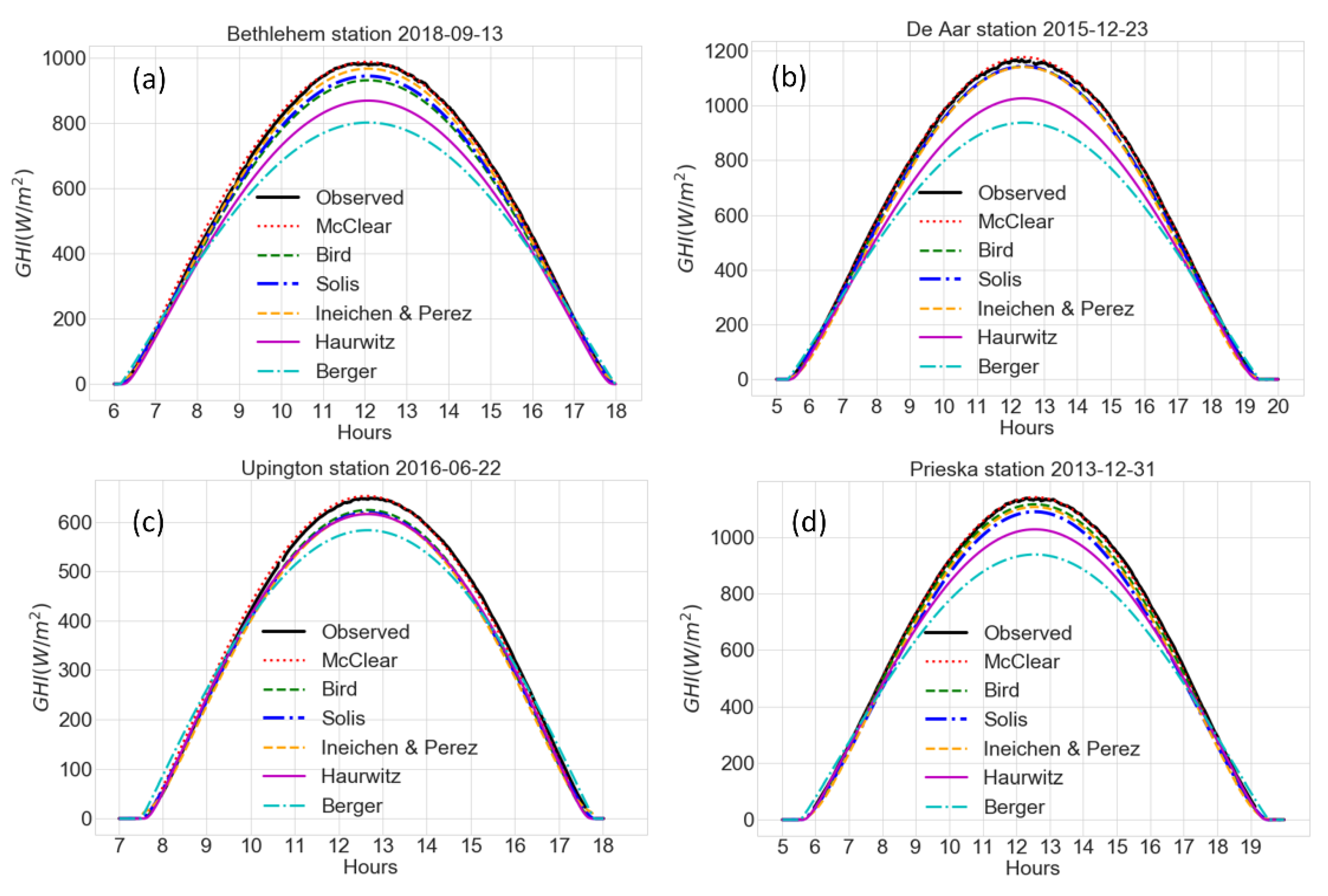
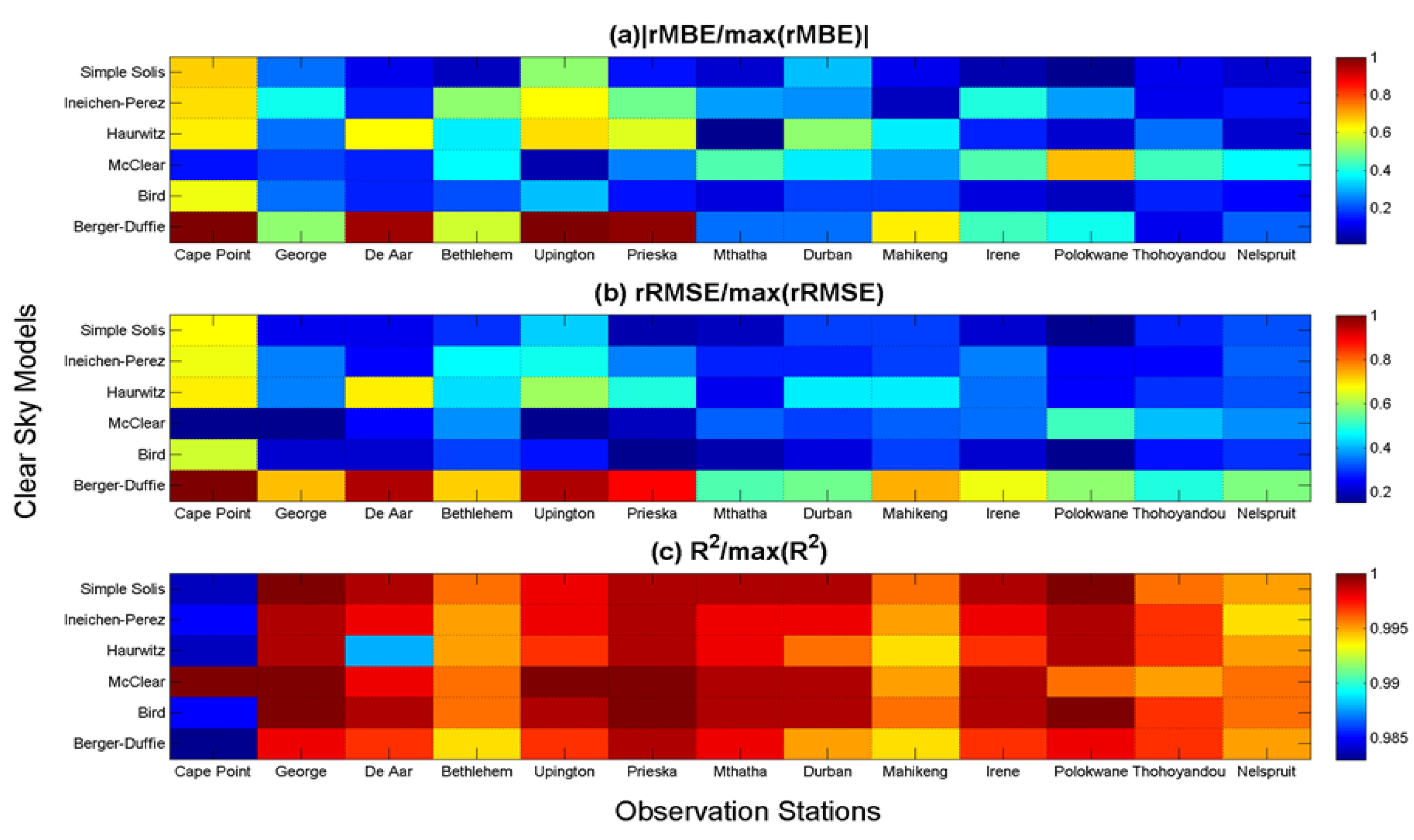
4.2. Validation Results

After detecting clear sky times, a random set of days for each of the 13 stations is shown in Figure 6, Figure 7 and Figure 8. All the models generated data that captured temporal variability but with varying accuracy. The full assessment of each model’s performance per site is given by the statistics in Supplementary Tables S1–S6. Additionally, colormaps are provided in Figure 9 and Figure 10 for the comparison of model performance per station and climate region. A summary of performance is given in

Table 3. Optimum model w.r.t metrics for each station.

Station	Minimum rMBE	Minimum rRMSE	Maximum R2
Cape Point	Berger-Duffie	McClear	McClear
George	McClear	McClear	Bird
De Aar	Simple Solis	Bird	Bird
Bethlehem	Simple Solis	Simple Solis	Bird
Upington	McClear	McClear	McClear
Prieska	Bird	Bird	Bird
Mthatha	Haurwitz	Bird	Bird
Durban	Bird	Bird	Bird
Mahikeng	Ineichen-Perez	Ineichen-Perez	McClear
Irene	Simple Solis	Simple Solis	Bird
Polokwane	Simple Solis	Bird	Bird
Thohoyandou	Ineichen-Perez	Ineichen-Perez	McClear
Nelspruit	Simple Solis	Bird	Bird

and

Table 4. Indication of number of stations with an optimum metric.

Clear Sky Model	Number of Stations with Minimum rMBE	Number of Stations with Minimum rRMSE	Number of Stations with Maximum R2
Berger-Duffie	1	0	0
Bird	2	6	9
McClear	2	3	4
Haurwitz	1	0	0
Ineichen-Perez	2	2	0
Simple Solis	5	2	0

. Table 3 shows the optimum model w.r.t metrics for each station, whilst Table 4 shows the number of stations where a model shows an optimum metric. An optimum model per metric and station is found as follows: minimum $rMBE$, minimum $rRMSE$ and maximum ${\mathrm{R}}^2$. Further, scatter plots are presented in the study to show the correlation between measured and modelled clear sky GHI for each model and per station.

4.3. Validation and Comparison of the Results with Other Literature

From Table S1 and Figure 9c, the Bird model had excellent performance, with an rRMSE of less than 5% at all of the stations except for Bethlehem, Mahikeng, and Cape Point, and good performance in Bethlehem and Mahikeng (with $5\%\le rRMSE<10\%$). This clear sky model also has acceptable performance at the Cape Town station, with respect to rRMSE (with $10\%\le rRMSE<15\%$). Overall, with just the rRMSE in analysis, the Bird model did not show poor performance at any of the stations. The performance of the Bird model is also verified in Table 4, where the model is observed to have the minimum rRMSE at six (46%) of the stations when compared to the rRMSE of the other five models. The McClear model performed optimally, w.r.t. a minimum rRMSE, at three stations, and the Ineichen–Perez and Simple Solis both have optimal performance at two stations. In considering the correlation coefficient, the Bird model has optimal performance, w.r.t. a maximum R², at nine of the stations and the McClear model showed optimal performance at the remaining four stations.

Generally, the presented results for the Bird model at the six stations are comparable and even better than other literature studies which lie in the same latitudes as the South Africa stations. Some of the literature results are given in the shaded block in Table S5. The better results might be because of using monthly satellite albedo instead of a default value, calculating $P_w$ from measured temperature and humidity instead of climatologies, and using actual station pressure. $O_3$ was the only input that was sourced as monthly climatology values from SoDa [39]. According to Bird et al., 1981 [17], $O_3$ has a minor effect on irradiance, and Polo et al. [1] reported that the variability of daily $O_3$ ozone is low. The good performance of the Bird model in the study might be as a result of using high spatio-temporal atmospheric input parameters. As shown in Figure 9a, in considering the rMBE recorded with the Bird model, this model did underestimate GHI at all stations except for Thohoyandou, where the model overestimated the irradiance.

From Table S2 and Figure 9c, the McClear clear sky model had excellent performance in five stations: Upington, De Aar, Prieska, George and Cape Point with rRMSE < 5%, and good performance in the rest of the stations (with $5\%\le rRMSE<10\%$). The rMBE polarity in Figure 9a shows that the McClear model overestimated GHI in 10 of the 13 stations, with underestimations at Thohoyandou, Polokwane and Cape Point, which are locations in the “extreme” latitudes for the study region. Overall, the McClear model was outperformed by Simple Solis and Bird in South African locations. This may mean that the “black box” model needs further improvement to be able to estimate irradiance with better accuracy in South African locations. Still, the McClear model performs well and it has an advantage over all the other models because the data are readily available and there is no need to configure and provide input parameters.

From Table S3 and Figure 9c, the Simple Solis clear sky model had excellent performance in Thohoyandou, Polokwane, Bethlehem, Irene, Prieska, De Aar, Mthatha and George with rRMSE < 5%. The model had good performance in Nelspruit, Mahikeng, Upington, Durban and Cape Point with $AO{D}_{550}$. As shown by the rMBE polarity in Figure 9a, the Simple Solis model overestimated GHI in 3 of the 13 stations, namely Thohoyandou, Polokwane and Irene. The results for Simple Solis performance are comparable and even better than other literature studies which lie in the same latitudes as South Africa. The better results might be because of using high spatiotemporal resolution model inputs, using actual station pressure, daily $AO{D}_{1240}$ from SoDa [39] and $P_w$ calculated from measured temperature and humidity.

From Table S4 and Figure 9c, the Ineichen–Perez clear sky model had excellent performance in Thohoyandou, Polokwane, Durban, De Aar and Mthatha with rRMSE < 5%. The model had good performance for the rest of the stations with $5\%\le rRMSE<10\%$. The model underestimated GHI in 6 out of 13 stations, as shown in the rMBE polarity in Figure 9a. The model performed less fairly, with an overall rRMSE of 5.74%, when compared against other complex models—rRMSE of 4.11% for Bird, 4.61% for Simple Solis and 5.06% for McClear. This might be because Ineichen–Perez is the only model that depends on TL as an input. The TL data were sourced as monthly climatologies from SoDa [39]. According to Ineichen (2006) [16], TL has the highest influence on model accuracy. The model accuracy might improve with locally measured TL, though TL observations were not available in the area of study.

From Table S5 and Figure 9c, the Haurwitz clear sky model performed excellently in Polokwane and Mthatha with rRMSE < 5%. The model had good performance at the other stations but average performance, i.e., rRMSE >10%, in Upington and De Aar, which are stations that receive very high irradiance. The model underestimated irradiance at all the stations except in Thohoyandou, Nelspruit and Durban, as shown by rMBE polarity in Figure 8a. The performance of the model may be a result of the calibration of the Haurwitz model. The Blue Hill observatory where the coefficients a and b were calibrated has different atmospheric constituents to South African locations. There is a need to calibrate coefficients a and b using data measured from South African locations.

From Table S6 and Figure 9c, the Berger–Duffie clear sky model did not have excellent performance in any of the locations. No station had rRMSE < 5%. The model had good performances in Thohoyandou, Nelspruit, Mthatha and Durban, with $5\%\le rRMSE<10\%$, but average performance in Polokwane, Bethlehem, Mahikeng, Irene, and George—with $10\%\le rRMSE<15\%$. The model had poor performance in areas that receive very high irradiance, namely Upington, De Aar and Prieska. The model underestimated irradiance in almost all the sites except in Durban, as shown by rMBE polarity in Figure 9a. From the results, since the transmittance of the model was integrated to a constant of 0.7, there is a need to recalibrate the constant for each of the South African sites.

The plots in Figure 10a–c show the stations grouped within climate zones, and the data are presented with metrics normalised relative to the optimum value across all models and all stations, for each metric. Table 4 shows the resulting optimum model at each station and within the climate belts. Both Cape Point and George are in the temperate coastal belt, and Figure 10a–c and Table 4 show that the McClear model is the best performing for this temperate coastal belt. On the other hand, for the cold interior stations, namely De Aar and Bethlehem, the model with optimal results is either Bird or Simple Solis. For the arid interior region (with Upington and Prieska), either the McClear or Bird model is optimal. The Bird model is the most likely model for the subtropical coastal belt, with Mthatha and Durban. For the temperate interior—with Mahikeng, Irene and Polokwane—no clear optimal model can be picked out from Table 4, but visual inspection of Figure 10a–c suggests that the most feasible model is either Simple Solis or Bird. There is no clear optimal model for the stations Thohoyandou and Nelspruit, which are both in the hot interior region.

From Tables S1–S5, the model performances based on the overall rRMSE were as follows: Bird 4.11%, Simple Solis 4.61%, McClear 5.06%, Ineichen–Perez 5.74%, Haurwitz 7.04% and Berger–Duffie 12.17%. The overall rMBE was positive for McClear + 1.39%, meaning that the model overestimates GHI. The correlation between measured clear sky GHI and corresponding modelled GHI results and a brief description are given in the (Supplementary Materials Figures S1–S13), and the 1:1 (black dotted) line explains the correlation—the closer the values to the line, the better the model, and vice versa. The correlation results agreed with the statistics from Tables S1–S5.

5. Conclusions

In this study, the performance of six GHI clear sky models, namely Bird, Simple Solis, McClear, Ineichen–Perez, Haurwitz and Berger–Duffie, have been evaluated against reference Baseline Solar Radiation Network quality guided 1-min data for 13 stations in the South African Weather Services radiometric network. The stations are located in six climatological regions. All the models assessed were capable of reproducing GHI irradiance, but with different accuracy in different stations. All four complex models, namely Bird, Simple Solis, McClear and Ineichen–Perez, performed well with rRMSE less than 10% in all the stations. The simple models, Haurwitz and Berger–Duffie, did not perform well overall in South African locations. Bird was the overall best model, followed by Simple Solis, McClear, Ineichen–Perez, Haurwitz and Berger–Duffie. The McClear model overestimated GHI and the other five models underestimated GHI. Model inputs seem to influence the model performance. There is also an indication that each model behaves differently over particular climate regions.

Future studies will focus on validating more clear sky GHI models and other solar radiation parameters and optimising or calibrating simple models’ coefficients for each site. Future work will also focus on sourcing high temporal and spatial resolution model inputs from different databases and trying to re-validate models to find suitable model inputs. Future studies will also focus on using the results for renewable energy applications.

The challenge encountered in the study was the absence of high temporal and spatial resolution model inputs. It is recommended that GHI monitoring stations also measure high temporal and high spatial resolution water vapour, aerosols, ozone and albedo to aid model assessment studies. Some other researchers who may want to replicate the study in their countries or regions might not have reference measured GHI data and atmospheric model input parameters to assess and validate the clear sky models in their regions.

References

1. Polo, J.; Martín-Pomares, L.; Gueymard, C.A.; Balenzategui, J.L.; Fabero, F.; Silva, J.P. Fundamentals: Quantities, Definitions, and Units. In Solar Resource Mapping—Fundamentals and Applications; Green Energy and Technology; Polo, J., Martín-Pomares, L., Sanfilippo, A., Eds.; Springer: Zurich, Switzerland, 2019; pp. 1–14. [Google Scholar] [CrossRef]
2. Reno, M.J.; Hansen, C.W.; Stein, J.S. Global Horizontal Irradiance Clear Sky Models: Implementation and Analysis; SAND2012-2389; Sandia National Laboratories: Albuquerque, NM, USA; Livermore, CA, USA, 2012; Available online: https://scholar.google.com/scholar?q=related:NRwgbk5tC6sJ:scholar.google.com/&scioq=&hl=en&as_sdt=0,5 (accessed on 23 June 2020).
3. Gairaa, K.; Benkaciali, S.; Guermoui, M. Clear-sky models evaluation of two sites over Algeria for PV forecasting purpose. Eur. Phys. J. Plus 2019, 134, 534. [Google Scholar] [CrossRef]
4. Sun, X.; Bright, J.M.; Gueymard, C.A.; Acord, B.; Wang, P.; Engerer, N.A. Worldwide performance assessment of 75 global clear sky irradiance models using Principal Component Analysis. Renew. Sustain. Energy Rev. 2019, 111, 550–570. [Google Scholar] [CrossRef]
5. Engerer, N.A.; Mills, F.P. Validating nine clear sky radiation models in Australia. Sol. Energy 2015, 120, 9–24. [Google Scholar] [CrossRef]
6. Dazhia, Y.; Jirutitijaroena, P.; Walshb, W.M. The Estimation of Clear Sky Global Horizontal Irradiance at the Equator. Energy Procedia 2012, 25, 141–148. [Google Scholar] [CrossRef] [Green Version]
7. Antonanzas-Torres, F.; Urraca, R.; Polo, J.; Perpiñán-Lamigueiro, O.; Escobar, R. Clear sky solar irradiance models: A review of seventy models. Renew. Sustain. Energy Rev. 2019, 107, 374–387. [Google Scholar] [CrossRef]
8. Badescu, V.; Gueymard, C.A.; Cheval, S.; Oprea, C.; Baciu, M.; Dumitrescu, A.; Iacobescu, F.; Milos, I.; Rada, C. Accuracy analysis for fifty-four clear-sky solar radiation models using routine hourly global irradiance measurements in Romania. Renew. Energy 2013, 55, 85–103. [Google Scholar] [CrossRef]
9. Mikofski, M.M.; Hansen, C.W.; Holmgren, W.F.; Kimbal, G.M. Use of measured aerosol optical depth and precipitable water to model clear sky irradiance. In Proceedings of the 2017 IEEE 44th Photovoltaic Specialist Conference (PVSC), Washington, DC, USA, 25–30 June 2017; pp. 110–116. Available online: https://ieeexplore.ieee.org/abstract/document/8366314 (accessed on 15 June 2020).
10. Laguarda, A.; Abal, G. Clear-sky broadband irradiance: First model assessment in Uruguay. In Proceedings of the Publicado en las Actas del ISES Solar World Congress, Abu Dabi, United Arab Emirates, 10 July 2017; Available online: https://www.colibri.udelar.edu.uy/jspui/handle/20.500.12008/21620?mode=full (accessed on 16 September 2020). [CrossRef]
11. Fourie, C.H.; Winkler, H.; Roro, K. Modelling atmospheric radiative transfer conditions and its comparison to empirical solar irradiance in South Africa. In Proceedings of the South African Solar Energy Conference (SASEC), Mpekweni Beach Resort, Eastern Cape Province, South Africa, 25–27 November 2019; Available online: https://www.sasec.org.za/papers2019/7.pdf (accessed on 25 February 2020).
12. Martín-Pomares, L.; Romeo, M.G.; Polo, J.; Frías-Paredes, L.; Fernández-Peruchena, C. Sampling Design Optimization of Ground Radiometric Stations. In Solar Resources Mapping. Green Energy and Technology; Springer: Cham, Switzerland, 2019; pp. 253–281. [Google Scholar] [CrossRef]
13. Masoom, A.; Kashap, Y.; Bansal, A. Solar Radiation Assessemnt and Forecasting Using Satellite Data; Tyagi, H., Agarwal, A.K., Chakraborty, P.R., Powar, S., Eds.; Springer: Singapore, 2019; pp. 45–71. [Google Scholar] [CrossRef]
14. Dev, S.; Manandhar, S.; Lee, Y.H.; Winkler, S. Study of clear sky models for Singapore. In Progress in Electromagnetics Research Symposium-Fall (PIERS-FALL); Singapore. 2017, pp. 1418–1420. Available online: https://ieeexplore.ieee.org/abstract/document/8293352 (accessed on 1 November 2020).
15. Lefèvre, M.; Oumbe, A.; Blanc, P.; Espinar, B.; Gschwind, B.; Qu, Z.; Wald, L.; Schroedter-Homscheidt, M.; Hoyer-Klick, C.; Arola, A.; et al. Mcclear: A new model estimating downwelling solar radiation at ground level in clear-sky conditions. Atmos. Meas. Tech. 2013, 6, 2403–2418. Available online: www.atmos-meas-tech.net/6/2403/2013/doi:10.5194/amt-6-2403-2013 (accessed on 14 July 2020). [CrossRef] [Green Version]
16. Ineichen, P. Comparison of eight clear sky broadband models against 16 independent data banks. Sol. Energy 2006, 80, 468–478. [Google Scholar] [CrossRef] [Green Version]
17. Bird, R.E.; Hulstrom, R.L. Simplified Clear Sky Model for Direct and Diffuse Insolation on Horizontal Surfaces; No. SERI/TR-642-761; Solar Energy Research Inst.: Golden, CO, USA, 1981. [Google Scholar]
18. Daryl, R.M. Solar Radiation, Practical Modeling for Renewable Energy Applications. Energy and the Environment; CRC Press: Boca Raton, FL, USA, 2013. [Google Scholar]
19. Hersbach, H.; Bell, B.; Berrisford, P.; Biavati, G.; Horányi, A.; Muñoz Sabater, J.; Nicolas, J.; Peubey, C.; Radu, R.; Rozum, I.; et al. The ERA5 Global Reanalysis. Q. J. R. Meteor. Soc. 2020, 146, 1999–2049. [Google Scholar] [CrossRef]
20. Reno, M.J.; Hansen, C.W. Identification of periods of clear sky irradiance in time series of GHI measurements. Renew. Energy 2016, 90, 520–531. [Google Scholar] [CrossRef] [Green Version]
21. Zhandire, E. Predicting clear-sky global horizontal irradiance at eight locations in South Africa using four models. J. Energy S. Afr. 2017, 28, 77–86. [Google Scholar] [CrossRef]
22. Patel, S.S.; Rix, A.J. Water surface albedo modelling for floating photovoltaic plants. In Proceedings of the South African Solar Energy Conference (SASEC), Mpekweni Beach Resort, Eastern Cape Province, South Africa, 25–27 November 2019; Available online: https://www.sasec.org.za/papers2019/8.pdf (accessed on 27 February 2020).
23. Javu, L.; Winkler, H.; Roro, K. Validating clear-sky irradiance models in five South African locations. In Proceedings of the South African Solar Energy Conference (SASEC), Mpekweni Beach Resort, Eastern Cape Province, South Africa, 25–27 November 2019; Available online: https://www.sasec.org.za/papers2019/6.pdf (accessed on 15 February 2020).
24. Mueller, R.; Dagestad, K.; Ineichen, P.; Schroedter-Homscheidt, M.; Cros, S.; Dumortier, D.; Kuhlemann, R.; Olseth, J.; Piernavieja, G.; Resie, C.; et al. Rethinking satellite based solar irradiance modelling. The SOLIS clear-sky module. Remote Sens. Environ. 2004, 91, 160–174. Available online: https://www.sciencedirect.com/science/article/abs/pii/S0034425704000690 (accessed on 27 September 2020). [CrossRef]
25. Ineichen, P. A broadband simplified version of the Solis clear sky model. Sol. Energy 2008, 82, 758–762. [Google Scholar] [CrossRef] [Green Version]
26. Ineichen, P.; Perez, R. A new airmass independent formulation for the Linke turbidity coefficient. Sol. Energy 2002, 73, 151–157. [Google Scholar] [CrossRef] [Green Version]
27. Perez, R.; Ineichen, P.; Moore, K.; Kmiecik, M.; George, R.; Vignola, F. A new operational model for satellite-derived irradiances: Description and validation. Sol. Energy 2002, 73, 307–317. [Google Scholar] [CrossRef] [Green Version]
28. Haurwitz, B. Insolation in relation to cloudiness and cloud density. J. Meteorol. 1945, 2, 154–166. [Google Scholar] [CrossRef]
29. Haurwitz, B. Isolation in relation to cloud type. J. Meteorol. 1948, 5, 110–113. [Google Scholar] [CrossRef] [Green Version]
30. Berger, X. Etude du Climat en Region Nicoise en vue d’Applications a l’Habitat Solaire; CNRS: Paris, France, 1979. [Google Scholar]
31. Solar Radiation Data (SoDa) Service. Available online: http://www.soda-pro.com/web-services (accessed on 2 March 2020).
32. Copernicus Portal. Available online: https://atmosphere.copernicus.eu/data (accessed on 16 March 2020).
33. Gschwind, B.; Wald, L.; Blanc, P.; Lefèvre, M.; Schroedter-Homscheidt, M.; Arola, A. Improving the McClear model estimating the downwelling solar radiation at ground level in cloud-free conditions–McClear-v3. Meteorol. Z. 2019, 28, 147–163. [Google Scholar] [CrossRef]
34. Ineichen, P. Quatre Années de Mesures D’ensoleillement à Genève. Ph.D. Thesis, University of Geneva, Geneva, Switzerland, 1983. [Google Scholar] [CrossRef]
35. Kasten, F. Parametrisierung der Globalstrahlung durch Bedeckungsgrad und Truebungsfaktor. In Proceedings of the Deutsche Meteorologen-Tagung 1983, Bad Kissingen, Germany, 16–19 May 1983; pp. 49–50. Available online: https://ci.nii.ac.jp/naid/10021899342/ (accessed on 11 June 2020).
36. Mabasa, B.; Lysko, M.D.; Tazvinga, H.; Mulaudzi, S.T.; Zwane, N.; Moloi, S.J. The Ångström–Prescott Regression Coefficients for Six Climatic Zones in South Africa. Energies 2020, 13, 5418. [Google Scholar] [CrossRef]
37. Karlsson, K.; Anttila, K.; Trentmann, J.; Stengel, M.; Meirink, J.F.; Devasthale, A.; Hanschmann, T.; Kothe, S.; Jääskeläinen, E.; Sedlar, J.; et al. CLARA-A2.1: CM SAF cLoud, Albedo and Surface RAdiation Dataset from AVHRR Data—Edition 2.1; Satellite Application Facility on Climate Monitoring (CM-SAF): Offenbach, Germany, 2020. [Google Scholar] [CrossRef]
38. Frederick, J.E. Ozone Depletion and Related Topic, Ozone as a UV Filter; Elsevier: Amsterdam, The Netherlands, 2015; pp. 359–363. [Google Scholar]
39. SODA Portal. Available online: http://www.soda-pro.com/web-services/atmosphere/linke-turbidity-factor-ozone-water-vapor-and-angstroembeta (accessed on 21 April 2020).
40. Diabate, L.; Remund, J.; Wald, L. Linke turbidity factors for several sites in Africa. Sol. Energy 2003, 75, 111–119. [Google Scholar] [CrossRef] [Green Version]
41. SODA Portal. Available online: http://www.soda-pro.com/web-services/atmosphere/cams-aod (accessed on 21 February 2020).
42. Ångström, A. On the Atmospheric Transmission of Sun Radiation and on Dust in the Air. Geogr. Ann. 1929, 11, 156–166. [Google Scholar] [CrossRef]
43. Ångström, A. Techniques of Determinig the Turbidity of the Atmosphere. Tellus 1961, 13, 214–223. [Google Scholar] [CrossRef] [Green Version]
44. Keogh, W.M.; Blakers, A.W. Accurate measurement, using natural sunlight, of silicon solar cells. Prog. Photovolt. Res. Appl. 2004, 12, 1–19. [Google Scholar] [CrossRef]
45. Gueymard, C. Analysis of monthly average atmospheric precipitable water and turbidity in Canada and northern United States. Sol. Energy 1994, 53, 57–71. [Google Scholar] [CrossRef]
46. Gueymard, C. Assessment of the accuracy and computing speed of simplified saturation vapour equations using a new ref-erence dataset. J. Appl. Meteorol. 1993, 32, 1294–1300. [Google Scholar] [CrossRef] [Green Version]
47. Reda, I.; Andreas, A. Solar position algorithm for solar radiation applications. Sol. Energy 2004, 76, 577–589. [Google Scholar] [CrossRef]
48. Holmgren, W.F.; Hansen, C.; Mikofski, M. Pvlib python: A python package for modeling solar energy systems. J. Open Source Softw. 2018, 3, 884. [Google Scholar] [CrossRef] [Green Version]
49. Iqbal, M. An Introduction to Solar Radiation; Academic Press: Toronto, ON, Canada, 1983. [Google Scholar]
50. Duffie, J.A.; Beckman, W.A. Solar Engineering of Thermal Processes; John Wiley & Sons, Inc.: Hoboken, NJ, USA, 1980; pp. 6–13. [Google Scholar]
51. Cooper, P.I. The absorption of radiation in solar stills. Sol. Energy 1961, 12, 333–346. [Google Scholar] [CrossRef]
52. Spencer, J.W. Fourier series reprensentation of the position of the sun. Search 1971, 2, 172. Available online: https://ci.nii.ac.jp/naid/10005108360/ (accessed on 2 April 2020).
53. Kasten, F.; Young, A.T. Revised optical air mass tables and approximation formula. Appl. Opt. 1989, 28, 4735–4738. [Google Scholar] [CrossRef]
54. Gueymard, C.A. The sun’s total and spectral irradiance for solar energy applications and solar radiation models. Sol. Energy 2004, 76, 423–453. [Google Scholar] [CrossRef]
55. Long, C.N.; Dutton, E.G. BSRN Global Network Recommended QC Tests, V2. 2010. Available online: https://epic.awi.de/30083/1/BSRN_recommended_QC_tests_V2.pdf (accessed on 11 December 2019).
56. Driemel, A.; Augustine, J.; Behrens, K.; Colle, S.; Cox, C.; Cuevas-Agulló, E.; Denn, F.M.; Duprat, T.; Fukuda, M.; Grobe, H.; et al. Baseline Surface Radiation Network (BSRN): Structure and data description (1992–2017). Earth Syst. Sci. Data 2018, 10, 1491–1501. [Google Scholar] [CrossRef] [Green Version]
57. Maupin, K.A.; Swiler, L.P.; Porter, N.W. Validation Metrics for Deterministic and Probabilistic Data. J. Verificat. Valid. Uncertain. Quantif. 2018, 3, 031002. [Google Scholar] [CrossRef]
58. Long, C.; Shi, Y. An automated quality assessment and control algorithm for surface radiation measurements. Open Atmos. Sci. J. 2008, 2, 23–37. Available online: https://openatmosphericsciencejournal.com/VOLUME/2/PAGE/23/FULLTEXT/ (accessed on 15 February 2020). [CrossRef] [Green Version]
Figure 1. A map showing South African Weather Service’s radiometric station location and climatic zones (Adapted from Mabasa et al., 2020 [57]).
Energies 14 02583 g001
Figure 2. The flowchart of the approach summarising the methodology from clear sky detection to model classification based on their performance. {Fifth generation European Centre for Medium-Range Weather Forecasts atmospheric reanalysis (ERA5); Global horizontal irradiance (GHI); Quality control (QC); Baseline Surface Radiation Network (BSRN)}.
Energies 14 02583 g002
Figure 3. A plot of observed radiation data on 11 November 2014 at Upington station (a), and De Aar station (b), 6 clear models and extra-terrestrial radiation on a horizontal surface on what ERA5 data classified as a cloudy day.
Energies 14 02583 g003
Figure 4. Illustration of Reno and Hansen methodology (a) Predicted irradiances with the 6 models and George station observed radiation on 29 January 2016 after only applying ERA5 reanalysis data set, (b) McClear and observed irradiance, (c) observed radiation after Reno and Hansen method is applied to detect not clear periods, (d) complete clear sky observed radiation and 6 clear sky models.
Energies 14 02583 g004
Figure 5. A plot of observed radiation data on 29 January 2016 from 08:30 am to 09:00 am at George station and McClear model on a corresponding period (a) and a plot of observed radiation data and 6 clear sky models on the corresponding period (b).
Energies 14 02583 g005
Figure 6. Comparison between observed and modelled minute GHI values in Bethlehem (a), De Aar (b), Upington (c), and Prieska (d).
Energies 14 02583 g006
Figure 7. Comparison between observed and modelled minute GHI values in Mahikeng (a), Irene (b), Polokwane (c), and Thohoyandou (d).
Energies 14 02583 g007
Figure 8. Comparison between observed and modelled minute GHI values in Cape Point (a), Nelspruit (b), Durban (c), and Mthatha (d).
Energies 14 02583 g008
Figure 9. Overall performance of the six models at the 13 stations.
Energies 14 02583 g009
Figure 10. Stations grouped within climate zones with metrics normalised relative to the optimum value across all models and all stations, for each metric.
Energies 14 02583 g010