Abstract
The green energy transition is associated with the use of a wide range of metals and minerals that are exhaustible. Most of these minerals are limited in access due to small resource fields, their concentration in several locations and a broader scale of industry usage which is not limited exclusively to energy and environmental sectors. This article classifies 17 minerals that are critical in the green energy transition concerning the 10 main technologies. The following classification signs of metal resources were used: (1) the absolute amount of metals used in the current period for energy; (2) projected annual demand in 2050 from energy technologies as a percentage of the current rate; (3) the number of technologies where there is a need for an individual metal; (4) cumulative emissions of CO2, which are associated with metal production; (5) period of reserves availability; (6) the number of countries that produced more than 1% of global production; (7) countries with the maximum annual metal productivity. The ranking of metals according to these characteristics was carried out using two scenarios, and the index of the availability of each mineral was determined. The lowest availability index values (up to 0.15) were calculated for cobalt, graphite and lithium, which are key battery minerals for energy storage. Low indices (up to 0.20) were also obtained for iron, nickel and chromium. The calculation of the availability index for each mineral was enhanced with linear trend modelling and the fuzzy logic technique. There are two scenarios of demand–supply commodity systems with a pre-developed forecast up to 2050: basic independent parameter probability and balanced fuzzy sum. Both scenarios showed comparable results, but the second one highlighted supply chain importance. Generally, the lowest availability index values (up to 0.15) were calculated for cobalt, graphite and lithium, which are key battery minerals for energy storage. Low indices (up to 0.20) were also obtained for iron, nickel and chromium. The fuzzy logic model helped to reveal two scenarios up to 2050. The two scenarios presented in the current research expose a high level of uncertainty of the projected 2050 forecast.
1. Introduction
The green energy transition is associated with the use of a wide range of metals and minerals that are exhaustible [1]. Many enthusiastic policy makers and scientists believe hypotheses that are not possible concerning the physics of the fuel society. The reason for this is the shortage of resources, once again. No energy system, in short, is actually “renewable”, since all machines require the continual mining and processing of millions of tons of primary materials and the disposal of hardware that inevitably wears out [2]. Most of these minerals are limited in access due to resource fields that are small in nature, their concentration in several locations and a huge scale of industry usage not only in energy and environmental restrictions. To form an objective mineral policy [3,4], countries need to understand the place and characteristics of each mineral in the resource base (both at a global and regional scale).
Renewable energy sources are mostly unlimited resources, in the human dimension. The main factor holding back a large-scale move away from fossil oil and gas was the lack of efficient and inexpensive energy storage. However, the global green energy transition has begun and is underway, and the main forecast figures were calculated for the period up to 2050. This is in line with the forecasts of the World Bank for Estimating Demand of Minerals for 2050 Energy Technology Scenarios [5]. The limited and most valuable resources have become “battery metals”, which are necessary for the production of energy storage, regardless of the source itself.
The World Bank forecasts [6] the production of battery metals, such as graphite, lithium and cobalt, to grow by almost 500% by 2050 to meet the growing demand for clean energy technologies. The growth in demand for metals until 2050 will amount to Li: 965%; Co: 585%; Ni: 108%; and graphite: 383%. A list of critical minerals that are required for green energy transition includes aluminium, chromium, cobalt, copper, graphite, indium, iron, lead, lithium, manganese, molybdenum, neodymium, nickel, silver, titanium, vanadium and zinc. Most of these metals are critical minerals for developed countries. Critical minerals are considered vital to the world’s largest economies, but whose supply is at risk due to geological resource deficit, geopolitical issues, trade policies or other external factors. Limited access to the resources, a large-scale expansion in their use and geopolitical risks in their supply form the need for manufacturers to have are source base. This primary link already determines production risks, and in the future, the resource base is considered as the most deficient and strategic component of energy production.
All these minerals and metals are exhaustible and non-renewable resources. The best resources are rapidly depleting against the background of consumption intensity. These processes begin with a deterioration in the mining conditions of existing deposits and a shortage of high-quality raw materials. This is how more complex deposits and less concentrated ores are used, which leads to a significant increase in the cost of metals. The metals resources cannot be physically increased, and this irreversibly leads to an increase in the cost of the resource. With each year of growth in consumption and decrease in resources, the price of the metals grows exponentially (Appendix A and Appendix B).
The main risks of real production in most developed countries are associated with the distribution of reserves and mining enterprises. The Asia-Pacific region has dominated the battery metals market and accounts for up to 90% of its value. This regional trend is expected to continue for several decades. This enables producer countries to use the availability of resources as a strong geopolitical tool. It should be noted that China is the leader in greenhouse gas emissions, and a significant part of the total emissions depends on mining and metal production [7,8]. This factor can aggravate not only the risks of green energy production but also delay the goals of that transition.
Over the past decade, China has cut off the supply of critical minerals twice, such as rare earth and its concentrates, to Japan and the United States, which served to exacerbate long-term raw material wars. Such conflicts cannot be resolved in the short term, since deposit development is a very difficult capital-intensive process, and it requires many years to complete.
To implement a green energy transition, countries need to model several options for the supply of critical metals. For such modelling, the available metal reserves were classified taking into account the following factors: (1) the absolute amount of metals used in the current period for energy; (2) projected annual demand for 2050 from energy technologies as a percentage of the current rate; (3) the number of technologies where there is a need for an individual metal; (4) cumulative CO2 emissions which are associated with metal production; (5) the period of reserves availability; (6) the number of countries that produced more than 1%of global production; (7) countries with the maximum annual metal productivity. The ranking of metals according to these characteristics was carried out, and the index of the availability of each mineral was determined. The article classified 17 minerals that are critical in the green energy transition concerning the 10main technologies—Wind, solar photovoltaic, concentrated solar power, hydro, geothermal, energy storage, nuclear, coal, gas, carbon capture and storage. The metals and minerals that are taken into account are all ferrous and non-ferrous metals, minor metals, rare earth metals (neodymium) and graphite. A separate indicator takes into account the use of metal in the listed green energy technologies. Some metals are critical, but only for one technology (graphite in batteries and neodymium in wind turbines), but copper, which is used in all the listed technologies and industries, is a critical element for realizing a low-carbon future.
The aim of this article is the definition and scoring of availability indices for critical metals that are used in the energy sector. Their availability will determine the implementation of the green energy transition as a whole and the implementation of individual technologies. The novelty of the approach lies in the method to determine the availability of strategic and critical types of mineral raw materials on which the green energy transition is based. For EU countries, the USA and Canada, these tools are known and traditional, but for many countries, these methods have not been developed, although there is a need for a normative definition of critical metals. For example, in Ukraine, the concepts of “strategic”, “critical” minerals have been introduced normatively, but the methodology for their calculation has not yet been determined. For each region and country, this approach can be complemented by regional criteria of importance.
Existing methodologies for assessing resource depletion are based on a quantitative comparison of mineral reserves and the existing rate of their extraction. Very often, existing models of depletion resources do not take into account the political, organizational and other risks of accessibility. Determining critical minerals most often involves the use intensity indicators in domestic production, the availability of own resources and rate of import dependence. Thus, these approaches consider only the past or current situation, not assuming the future impact of mineral consumption and its possible harmful effect mitigation. The calculations given in the article relate not only to today’s but also to future indicators of metal consumption. Many external risks are also included in the consideration. In an additional scenario, the compromise approach between data-driven and expert-driven estimation was realized. The impact of different indices was grouped by risk types—Supply risk, demand risk and geopolitics risk. To estimate the integral probability of success of such demand–supply system, we used a fuzzy logic model.
Additionally, a remarkable feature of the author’s approach is the use of resource data that are aggregated by the USGS, since most of the reports on resource depletion use separate national data. Such data are collected in each region using quite different accounting systems. Aggregated data make it possible to take into account possible differences in the national definition and classification of available resources. The novelty of the approach is enhanced by the application of powerful forecasting methods, such as the trend modelling and fuzzy logic models.
The logic of the research influences the structure of the presented paper so that the introduction sheds light on the problem’s actuality and the necessity to research it; then, there is evidence of the research gap and scholars’ attempts to reveal the possible decision of the considered scientific problem in the literature review. The methodology and data are presented in the next part, which is followed with its implementation accomplished with the forecasting of possible results. Conclusions and the discussion of research milestones and possible policy recommendations conclude the paper.
2. Literature Review
The mobilisation of the industry for a clean and circular economy (CE) became the central point for The European Green Deal of the EU. The new strategy for economic growth adopted by the EU in late 2019 pushed the transition towards a CE model, which was announced in 2014 [9]. The CE assumes a transition from a linear model based on take–make–dispose to a circular model [10]. The key policy recommendations within the framework of limited critical resources and a green energy transition found their place as the object of the contemporary research literature:
- (1)
- Identify differences in technologies with respect to size, component configuration, chemistry, material composition and other factors that might impact the energy, environmental and cost impacts of recycling these materials (i.e., [11]);
- (2)
- Identify current and near-term (5–10 years) future commercial processes being used or that could be used for the recycling and reuse of these material-based products at their end-of-useful life (i.e., [12]);
- (3)
- Identify the potential technical, environmental, cost and energy impacts associated with the recycling of these materials and second-life applications, including any engineering or financial obstacles or other barriers (i.e., [13,14,15];
- (4)
- Identify knowledge gaps and areas that could be further investigated (i.e., [16]);
- (5)
- Document the study findings in a clearly laid out and easy-to-follow report clearly fulfilling the key “refurbish, reuse, recycle” circular economy principle (i.e., [17]).
Note, a number of new mineral recycling technologies currently in development attempt to increase the recovery rate for various metals, such as cobalt and nickel, through the recycling system. These technologies focus on hydrometallurgical processes, which are less energy intensive than pyrometallurgical processes. The new recycling technologies commit to increasing recycling rates to a reported 90%+. The companies developing these new recycling technologies are most interested in direct recycling or cathode-to-cathode recycling to recover chemicals and chemical powders suitable for direct sale back to initial product manufacturers. However, none of these technologies are yet operating at scale, which is the current challenge [18].
Economies are shifting towards a system where the main efforts are put in place to regenerate natural systems, design waste and pollution, and keep products and materials in use. This makes the main shift from the linear economy that we used previously towards the circular one that is our current and closest future media of lifestyle. Thus, the main research and practical question that arises from the study above is as follows: does the circular economy make business sense for mineral usage under limited critical resources and a green energy transition? The environmental benefits of recycling or reusing are clear, among them, the better use of resources and lower carbon emissions. However, from the business point of view, itis less straightforward, as there is a great concern with regard to generating profits from reuse—Known as “second life” applications. It is believed that direct recycling is likely to be the favoured route in the circular economy in the near future.
The way we borrow the main principal concepts from nature and apply them in our human-made system regulates the success of optimal resource usage in the future. Before, it was efficient to use mineral resources for making some products, and after some usage, dispose of them. Nowadays, there is great evidence of the high pollution impact of such linear strategy. Thus, continuing the production of new goods increasingly accelerates the extraction of raw materials, generating more waste in the end. Thus, it is not a sustainable policy. The solution to this problem is in the circulation—Make–Remake; use–Reuse—To radically limit the extraction of raw materials and the production of waste. The human-made world should turn towards making use of renewable energy instead of oil and gas. This principle should be based on numerous actors working together to create effective flows of materials and information. Such thinking in a system has potential unexpected and oftentimes unpredictable effects.
At the same time, it is recommended to use raw materials (RMs) more efficiently and to recycle them. The above indicates that both changes in the management of mineral resources in individual member states of the EU and their effects should be monitored with regard toits diffusion over the whole world. Therefore, in 2018, the EU pointed out issues related to RM management as important elements of the monitoring framework in the transformation process towards CE [10].
The issues of non-renewable natural resources as a factor of economic growth have been considered for over a century [19]. In the beginning, models of the physical depletion of resources appeared that aimed to predict the peak of mineral production and the beginning of the physical depletion of available reserves. The hypotheses suggested that the possibility of scientific and technological processes to correct resource availability is constrained [20,21]. Now, most of the world’s economies do not deny their dependence on the supply of strategic types of minerals [22,23,24].
In recent decades, many conflicts have been overcome related to the use of the mineral as a strategic tool in geopolitics. This was illustrated by the revision and addition of the list of critical minerals in the USA, Canada and the EU. These lists include minerals according to the degree of supply risk for a particular country [25,26,27]. In connection with the large-scale introduction of green energy technologies, these lists have been updated with battery metals. Additionally, due to the conflict of supplies from China, rare earth metals became especially important.
In today’s understanding, accessibility is a matter of relative rather than absolute scarcity of resources [23,28]. Quite accurately, the complex aspects of mineral deficiencyare given in [29], where the defining characteristics are named: (1) “defining what this physical stock should represent; (2) the economic measure of the reserve of this material is not the same as the physical size of the reserves; (3) the value of the economic reserve will change over time; (4) there are alternative measures for the scarcity of this economic reserve, which may well give different answers to the above question”.
With the growing possibilities of raw material recycling, and the emergence of new types of materials and substitutes, the need to discuss the physical depletion of minerals has disappeared. However, with respect to various types of minerals, crises of inaccessibility and unpredictable price increases are overcome every decade.
The inaccessibility of minerals [1,2] occurs at the confluence of several factors in time and space, the most real of which are the following:
- Regional division of production and consumption of metals;
- Monopolization of sources of raw materials and production;
- Growth in demand with changes in technology;
- Use of the resource as a geopolitical tool.
In any case, for a theoretical understanding of the dynamics of mineral development, it is appropriate to identify three stages of mineral development, which reflect changes in certain economic indicators and indicators of the geological environment: geological study, intensive use and depletion (Figure 1) [30]. Most often, production risks, cost increases and price increases are overcome at the end of stage 2 and stage 3.
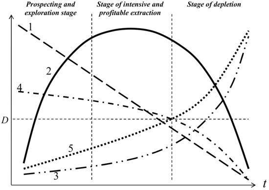
Figure 1.
Stages of mineral development and characteristic changes in indicators of the mineral resources and geological environment state 1—The ratio of inferred resources to minable reserves; 2—Total return on investment in exploration and operation; 3—The degree of involvement of secondary resources and substitutes; 4—Stability of the geological environment; 5—Costs for environmental protection and rehabilitation of territories; D—Assimilation potential of the geological environment.
The typical stages of deposit development are highlighted in Figure 1: 1—Prospecting and exploration stage; 2—Stage of intensive and profitable extraction; 3—Stage of depletion.
Stage 1 lasts from the start of exploration at the site and may include a trial production period or even lasts till reaching maximum production. Stage 1 is characterized by: (1) the presence of a large resource base, which is gradually being explored; this is expressed in the largest ratio of inferred resources to minable reserves; (2) a gradual increase in the return on investment in exploration while increasing reserves for future production; (3) little use of substitutes for raw materials, although their search and availability may take place; (4) the minimum values of the parameters of the environment change and costs for environmental protection and rehabilitation of territories. Stage 2 usually lasts from the moment of reaching maximum production until the moment of irreversible decline in production. During this period, resources turn into recoverable reserves, and their ratio gradually approaches one. After that, most of the investment in the exploration of reserves does not give the same return as in period 1. The scale of production is the cause of environmental changes and a significant increase in the cost of their stabilization. The third period begins from the moment of irreversible decline in production. This is characterized by the impossibility of increasing reserves due to their past extraction, deterioration in quality and concentration. This leads to an increase in operating costs when it becomes more profitable to use substitutes and conserve deposits.
This scheme is a theoretical distribution of the stages of resource development, but it gives a good idea of the need to model risks and the availability of raw materials in the implementation of new technological scenarios, especially when these scenarios are resource dependent.
Thus, the criticality of minerals is demonstrated with specific countries and specific minerals.
Measuring natural resource scarcity is the subject of considerable debate over which alternative indicators of scarcity, such as unit costs, prices, rents, the elasticity of substitution and energy costs, are better [20,23,24,31,32,33,34,35,36,37,38,39].
The main sources of data for determining the indices were: USGS statistics [40,41] on the amount of reserves and resources of metals as of 2019 and their consumption. We also used the data of the World Bank report [6], which related to the use of metals in green energy technologies and the forecast of their consumption in 2050.In the report, the classification of minerals was carried out, and the following groups were identified [6]:
- The first group of metals is not widely used in all renewable energy technologies but are key components of specific technologies, such as neodymium for wind energy and titanium for geothermal energy.
- The second group are minerals, the demand for which will increase several times and be accompanied by high risks in supply. These are graphite, cobalt and lithium, the reserves and production of which are monopolistically concentrated in some regions, and the consumption in others. Any potential problems in meeting this demand will cause changes in battery manufacturing and can affect battery chemistry or even battery type.
- The third group of metals, such as aluminium and iron, are critical due to their very widespread use; their demand does not depend on one particular technology, they are needed in huge quantities in a wide range of energy technologies. These metals are less prone to volatility and risk as high levels of demand for them will exist, regardless of what type of energy technology is deployed before 2050.
- The fourth group of metals (nickel, copper, chromium, manganese, etc.), the production of which, even without a significant increase in mineral demand, will be strongly affected by the transition to green energy. The supply of these metals will be risky due to their widespread use in other traditional industries.
Some studies deal with variation analysis of the combination of electricity and green gas, which offers several advantages in terms of efficiency and resources [42]. An example of a comprehensive assessment for various scenarios of the future development of a decentralized system of renewable energy sources is given in [43], which identified the main environmental disadvantages: an increase in the use of mineral resources and emissions of pollutants due to the necessary technical infrastructure and a significant increase in the use of resources for burning biomass.
Many recent studies also deal with the optimization of modern energy production facilities [44,45,46], but one of the key factors that are overlooked by the authors is the availability of critical raw materials and metals for these processes.
3. Method and Results
We propose the definition and scoring of availability indices as the product of 7 indices, which were determined when ranking minerals according to the parameters shown in Table 1.

Table 1.
Basic scoring indices.
The ranking of metals according to these characteristics was carried out, and the index of the availability of each mineral was determined. We classified 17 minerals that are critical in the green energy transition with the 10 main technologies.
To assess the risks of commodity limitations, we used an approach similar to the probability of success estimation often used in petroleum geology [47]. We consider all of the factors listed as important parts of the demand–supply system. Some assumptions were made to develop the scenario described below:
- All of the parameters are continuous functions, and it is possible to apply the linear or non-linear transformation of these functions;
- Proposed indices have no functional dependences and could be a fully or partially independent variable;
- There are no metals that have insurmountable risks in production during the forecasted period (the next 30 years). Therefore, the availability probability of success could be estimated in the range of 0.5–1.0 and show the value inverted to the risk.
- All estimations are relative and could be used for a comparison of different metals but do not demonstrate any absolute level of metal usage success.
- We do not account for any links between the metals mined from complex-type deposits (such as Ni-Cu-Co and Pb-Zn-Ag) due to the large variety of their genetic types. Additionally, we do not consider any facilities for joint metal production, which is inherent especially for base metals.
- Some of the metal is estimated by more detailed commodity-type (Aluminium from Bauxite, Titanium from Ilmenite and Rutile) or more integral (Neodymium as part of the Rare Earth Elements (REE) group) available data.
This comprehensive index makes it possible to highlight the most accessible metals and minerals with very limited access.
The initial data for calculating the availability indices are shown in the following Table 2 and Table 3.
Table 2.
Initial data for calculating the availability indices IA1, IA2 and IA3.
Table 3.
Initial data for calculating the availability indices IA4, IA5, IA6 and IA7.
To estimate the proposed indexed we used the following two-stage approach:
Stage I. We defined and gathered the data of the most significant attributes related to a selected parameter. For example, for Reserves IA, there were commodity reserves per thousand tons, annual mine production in 2019 and forecast of production for 2050—Depletion allowance by estimation of USGS. Based on this data, we calculated the period of reserves availability (in years) and the same period with correction for demand growth for 2050. As shown in Figure 2, there are two clusters of metals available, where the majority of them show a linear trend of low changes in availability, but three of them (lithium, graphite and vanadium) have a dramatically shortened availability compared to today.
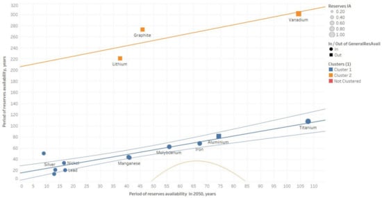
Figure 2.
Scatterplot of periods of metal reserves availability with and without correction fort he projected growth in demand in 2050. Colours show two identified clusters. Calculated Reserves IA (see explanation below) shown by symbol size. Linear trend lines and their confidence levels shown by bold and simple lines with colours corresponding to clusters.
This absolute value of years of availability was transformed to Reserves AI by linear transformation as with normalization in the range 0.5–1.0 explained above. Despite the lack of a statistically significant sample, we could recognize a lognormal behaviour of reserves and mine production attributes (see Figure 3), but their ratio represented by a period of reserves availability is linear and distributed relatively evenly.

Figure 3.
Bi-logarithmic scatterplot of metal reserves and mine production (projected with correction for demand growth in 2050). Circle size proportional to the period of reserves availability in years (with the correction for projected mine production in 2050). Colours show depletion allowance estimated by USGS.
To determine availability indices No.1–4 (Demand IA, Relative Demand IA, Technology IA, Emission IA) and No. 7 (Dominant Country, IA, USA), we used the linear transformation Equation (1)
where x—Selected attribute to describe the parameter; notation k, min and max correspond to current metal, minimal and maximal values of the selected attribute, respectively.
It was assumed that the larger the calculated indicator, the greater the risks in the availability of the resource.
To determine availability indices №№5–6 (Reserves IA and Diverse Country IA), it was assumed that the lower the calculated indicator, the greater the risks in the availability of the resource. Here, we used the linear transformation Equation (2)
where the notations in the formula are the same as in (1).
3.1. Ranking of Minerals by Demand Indicators
The ranking of minerals by demand indicators was carried out for the level of projected demand in 2050 when the transition to green energy is implemented. The absolute values of demand are important since the more metals are used in other directions, the lower their availability for new energy technologies.
Three groups of minerals were defined with a different order of numbers: 1 projected annual demand from energy technologies more than 1000 thousand tons, 2 projected annual demand from energy technologies more than 100 thousand tons and 3 projected annual demand from energy technologies more than 1 thousand tons. The ranking results are shown in Appendix C, Table A1.
3.2. Projected Annual Demand 2050 from Energy Technologies as a Percentage of the Current Rate
Additionally, the ranking was carried out according to the ratio of the growth in demand for metal in comparison with the current period. The higher it is, the greater the risks of mineral deficit. Three groups of minerals were defined with a different order of numbers: 1 projected annual demand from energy technologies of more than 100% of the current rate, 2 projected annual demand from energy technologies of more than 10% of the current rate, 3 projected annual demand from energy technologies of up to 10% of the current rate. The relationship between the projected 2050 annual demand and relative demand is demonstrated in Figure 4.
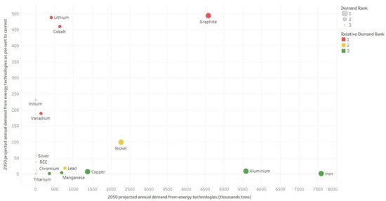
Notice that the distribution shown has no significant correlation. If the projection is correct, a shift in the structure of global metal production by the dramatic growth in graphite, lithium, cobalt, indium and vanadium production is expected. The ranking results are shown in Appendix C, Table A2.
3.3. Mineral Ranking with Relevant Low-Carbon Technologies
This ranking was carried out by the number of technologies where there is a need for an individual metal. The list of technologies includes the following: wind, solar photovoltaic, concentrated solar power, hydro, geothermal, energy storage, nuclear, coal, gas, carbon capture and storage. In total, we took into account 17 metals and minerals for 10 technologies (Figure 5).
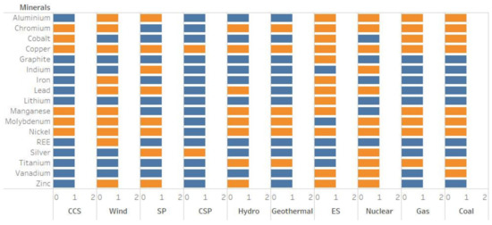
Figure 5.
Distribution of the relevant energy technologies. Column notations are the following: CCS—Carbon capture and storage; SP—Solar photovoltaic; CSP—Concentrated solar power; ES –energy storage. Commodity involved in technology marked by orange colour, not involved - blue one.
The ranking results are shown in Appendix C, Table A3.
3.4. Ranking of Minerals by Cumulative CO2 Emissions which Are Associated with Metal Production
To take into account the main environmental impact, we used total CO2 emissions in the production of metal. Figure 6 demonstrates a bi-logarithmic scatterplot of emissions versus reserves. The major contaminator is the production of iron/steel, then aluminium. The rest of the metals have no significant impact.
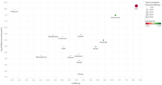
Figure 6.
Bi-logarithmic scatterplot of CO2 emissions versus reserves. Emission IA is shown by colour; symbol size corresponds to the total cumulative emission of carbon dioxide.
We used logarithmic transformation for cumulative carbon dioxide emissions. The ranking results are shown in Appendix C, Table A4.
3.5. Ranking of Minerals by the Period of Reserves Availability
For this ranking, we used indicators of reserves and productivity for minerals according to the data of the USGS [8,42]. The reserves were taken into account, since the resources require additional time for exploration and development. This period can take from 1–2 to 10 years. The calculation is based on reserves, as the most reliable resources prepared for mining. The original attributes, calculated parameters and ranking results are shown in Appendix C, Table A5.
Mine production with projected growth in 2050 was calculated as the product mine production in2019 and the corresponding value of increasing demand (column 3 Table A2).
where
- P2050—Mine production with projected growth in 2050;
- P2019—Mine production in 2019;
- R2050—Increasing demand rate up to 2050 % (column 3 Table A2).
The period of reserves availability was calculated by dividing minerals reserves and mine production with projected growth in 2050.
where
- P2050—Mine production with projected growth in 2050;
- Tonnage—Metals and minerals reserves in thousand t.
3.6. Ranking of Minerals by the Number of Countries That Produced More Than 1% of Global Production
Ranking was based on mineral commodity indices of countries’ productivity in 2019. The ranking results are shown in Appendix C, Table A6.
Additional systematization of the 7 availability indices was performed to take into account the monopolization of mineral extraction. The maximum production of each country was defined. Indium is the most commonly recovered from the zinc–sulphide ore mineral sphalerite; the value of its index was equated to zinc. The ranking results are shown in Appendix C, Table A7.
The spatial distribution of countries with a dominating position in different commodities markets is demonstrated in Figure 7.
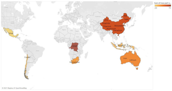
Figure 7.
The spatial distribution of commodities with a significant annual production concentrated in each country.
Stage 2. To calculate the integral score of the defined availability indices, we used two scenarios: full independent variables and partially dependent variables.
Scenario 1.
The first approach of our probabilistic estimation was accounting for all 7 of the defined indices as mandatory and fully independent parts of a successful demand–supply system. We did not have any significant criteria to estimate the weight of each IA; we thus estimated the integral score as the product of all available parameters:
where the notation is the same as in (1).
This approach has some disadvantages related to obvious linkages between some of the parameters. However, the regressive analysis shown in the scatterplot in Appendix D (Figure A9) did not demonstrate any significant correlation between the parameters. Additionally, we had a lack of data for reserves of indium and neodymium (Appendix C, Table A1), which forced us to exclude one index in formula (5) or replace values of Reserves AI with 1.0. Certainly, this shifted the final integral estimation described below.
The total availability index was calculated as the product of the 7 defined indices (Appendix C, Table A1, Table A2, Table A3, Table A4, Table A5, Table A6 and Table A7) and comprehensively took into account the risk of limited access to mineral reserves. The result is shown in Table 4, where green colour say about the full availability, red—About low one.
Table 4.
Total availability index by minerals.
Scenario 2.
In scenario 2, we realized the compromise approach between data-driven and expert-driven estimation. The impact of different indices could be grouped by risk types (supply risk, demand risk and geopolitics risk). Relationships between the groups were probabilistically weaker than within the groups. To estimate the integral probability of success of such demand–supply system, we used a fuzzy logic model developed by [48] and heavily expanded in modern mineral prospective modelling practice [49,50,51,52,53].
We developed the fuzzy logic model (Figure 8), which consist of three steps:
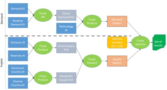
Figure 8.
Fuzzy logic model for Scenario 2.
- Grouping of availability indices and estimation of intermediate parameters named “direct demand probability of success (PoS)”, “direct supply PoS” and “Geopolitics supply PoS” by using Fuzzy operators;
- The second intermediate level combines the results of the previous level and estimates “Demand system” and “Supply system”;
- Final estimation of balance between the demand and supply systems by using the fuzzy gamma operator where gamma is the variable impacts on the weights of each system in the final result. There was a set of 9 models obtained with a gamma range from 0.1 to 0.9 with a step of 0.1.
Fuzzy operators used in the model were calculated using the following definitions:
Fuzzy OR operator is equal to the maximum from the set function:
where µi is the input data.
The fuzzy product operator is calculated by the following formula:
The fuzzy sum operator is calculated by the following formula:
Finally, the fuzzy gamma operator is calculated by the following formula:
The fuzzy AND operator is equal to the minimum from the set function but was not used here.
The input data in Scenario 2 were the same as in Scenario 1. The results of the fuzzy set calculation are demonstrated in Table 5, Table 6 and Table 7.
Table 5.
Result of calculation of intermediate levels of demand system in Scenario 2 fuzzy model.
Table 6.
Result of calculation of intermediate levels of supply system in Scenario 2 fuzzy model.
Table 7.
Result of calculation of the final level of in Scenario 2 fuzzy model. For a focused view, the results of gamma 0.2, 0.4, 0.6 and 0.8 were removed.
The different estimations in Table 7 are linearly dependent on the gamma variable. We calculated the deviation as a result of the model gamma = 0.1 (supply risky case) subtracted gamma = 0.9 model (demand risky case) as an attribute of metal “volatility” in the demand–supply system. Additionally, we compared these results with the result of Scenario 1 (Table 8).
Table 8.
Comparison of results of Scenario 1 and Scenario 2.
4. Discussion
These classifications can be detailed regionally and locally for each country. For the example of Ukraine, the indices of the availability of reserves for titanium and iron will be much better than the global ones. When using such country-specific instruments, the list of indicators should be complemented by those that are imported in large quantities. Here, the primary risk will be undiversified supplies from one source, from one country. Certainly, the approach in this paper could be expanded in the direction of the better reflection of profitable methods of carbon sequestration. Along with this milestone, more econometric methods could be incorporated into forecasting analyses, but this paper sheds light on the incorporation of mathematically sophisticated methods into the urgent question of the mineral policy.
Indicators of social and economic importance, as well as regulatory restrictions for the extraction and processing of raw materials, are especially relevant. The social effects that arise from traditional mining business practices can be heavily offset by aspects of mineral scarcity. The lack of quantity and quality of minerals and geopolitical supply risks lead to higher prices, which in turn makes it possible to use smart mining technologies. The presence of smart technologies and the awareness of the mineral scarcity for strategic industries made it possible to resume geological exploration and mining, even in regions where they were mothballed.
However, the most important factor is not just the technological impact but the social one. According to the European Commission’s definition given to social innovation, we extensively frame it as an advantageous or win–win interdependence process among four pillars: social actors, technology, environment and economy, where “new ideas meet social needs, create social relationships and form new collaborations” [54,55,56].
In this respect, key policy recommendations within the framework of limited critical resources and a green energy transition could include:
- Understanding differences in technologies concerning size; component configuration; chemistry; material composition; and other factors that might impact the energy, environmental and cost impacts of recycling these materials;
- Analysing and supporting current, near-term (5–10 years) and future commercial processes being used or that could be used for the recycling and reuse of these material-based products at their end-of-useful life;
- Identifying the potential technical, environmental, cost and energy impacts associated with the recycling of these materials and second-life applications, including any engineering or financial obstacles or other barriers;
- Acknowledging and tackling gaps and areas that could be further investigated;
- Documenting and prioritizing the study findings in a laid out and easy-to-follow report clearly fulfilling the key “refurbish, reuse, recycle”, circular economy principle.
Some new mineral recycling technologies that are currently in development attempt to increase the recovery rate for various metals, such as cobalt and nickel, through the recycling system. These technologies focus on hydrometallurgical processes, which are less energy intensive than pyrometallurgical processes. The new recycling technologies commit to increasing recycling rates to a reported 90%+. The companies developing these new recycling technologies are most interested in direct recycling or cathode-to-cathode recycling to recover chemicals and chemical powders suitable for direct sale back to initial product manufacturers. However, none of these technologies is yet operating at scale, which is the current challenge [57].
To assess the progress of a transition process, one must measure the status quo and compare it with previous phases. Using a numeric value for a global indicator can ease the reporting process and enhance the overview of decisionmakers [55]. Other researchers [56] have proposed flexible and adaptable software tools to simplify the sustainability reporting process, allowing the user to easily calculate established or custom indices by effortlessly computing various indicators, which can be applied to assess how the key policy recommendations have been applied. Economies are shifting towards a system where the main efforts are should regenerate natural systems, design waste, pollution decrease and keep products and materials in use. This process would make the shift from the old linear economy to towards the circular one [58]. Thus, based on the present research, a practical question arises: what is the relevance of the circular economy to businesses, thus considering mineral usage under limited critical resources and a green energy transition? The major modern for-profit business orientation requires a new approach where the balance between the environmental benefits of recycling [59,60], such as the better use of resources and lower carbon emissions, and reuse—Known as “second life” applications, should converge [61,62,63].
Proper regulation and policy tools would lead to direct recycling, consequently quickly becoming the coherent route of the circular economy. The human-made world should turn towards making use of renewable energy instead of hydrocarbons. This principle should be based on numerous actors working together to create effective flows of materials and information.
5. Conclusions
Two scenarios presented in the current research expose a high level of uncertainty of the projected 2050 forecast. Furthermore, despite different methodologies, it is possible to rank the selected 17 commodities by the integral probability of success. Such estimation is relative but could push a commodity exploration strategy both for governments and commercial companies.
Scenario 1 is more conservative and realizes the data-driven static model with the lowest level of PoS. The lowest availability index values (up to 0.15) were calculated for cobalt, graphite and lithium, which are key battery minerals. This is a consequence of a significant increase in demand for green energy and a high mining concentration in one region. Low indices (up to 0.20) were also obtained for iron, nickel and chromium. For nickel and chromium, the explored and prepared for mining reserves limitations are most influential. Reserves availability periods of the metals were calculated with the current and forecasted demand. These periods for Ni and Cr are13 and 17 years, respectively, which are less than the optimal life of one large mine. Considering that the development of a new mining facility at its design capacity lasts from 4 to 7 years, a group of minerals (cobalt, chromium, silver zinc, lead and nickel) with a period of less than 20 years is the riskiest. The criticality of metals such as iron, copper and aluminium is associated with their huge volumes of use in other traditional industries, but for iron, the most acute factor is the depletion of high-grade ores.
Titanium and indium have the highest availability indices. The first is due to a slight increase in demand and resource abundance, as well as easy mining and processing. The results for indium can be considered insufficiently accurate. Indium is most commonly recovered from the zinc–sulphide ore mineral sphalerite, but the source materials lacked systematic data on indium reserves and mine production.
The availability index provides an opportunity to determine the degree of risk associated not only with the availability of resources but also with the risks of disruptions in the supply chain. These indicators do not assess the rarity of metals in nature but assess the risks of the availability of their required quantity and quality in the implementation of green energy.
The list of indices that are used in the calculation makes it possible to overcome the most vulnerable issues in the short- and long-term consumption of metals in green energy technologies.
The metals that will be used in the largest quantities were highlighted—Iron, aluminium, graphite, nickel and copper—Among which the growth in consumption of certain metals in the energy sector will increase by more than 50% (graphite, nickel, cobalt, etc.). For nickel and cobalt, this is also accompanied by a limited reserve period of up to 20 years. This is and will be the motivation for investing in geological exploration or searching for substitutes.
Scenario 2 presents a more flexible combination of data-driven and expert-driven approaches. The main idea of fuzzy estimation is to show a range of potential changes in the balance between demand and supply. There are many factors that could dramatically change the global balance: not only the current global COVID-19 pandemic but the energy demand growth due to hidden crypto-currency mining (including high demand for excellent electronics chips), political wavering in the question of Earth climate changes, other energy types at the regional level, etc. Separately, we need to mention “third power” in nuclear energy. This is only one field where significant scientific progress, such as small nuclear (uranium or thorium) reactors, is possible and realistic in the projected period. This could spread the whole development worldwide.
The set of fuzzy models in general shows that the supply system is more critical for commodities. The model with gamma = 0.1 shows a similar estimation to that in Scenario 1, but is slightly more optimistic for iron, aluminium, lithium, graphite and indium. The demand risk-dominated model with gamma = 0.9 shows the most positive estimation of success (all scores are greater than 0.6). However, we noticed here that chromium and nickel have the lowest scores due to being involved in a large number of technologies in combination with the relatively risky supply. Copper, molybdenum and manganese compensate for high demand risks by sufficient supply.
The changes in the demand–supply balance for any reason described above or elsewhere will impact commodities differently. The most volatile group with regard to our estimation consists of cobalt, lithium, REE plus ferrous metals iron and vanadium.
Author Contributions
Conceptualization, M.K., O.L. and G.K.; methodology, M.K. and O.L.; software, G.K., P.N. and O.L.; validation, S.N., M.K., O.L. and G.K.; formal analysis, O.L.; investigation, O.L. and M.K.; resources, G.K. and S.N.; data curation, O.L., P.N. and G.K.; writing—Original draft preparation, M.K. and O.L.; writing—Review and editing, G.K., Y.B., P.N. and S.N.; visualization, M.K. and O.L.; supervision, S.N.; project administration, G.K., Y.B. and S.N.; funding acquisition, S.N. and Y.B. All authors have read and agreed to the published version of the manuscript.
Funding
Project financed by Lucian Blaga University of Sibiu research grants LBUS-IRG-2019-05. This research was carried out as a part of project no. POIR.01.01.01-00-0281/20-00, entitled: “Predictive energy management system En MS”, co-financed by the National Center for Research and Development.
Institutional Review Board Statement
Not applicable.
Informed Consent Statement
Not applicable.
Data Availability Statement
Free open sources of data were used.
Acknowledgments
Data warehouse development, data transformation and visualization were performed with the IBM Tableau academic license in Taras Shevchenko National University of Kyiv, Ukraine.
Conflicts of Interest
The authors declare no conflict of interest.
Appendix A. Global Mine Production of Some Critical Minerals and Metals

Figure A1.
Global mine production of Co per thousand tons (build on the data from [25]), the red line is a trend.
Figure A1.
Global mine production of Co per thousand tons (build on the data from [25]), the red line is a trend.


Figure A2.
Global mine production of Li per thousand tons (build on the data from [25]), the red line is a trend.
Figure A2.
Global mine production of Li per thousand tons (build on the data from [25]), the red line is a trend.


Figure A3.
Global mine production of graphite per thousand tons (build on the data from [25]), the red line is a trend.
Figure A3.
Global mine production of graphite per thousand tons (build on the data from [25]), the red line is a trend.


Figure A4.
Global mine production of copper per thousand tons (build on the data from [25]), the red line is a trend.
Figure A4.
Global mine production of copper per thousand tons (build on the data from [25]), the red line is a trend.

Appendix B

Figure A5.
Co price dynamics in USD/t (build on the data from [25]), the red line is a trend.
Figure A5.
Co price dynamics in USD/t (build on the data from [25]), the red line is a trend.


Figure A6.
Li price dynamics, battery-grade lithium carbonate, in USD/t (build on the data from [25]).
Figure A6.
Li price dynamics, battery-grade lithium carbonate, in USD/t (build on the data from [25]).


Figure A7.
Graphite price dynamics in USD/t (build on the data from [25]).
Figure A7.
Graphite price dynamics in USD/t (build on the data from [25]).


Figure A8.
Copper price dynamics in USD/t (build on the data from [25]), the red line is a trend.
Figure A8.
Copper price dynamics in USD/t (build on the data from [25]), the red line is a trend.

Appendix C
Table A1.
Mineral ranking by 2050 projected annual demand indicators.
Table A1.
Mineral ranking by 2050 projected annual demand indicators.
| Ranking | Minerals | 2050 Projected Annual Demand from Energy Technologies, Thousand Tons (According to Data [6]) | IA1 |
|---|---|---|---|
| 1 projected annual demand from energy technologies more than 1000 thousand tons | Iron | 7584 | 0.50 |
| Aluminium | 5583 | 0.63 | |
| Graphite | 4590 | 0.70 | |
| Nickel | 2268 | 0.85 | |
| Copper | 1378 | 0.91 | |
| 2 projected annual demand from energy technologies more than 100 thousand tons | Lead | 781 | 0.95 |
| Manganese | 694 | 0.95 | |
| Cobalt | 644 | 0.96 | |
| Lithium | 415 | 0.97 | |
| Chromium | 366 | 0.98 | |
| Vanadium | 138 | 0.99 | |
| 3 projected annual demand from energy technologies more than 1 thousand tons | Molybdenum | 33 | 1.00 |
| Silver | 15 | 1.00 | |
| Neodymium | 8.4 | 1.00 | |
| Titanium | 3.44 | 1.00 | |
| Indium | 1.73 | 1.00 |
Table A2.
Ranking of minerals by demand indicators аs a percentage of the current rate.
Table A2.
Ranking of minerals by demand indicators аs a percentage of the current rate.
| Ranking | Minerals | 2050 Projected Annual Demand from Energy Technologies as a Percentage of the Current Rate (According to Data [6]) | IA2 |
|---|---|---|---|
| 1 projected annual demand from energy technologies more than 100% of the current rate | Graphite | 494 | 0.50 |
| Lithium | 488 | 0.51 | |
| Cobalt | 460 | 0.53 | |
| Indium | 231 | 0.77 | |
| Vanadium | 189 | 0.81 | |
| 2 projected annual demand from energy technologies more than 10% of the current rate | Nickel | 99 | 0.90 |
| Silver | 56 | 0.94 | |
| Neodymium | 37 | 0.96 | |
| Lead | 18 | 0.98 | |
| Molybdenum | 11 | 0.99 | |
| 3 projected annual demand from energy technologies up to 10% of the current rate | Aluminium | 9 | 0.99 |
| Copper | 7 | 0.99 | |
| Manganese | 4 | 1.00 | |
| Chromium | 1 | 1.00 | |
| Iron | 1 | 1.00 | |
| Titanium | 0 | 1.00 |
Table A3.
Ranking of minerals by demand indicators from relevant low-carbon technologies.
Table A3.
Ranking of minerals by demand indicators from relevant low-carbon technologies.
| Minerals | Number of Technologies (According to Data [6]) | Relevant Low-Carbon Technologies | IA3 |
|---|---|---|---|
| Copper | 10 | wind, solar photovoltaic, concentrated solar power, hydro, geothermal, energy storage, nuclear, coal, gas, carbon capture and storage | 0.50 |
| Nickel | 9 | wind, solar photovoltaic, hydro, geothermal, energy storage, nuclear, coal, gas, carbon capture and storage | 0.56 |
| Molybdenum | 8 | wind, solar photovoltaic, hydro, geothermal, nuclear, coal, gas, carbon capture and storage | 0.61 |
| Chromium | 8 | wind, hydro, geothermal, energy storage, nuclear, coal, gas, carbon capture and storage | 0.61 |
| Manganese | 7 | wind, hydro, geothermal, energy storage, coal, gas, carbon capture and storage | 0.67 |
| Aluminium | 6 | wind, solar photovoltaic, energy storage, nuclear, coal, gas | 0.72 |
| Titanium | 6 | hydro, geothermal, nuclear, coal, gas | 0.72 |
| Lead | 5 | wind, solar photovoltaic, hydro, energy storage, nuclear | 0.78 |
| Zinc | 5 | wind, solar photovoltaic, hydro, energy storage, nuclear | 0.78 |
| Cobalt | 4 | energy storage, coal, gas, carbon capture and storage | 0.83 |
| Silver | 3 | solar photovoltaic, concentrated solar power, nuclear | 0.89 |
| Vanadium | 3 | energy storage, nuclear, coal | 0.89 |
| Indium | 2 | solar photovoltaic, nuclear | 0.94 |
| Iron | 2 | wind, energy storage | 0.94 |
| Graphite | 1 | energy storage | 1.00 |
| Lithium | 1 | energy storage | 1.00 |
| Neodymium | 1 | wind | 1.00 |
Table A4.
Mineral ranking by cumulative CO2 emissions which are associated with metal production.
Table A4.
Mineral ranking by cumulative CO2 emissions which are associated with metal production.
| Minerals | Total Cumulative Emissions MtCO2E (According to Data [6]) | Ln MtCO2E | IA4 |
|---|---|---|---|
| Iron/steel | 3655.4 | 8.20 | 0.50 |
| Aluminium | 842.7 | 6.74 | 0.89 |
| Graphite | 363.5 | 5.90 | 0.95 |
| Nickel | 211.6 | 5.35 | 0.97 |
| Zinc | 93.7 | 4.54 | 0.99 |
| Copper | 73.7 | 4.30 | 0.99 |
| Cobalt | 66.5 | 4.20 | 0.99 |
| Vanadium | 63 | 4.14 | 0.99 |
| Silver | 60.7 | 4.11 | 0.99 |
| Lithium | 36.4 | 3.59 | 1.00 |
| Lead | 22.3 | 3.10 | 1.00 |
| Chromium | 20.4 | 3.02 | 1.00 |
| Manganese | 10.6 | 2.36 | 1.00 |
| Molybdenum | 4.7 | 1.55 | 1.00 |
| Indium | 3.4 | 1.22 | 1.00 |
| Neodymium | 2.9 | 1.06 | 1.00 |
| Titanium | 0.7 | −0.36 | 1.00 |
Table A5.
Mineral ranking by the period of reserves availability.
Table A5.
Mineral ranking by the period of reserves availability.
| Minerals | Reserves According to Data [40], Thousand Tons | Mine Production 2019 According to Data [40], Thousand Tons Per Year | Mine Production with Projected Growth in 2050, Thousand Tons Per Year | Period of Reserves Availability with Projected Growth in 2050, Years (as Column 2/Column 4) | IA5 |
|---|---|---|---|---|---|
| 1 | 2 | 3 | 4 | 5 | 6 |
| Titanium | 82,000,000 | 760,000 | 760,000 | 108 | 1.00 |
| Vanadium | 22,000 | 73 | 211 | 104 | 0.98 |
| Aluminium/Bauxite Mine Production | 30,000,000 | 370,000 | 403,300 | 74 | 0.83 |
| Iron | 170,000,000 | 2,500,000 | 2,525,000 | 67 | 0.80 |
| Molybdenum | 18,000 | 290 | 322 | 56 | 0.74 |
| Graphite | 300,000 | 1100 | 6534 | 46 | 0.69 |
| Manganese | 810,000 | 19,000 | 19,760 | 41 | 0.66 |
| Copper | 870,000 | 20,000 | 21,400 | 41 | 0.66 |
| Lithium | 17,000 | 77 | 453 | 38 | 0.64 |
| Zinc | 250,000 | 13,000 | 13,003 | 19 | 0.55 |
| Lead | 90,000 | 4500 | 5310 | 17 | 0.54 |
| Nickel | 89,000 | 2700 | 5373 | 17 | 0.54 |
| Silver | 560 | 27 | 42 | 13 | 0.52 |
| Chromium | 570,000 | 44,000 | 44,440 | 13 | 0.52 |
| Cobalt | 7000 | 140 | 784 | 9 | 0.50 |
| Neodymium | n/a | n/a | |||
| Indium | n/a | n/a |
Table A6.
Ranking of minerals by the number of countries that produced more than 1% of global production.
Table A6.
Ranking of minerals by the number of countries that produced more than 1% of global production.
| Minerals | Number of Countries that Produced More Than 1% | IA6 |
|---|---|---|
| Iron | 10 | 1.00 |
| Aluminium/Bauxite Mine Production | 10 | 1.00 |
| Graphite | 10 | 1.00 |
| Copper | 10 | 1.00 |
| Lead | 10 | 1.00 |
| Zinc | 10 | 1.00 |
| Manganese | 10 | 1.00 |
| Cobalt | 10 | 1.00 |
| Silver | 10 | 1.00 |
| Titanium | 10 | 1.00 |
| Nickel | 9 | 0.92 |
| Molybdenum | 9 | 0.92 |
| Indium | 8 | 0.83 |
| Lithium | 6 | 0.67 |
| Chromium | 6 | 0.67 |
| REE total, incl. Neodymium | 6 | 0.67 |
| Vanadium | 4 | 0.50 |
Table A7.
Ranking of minerals for each country with max annual productivity.
Table A7.
Ranking of minerals for each country with max annual productivity.
| Minerals | Max Annual Productivity | Countries with Max Annual Productivity | IA7 |
|---|---|---|---|
| Cobalt | 70 | Democratic Republic of Congo | 0.50 |
| REE total, incl. Neodymium | 67 | China | 0.53 |
| Graphite | 64 | China | 0.56 |
| Aluminium /Bauxite Mine Production | 57 | China | 0.64 |
| Lithium | 55 | Australia | 0.66 |
| Vanadium | 55 | China | 0.66 |
| Lead | 47 | China | 0.74 |
| Molybdenum | 45 | China | 0.77 |
| Iron | 39 | Australia | 0.83 |
| Chromium | 38 | South Africa | 0.84 |
| Zinc | 33 | China | 0.89 |
| Indium | 33 | 0.89 | |
| Nickel | 30 | Indonesia | 0.93 |
| Manganese | 29 | South Africa | 0.94 |
| Copper | 28 | Chile | 0.95 |
| Titanium incl. | 27 | China | 0.96 |
| Silver | 23 | Mexico | 1.00 |
Appendix D

Figure A9.
Cross-correlation scatterplot of availability indices. Grey lines correspond to linear trend and confidence bands.
Figure A9.
Cross-correlation scatterplot of availability indices. Grey lines correspond to linear trend and confidence bands.

References
- Hernandez-Serrano, P.V.; Zaveri, A. Venturing the Definition of Green Energy Transition: A systematic literature review. arXiv 2020, arXiv:2004.10562. [Google Scholar]
- Mills, M.P. The New Energy Economy: An Exercise in Magical Thinking; Manhattan Institute for Policy Research: New York, NY, USA, 2019. [Google Scholar]
- Kumar, S.V. National Mineral Policy 2019: A Remedy as Bad as the Disease? Ecol. Econ. Soc. INSEE J. 2020, 3, 111–114. [Google Scholar]
- Basu, R. Conversations on National Mineral Policy 2019: Will intergenerational equity be implemented? Ecol. Econ. Soc. INSEE J. 2020, 3, 115–118. [Google Scholar]
- Bogdanov, D.; Ram, M.; Aghahosseini, A.; Gulagi, A.; Oyewo, A.S.; Child, M.; Caldera, U.; Sadovskaia, K.; Farfan, J.; Barbosa, L.D.; et al. Low-cost renewable electricity as the key driver of the global energy transition towards sustainability. Energy 2021, 227, 120467. [Google Scholar] [CrossRef]
- Hund, K.; la Porta, D.; Fabregas, T.P.; Laing, T.; Drexhage, J. Minerals for Climate Action: The Mineral Intensity of the Clean Energy Transition; International Bank for Reconstruction and Development, The World Bank, 2020. Available online: http://www.eqmagpro.com/wp-content/uploads/2020/05/MineralsforClimateActionTheMineralIntensityoftheCleanEnergyTransition_compressed-1-18.pdf (accessed on 14 December 2020).
- Razmjoo, A.; Gakenia-Kaigutha, L.; Vaziri-Rad, M.A.; Marzband, M.; Davarpanah, A.; Denai, M. A Technical analysis investigating energy sustainability utilizing reliable renewable energy sources to reduce CO2 emissions in a high potential area. Renew. Energy 2021, 164, 46–57. [Google Scholar] [CrossRef]
- Zhang, B.; Peng, S.; Xu, X.; Wang, L. Embodiment Analysis for Greenhouse Gas Emissions by Chinese Economy Based on Global Thermodynamic Potentials. Energies 2011, 4, 1897–1915. [Google Scholar] [CrossRef]
- Smol, M.; Marcinek, P.; Duda, J.; Szołdrowska, D. Importance of sustainable mineral resource Management in Implementing the circular economy (CE) model and the European green Deal strategy. Resources 2020, 9, 55. [Google Scholar] [CrossRef]
- Ghosh, S.K. Circular Economy: Global Perspective; Springer: Berlin/Heidelberg, Germany, 2020. [Google Scholar]
- Smol, M.; Adam, C.; Preisner, M. Circular economy model framework in the European water and wastewater sector. J. Mater. Cycles Waste Manag. 2020, 22, 682–697. [Google Scholar] [CrossRef]
- Peiry, L.T.; Mundez, G.V. Material and Energy Requirement for Rare Earth Production. J. Miner. Met. Mater. Soc. JOM 2013, 65, 1327–1340. [Google Scholar] [CrossRef]
- Gutowski, T.G.; Sahni, S.; Allwood, J.M.; Ashby, M.F.; Worrell, E. The Energy Required to Produce Materials: Constraints on Energy-Intensity Improvements, Parameters of Demand. Philos. Trans. R. Soc. A Math. Phys. Eng. Sci. 2013, 371, 20120003. [Google Scholar] [CrossRef] [PubMed]
- Nate, S.; Bilan, Y.; Cherevatskyi, D.; Kharlamova, G.; Lyakh, O.; Wosiak, A. The Impact of Energy Consumption on the Three Pillars of Sustainable Development. Energies 2021, 14, 1372. [Google Scholar] [CrossRef]
- Stavytskyy, A.; Kharlamova, G.; Giedraitis, V.; Šumskis, V. Estimating the interrelation between energy security and macroeconomic factors in European countries. J. Int. Stud. 2018, 11, 217–238. [Google Scholar] [CrossRef] [PubMed]
- Beylot, A.; Guyonnet, D.; Muller, S.; Vaxelaire, S.; Villeneuve, J. Mineral raw material requirements and associated climate-change impacts of the French energy transition by 2050. J. Clean. Prod. 2019, 208, 1198–1205. [Google Scholar] [CrossRef]
- Goyal, S.; Esposito, M.; Kapoor, A. Circular economy business models in developing economies: Lessons from India on reduce, recycle, and reuse paradigms. Thunderbird Int. Bus. Rev. 2018, 60, 729–740. [Google Scholar] [CrossRef]
- Ciriminna, R.; Albanese, L.; Meneguzzo, F.; Pagliaro, M. Hydrogen peroxide: A key chemical for today’s sustainable development. ChemSusChem 2016, 9, 3374–3381. [Google Scholar] [CrossRef]
- Hotelling, H. The Economics of Exhaustible Resources. J. Political Econ. 1931, 39, 137–175. [Google Scholar] [CrossRef]
- Bretschger, L. Economics of technological change and the natural environment: How effective are innovations as a remedy for resource scarcity? Ecol. Econ. 2005, 54, 148–163. [Google Scholar] [CrossRef]
- Brown-Stephen, P.A.; Wolk, D. Natural resource scarcity and technological change. Econ. Financ. Policy Rev. 2000, 2–13. Available online: http://www.dallasfed.org/assets/documents/research/efr/2000/efr0001a.pdf (accessed on 10 December 2020).
- Wright, G.; Czelusta, J. Resources Based Economic Growth, Past and Present; Stanford University: Stanford, CA, USA, 2002; Available online: https://econweb.ucsd.edu (accessed on 7 December 2020).
- Kraut-Kraemer, J.A. Economics of Natural Resource Scarcity: The State of the Debate. Discussion Papers 10562, Resources for the Future. 2005. Available online: https://media.rff.org/documents/RFF-DP-05-14.pdf (accessed on 4 December 2020).
- Van Veldhuizen, R.; Sonnemans, J. Non-Renewable Resources, Strategic Behavior and the Hotelling Rule: An Experiment, Discussion Papers, Research Unit: Market Behavior. SP II 2014-203, WZB Berlin Social Science Center. 2014. Available online: https://www.econstor.eu/bitstream/10419/96220/1/782849776.pdf (accessed on 3 December 2020).
- Assessment of Critical Minerals: Updated Application of Screening Methodology. A Report by the Subcommittee on Critical and Strategic Mineral Supply Chains Committee on Environment, Natural Resources, and Sustainability. The National Science and Technology Council. 2018. Available online: https://www.whitehouse.gov/wp-content/uploads/2018/02/Assessment-of-Critical-Minerals-Update-2018.pdf (accessed on 30 November 2020).
- Critical Raw Materials Resilience: Charting a Path Towards Greater Security and Sustainability. Communication from the Commission to the European Parliament, the Council, the European Economic and Social Committee and the Committee of the Regions. COM (2020) 474 Final. Brussels, 3.9. 2020. Available online: https://eur-lex.europa.eu/legal-content/EN/TXT/PDF/?uri=CELEX:52020DC0474&from=EN (accessed on 30 November 2020).
- Fortier, S.M.; Nassar, N.T.; Lederer, G.W.; Brainard, J.; Gambogi, J.; McCullough, E.A. Draft Critical Mineral List—Summary of Methodology and Background Information—U.S. Geological Survey Technical Input Document in Response to SECRETARIAL Order No. 3359; U.S. Geological Survey Open-File Report 2018-1021; U.S. Geological Survey Open: Reston, VA, USA, 2018; 15p. [Google Scholar] [CrossRef]
- Neumayer, E. Scarce or abundant? The economics of natural resource availability. J. Econ. Surv. 2000, 14, 307–335. [Google Scholar] [CrossRef]
- Hanley, N.; Shogren, J.F.; White, B. Natural Resources: Types, Classification and Scarcity. In Environmental Economics in Theory and Practice; Macmillan Texts in Economics; Springer, Palgrave: London, UK, 1997; pp. 216–226. [Google Scholar] [CrossRef]
- Dovgy, S.O.; Shestopalov, V.M.; Korzhnev, M.M.; Trofimchuk, O.M.; Yakovlev, E.A. Restructuring of the Mineral Resource Base of Ukraine and Its Information Support; Institute of Telecommunications and Global Information Space, Scientific Opinion: Kyiv, Ukraine, 2007; pp. 78–84. [Google Scholar]
- Cleveland, C.J.; Stern, D.I. Indicators of natural resource scarcity: Review, synthesis, and application to US agriculture. In Theory and Implementation of Economic Models for Sustainable Development; van den Bergh, J.C.J.M., Hofkes, M.W., Eds.; Springer: Dordrecht, The Netherlands, 1998; Volume 15. [Google Scholar] [CrossRef]
- Farzin Hossein, Y. The Effect of the Discount Rate on Depletion of Exhaustible Resources. J. Political Econ. 1984, 92, 841–851. [Google Scholar] [CrossRef]
- Jägemann, C.C. Essays on the Economics of Decarbonization and Renewable Energy Support. Doctoral Dissertation, University of Cologne, Cologne, Germany, 2014. Available online: https://inis.iaea.org/collection/NCLCollectionStore/_Public/47/042/47042515.pdf (accessed on 30 November 2020).
- Mirman, L.J.; Spulber, D.F. Essays in the Economics of Renewable Resources; Elsevier Science Pub. Co.: Amsterdam, The Netherlands, 1982. [Google Scholar]
- Pindyck-Robert, S. Interfuel Substitution and the Industrial Demand for Energy: An International Comparison. Rev. Econ. Stat. 1977, 61, 169–179. [Google Scholar] [CrossRef]
- Pindyck-Robert, S. The Optimal Exploration and Production of Nonrenewable Resources. J. Political Econ. 1978, 86, 841–861. [Google Scholar]
- Chari, V.V.; Lawrence, J.C. The Optimal Extraction of Exhaustible Resources. Economic Policy Paper 14-5. Federal Reserve Bank of Minneapolis. 2014. Available online: https://www.minneapolisfed.org/~/media/files/pubs/eppapers/14-5/eppaper14-5.pdf (accessed on 30 November 2020).
- Withagen, C. The optimal exploitation of exhaustible resources, a survey. De Econ. 1981, 129, 504–531. [Google Scholar] [CrossRef]
- Young, D. Cost Specification and Firm Behaviour in a Hotelling Model of Resource Extraction. Can. J. Econ. Rev. Can. D’Economique 1992, 25, 41–59. [Google Scholar] [CrossRef]
- Commodity Statistics and Information, Mineral Commodity Summaries. In National Minerals Information Center; U.S. Geological Survey: Reston, VA, USA, 2020. [CrossRef]
- U.S. Geological Survey. Mineral Commodity Summaries 2020; U.S. Department of the Interior: Washington, DC, USA, 2020. [CrossRef]
- De Maered’Aertrycke, G.; Smeers, Y.; de Peufeilhoux, H.; Lucille, P.-L. The Role of Electrification in the Decarbonization of Central-Western Europe. Energies 2020, 13, 4919. [Google Scholar] [CrossRef]
- Lambrecht, H.; Lewerenz, S.; Hottenroth, H.; Tietze, I.; Viere, T. Ecological Scarcity Based Impact Assessment for a Decentralised Renewable Energy System. Energies 2020, 13, 5655. [Google Scholar] [CrossRef]
- Li, M.; Xu, Y.; Guo, J.; Li, Y.; Li, W. Application of a GIS-Based Fuzzy Multi-Criteria Evaluation Approach for Wind Farm Site Selection in China. Energies 2020, 13, 2426. [Google Scholar] [CrossRef]
- Petrenko, Y.; Denisov, I.; Koshebayeva, G.; Biryukov, V. Energy Efficiency of Kazakhstan Enterprises: Unexpected Findings. Energies 2020, 13, 1055. [Google Scholar] [CrossRef]
- Rabe, M.; Streimikiene, D.; Bilan, Y. Model of Optimization of Wind Energy Production in the Light of Legal Changes in Poland. Energies 2020, 13, 1557. [Google Scholar] [CrossRef]
- Davis, J.C. Estimation of the probability of success in petroleum exploration. Math. Geol. 1977, 9, 409–427. [Google Scholar] [CrossRef]
- Zadeh, L.A. Fuzzysets. Inf. Control 1965, 8, 338–353. [Google Scholar] [CrossRef]
- An, P.; Moon, W.M.; Rencz, A. Application of fuzzy set theory for integration of geological, geophysical and remote sensing data. Can. J. Explor. Geophys. 1991, 27, 1–11. [Google Scholar]
- Knox-Robinson, C.M. Vectorial fuzzy logic: A novel technique for enhanced mineral prospectivity mapping with reference to the orogenic gold mineralization potential of the Kalgoorlie Terrane, Westren Australia. Aust. J. Earth Sci. 2000, 47, 929–942. [Google Scholar] [CrossRef]
- Porwal, A.; Carranza, E.J.M.; Hale, M. Knowledge-driven and data-driven fuzzy logic models for predictive mineral potential mapping. Nat. Resour. Res. 2003, 12, 1–25. [Google Scholar] [CrossRef]
- Porwal, A.; Carranza, E.J.M.; Hale, M. A Hybrid fuzzy weight-of-evidence model for mineral potential mapping. Nat. Resour. Res. 2006, 15, 1–15. [Google Scholar] [CrossRef]
- Esmaeiloghli, S.; Tabatabaei, S.H.; Carranza, E.J.M. Spatio-Geologically Informed Fuzzy Classification: An Innovative Method for Recognition of Mineralization-Related Patterns by Integration of Elemental, 3D Spatial, and Geological Information. Nat. Resour. Res. 2021, 30, 989–1010. [Google Scholar] [CrossRef]
- This is European Social Innovation. European Commission, Enterprise and Industry. 2010. Available online: https://ec.europa.eu/docsroom/documents/19042/attachments/1/translations/en/renditions/native (accessed on 15 December 2020).
- Grecu, V.; Nate, S. Managing Sustainability with Eco-Business Intelligence Instruments. Manag. Sustain. Dev. 2014, 6, 6. [Google Scholar] [CrossRef]
- Grecu, V.; Ciobotea, R.I.G.; Florea, A. Software Application for Organizational Sustainability Performance Assessment. Sustainability 2020, 12, 4435. [Google Scholar] [CrossRef]
- Pagliaro, M.; Meneguzzo, F. Lithium battery reusing and recycling: A circular economy insight. Heliyon 2019, 5. [Google Scholar] [CrossRef]
- Florin, N.; Dominish, E. Sustainability Evaluation of Energy Storage Technologies. Institute of Sustainable Futures for the Australian Council of Learned Academies. 2017. Available online: https://acola.org/wp-content/uploads/2018/08/wp3-sustainability-evaluation-energy-storage-full-report.pdf (accessed on 7 December 2020).
- Chernyak, O.; Kharlamova, G.; Stavytskyy, A. Trends of international energy security risk index in European countries. Balt. J. Eur. Stud. 2018, 8, 5–32. [Google Scholar] [CrossRef]
- Štreimikienė, D. Externalities of power generation in Visegrad countries and their integration through support of renewables. Econ. Sociol. 2021, 14, 89–102. [Google Scholar] [CrossRef]
- Streimikiene, D.; Simionescu, M.; Bilan, Y. The impact of biodiesel consumption by transport on economic growth in the European Union. Eng. Econ. 2019, 30, 50–58. [Google Scholar] [CrossRef]
- Hnatyshyn, M. Decomposition analysis of the impact of economic growth on ammonia and nitrogen oxides emissions in the European Union. J. Int. Stud. 2018, 11, 201–209. [Google Scholar] [CrossRef] [PubMed]
- Piwowar, A. Challenges associated with environmental protection in rural areas of Poland: Empirical studies’ results. Econ. Sociol. 2020, 13, 217–229. [Google Scholar] [CrossRef] [PubMed]


Publisher’s Note: MDPI stays neutral with regard to jurisdictional claims in published maps and institutional affiliations. |
© 2021 by the authors. Licensee MDPI, Basel, Switzerland. This article is an open access article distributed under the terms and conditions of the Creative Commons Attribution (CC BY) license (https://creativecommons.org/licenses/by/4.0/).