Article

Numerical Investigation of the Influence of Precooling on the Thermal Performance of a Borehole Heat Exchanger

1
College of Environmental Science and Engineering, Donghua University, Shanghai 201600, China
2
Guangdong Polytechnic of Environmental Protection Engineering, Foshan 528216, China
3
School of Economic Information Engineering, Southwestern University of Finance and Economics, Chengdu 611130, China
4
College of Economics and Management, Zhejiang A & F University, Hangzhou 311300, China
*
Author to whom correspondence should be addressed.
Energies 2022, 15(1), 151; https://doi.org/10.3390/en15010151
Submission received: 15 November 2021 / Revised: 20 December 2021 / Accepted: 23 December 2021 / Published: 27 December 2021
(This article belongs to the Section H2: Geothermal)

Abstract

:
Ground source heat pumps (GSHPs), a high-efficiency and energy-saving air-conditioning technology that utilizes shallow geothermal resources for both heating and cooling, are a vital green energy system for residential and commercial buildings. Improving the performance of such a system was the focus of the current research. As soil temperature and thermal radius are two important aspects that affect the performance of ground source heat pump systems, we conducted a new numerical simulation to capture the changes in sensitive factors and propose the optimized paths. The numerical simulation analyzed the thermal characteristics of a borefield under different pre-cooling times and soil types. The results indicated the following: (1) The rate of the ground temperature change with pre-cooling during the discharging period had a faster rise than in the case without pre-cooling. The longer the precooling time was, the smaller the thermal radius became. In particular, when the precooling time was longer than 14 days, the decrease in the thermal radius rate percentages was less than 4%. (2) Among the three kinds of soils compared, the soils with lower thermal conductivity and thermal diffusivity best suppressed the thermal interference effects. (3) Using a multivariate nonlinear function regression model, a simulation formula was proposed to predict- the thermal radius, which considered the factors of thermal diffusivity, precooling time, and discharging time. The prediction deviation was within 14.8%.

1. Introduction

Ground source heat pumps (GSHPs) are a high-efficiency and energy-saving air-conditioning technology that utilize shallow geothermal resources for both heat and cooling. They can transfer energy from low-temperature heat sources to high-temperature heat sources by inputting a small amount of electric energy. In winter, the heat in the soil is “taken out”, and the temperature is raised and supplied to the room for heating; in summer, the indoor heat is “taken out” and released into the soil, and the underground temperature can be balanced all year round. GSHPs can significantly reduce the emissions of greenhouse gas and have a high thermal efficiency. The use of this technology has become a trend in the development of energy systems of residential and commercial buildings in recent years [1,2]. According to the International Geothermal Association (IGA), the number of countries and regions using shallow geothermal energy in the world has been increasing year by year, reaching 54 by 2020, and the five countries with the largest installed capacity of GSHPs in the world are China, the United States, Sweden, Germany, and Turkey, accounting for 71.1% of the global use of shallow geothermal energy. China’s installed ground source heat pump capacity is 26,450 MWt, accounting for 34.11% of the global share, ranking first in the world.
Due to the unevenly distributed heating and cooling load of buildings in the hot summer and cold winter climate zone, the long-term operation of the GSHP makes the recovery time of the soil temperature insufficient. This will make the underground temperature change with time, which eventually causes “heat accumulation” and leads to a rapid decline in the performance parameters [3]. To solve these problems, borehole thermal energy storage technologies [4,5,6,7,8] were proposed because the rock and soil are suitable thermal storage materials that have high specific heats and are inexpensive. The cold energy storage in soil is enough to space cooling directly when the GSHP stops running. The other optimal thermal performance of the system’s method includes precooling the ground to prevent heat accumulation around the boreholes and improve GSHP efficiency attributed to space cooling. Studies on the precooling of the ground have primarily focused on cooling-dominated buildings [9,10] using the so-called hybrid ground-source heat pump (HGSHP) system that utilizes auxiliary energy equipment (such as cooling towers, auxiliary ASHP systems, or dry coolers) to improve the system’s performance and provide economic benefits [11,12,13,14,15,16,17,18]. Johansson [13] showed that introducing a dry cooler to recharge the borehole can reduce borehole depth and investment costs. Hackel et al. [14] used the timing of a precooling ground strategy and showed that when precooling started later, this was beneficial for saving energy. Zhou et al. [15] simulated an office system with a ground source heat pump and a cooling tower that utilized the cooling water provided by the cooling tower entering the GHE to extract more heat in transitional seasons; he found that the ground temperature could be decreased effectively. Precooling the ground can be used for seasonal and diurnal purposes. An example of seasonal precooling ground is activated during transitional seasons when GSHPs usually do not run and the ambient temperature is lower and pump the circulating water flow through the auxiliary energy equipment for cool ground around BHE and provide more effective performance during the coming summer [18]. With regard to the diurnal precooling ground, the auxiliary energy equipment is similarly taken as the heat rejecter for the BHE during off-peak periods (such as night) to improve the cooling efficiency ability during on-peak times [16,17], especially when expected cooling demand is high. Fan et al. [18] analyzed the HGSHP system. Their goal was to optimize a system and establish a control strategy that would reduce operational consumption and improve system performance during the summer. Through a comparison of four strategies they found the strategies with the precooling of the ground, where the cooling tower was used to cool the ground in the transition season, to better improve the cooling efficiency by a controlled rise in the soil temperature rise within 3 °C after 10 years of operation but lose the benefit of lower energy use. Yi, et al. [17] simulated four strategies to control HGSHP with a cooling tower in Hong Kong, and it was concluded from the HGSHP that a control strategy combined with the temperature difference and precooling ground can decrease operating costs compared with a single GSHP. Furthermore, Alaica et al. [16] presented the operating cost of precooling the ground when associated with time-of-use electricity rates, and indicated the value of an off-peak ground pre-cool strategy on a summer night that can not only realize the operational cost savings, but also reduce the carbon emission and peak power consumption compared with a typical operation strategy. The An optimum pre-cool strategy can save 16.4% operational cost savings, 15.0% carbon emission and 58.5% peak power consumption for three simulated buildings, including the mid-rise, high-rise, and school located in Vaughan, Canada. After increasing the operation of precooling duration times, the hybrid ground-coupled heat pump system can improve by up to 43.7% the total cooling capacity. These studies can be expanded to improve system economics by updating the strategies with precool ground. However, the HGSHP system has an additional investment cost due to the auxiliary energy equipment and is more complex to operate.
Previous studies have been mainly focused on the effects of precooling the ground on the system’s performance or economic benefits. It is noted that results quantifying the improvement of the thermal characteristics of the borefield by precooling the ground are rather scarce. Precooling the ground changes the thermal radius, which is a key parameter for providing a close-to-actual calculation basis for the determination of borehole spacing in practical applications. In this study, precooling the ground refers to an additional operation of the conventional GSHP by extracting more heat during the early summer in order to improve the potential of thermal efficiency during the following cooling season. We evaluated the effect of precooling on the thermal characteristics of the borefield under different precooling times and soil types. The study employed a U-tube BHE since previous studies [19] have extensively demonstrated its effectiveness for BHE heat transfer applications.

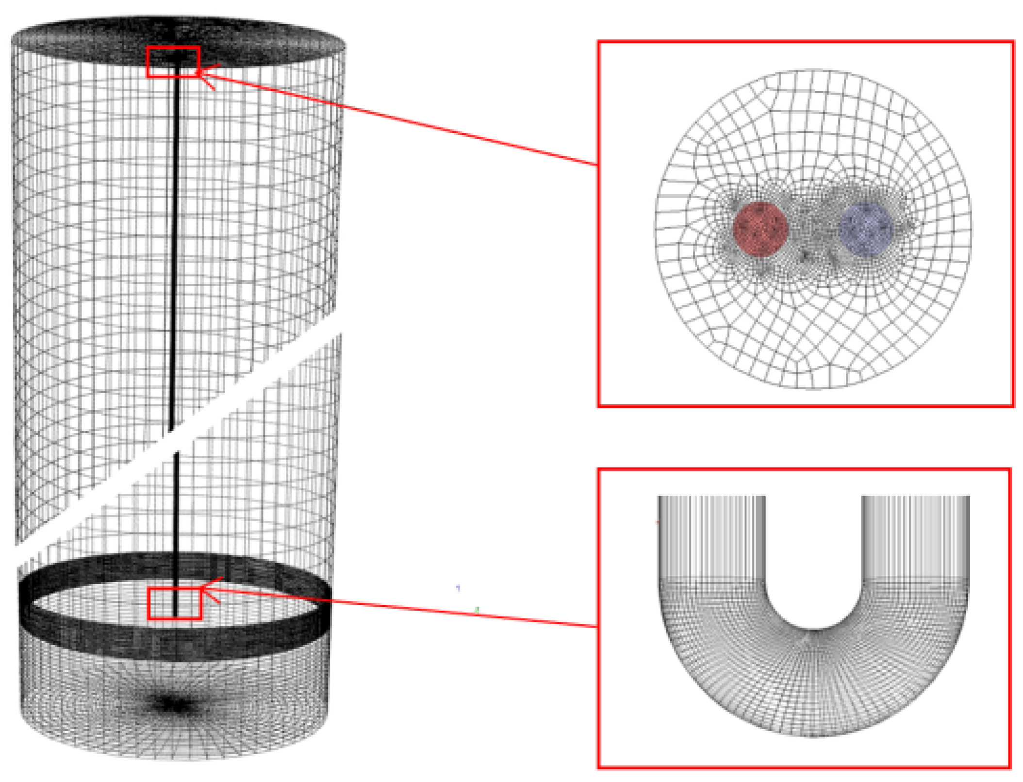
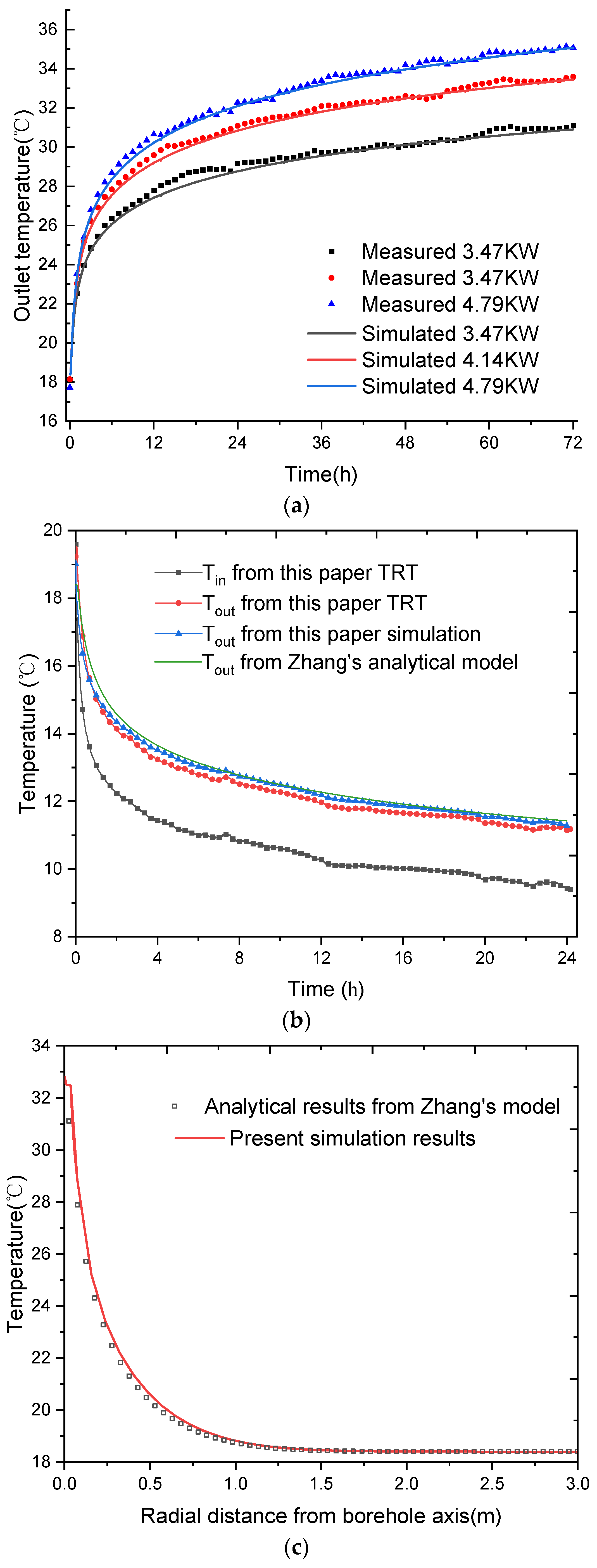
2. Model and Validation

To analyze the effect of precooling the ground, a vertical U-tube BHE model was developed by ANSYS 18.0 software. This model consisted of a heat carrier (water), a single U-tube heat exchanger, a geological medium backfill, and surrounding soil. Figure 1 shows the structure and detailed meshes.
The detailed design parameters were set according to the measured data, which are listed in Table 1. The physical parameters of the materials are shown in Table 2. The assumptions in this 3D transient heat transfer model were: the material properties of the water, the U-tube, the backfill material, and the soil do not vary with temperature; we ignored the impact of outdoor air temperature fluctuations on soil surface temperature. Moreover, Fan et al. [6] found that due to the existence of groundwater flow, it will move the cold energy charged to the soil using the BHE into the downstream zone, which is not conducive to cold energy storage. Similarly, the effect of precooling might be sharply decreased in the presence of groundwater flow. Therefore, we assumed that the underground area was approximated to a homogeneous field without an underground water flow. The boundary conditions are shown in Table 3.
The numerical model of the GHE was compared with the experimental data from Zhou et al. [20] and the thermal response test (TRT) experiment constructed in this research. The TRT experiment was constructed in the laboratory of the ground source heat pump in Donghua University. The inlet velocity and inlet temperature of the simulated working condition were set to the same the experimental data. To make a further validation about the thermal radius behaviour of the single U-tube BHE for the numerical model built in this research, an analytical solution developed by Zhang et al. [21] was introduced, which combined the transient moving finite line heat source (MFLS) model in the soil outside the BHE with the quasi-three-dimensional borehole thermal resistance model for the heat transfer inside the BHE. As shown in Figure 2, it was found that the results from the numerical model in this research agreed well with the results from Zhou et al. [20] and the TRT experimental data in this paper, respectively. As shown in Figure 2a, the maximum of relative error was 2%, 2%, and 4% when compared with the outlet temperature under three different heating power values of 4.79, 4.14, and 3.47 kW in a previous study [20]. As shown in Figure 2b, it was found that the trend of outlet temperature variation between the two methods was consistent, and the maximum error was 6%. As shown in Figure 2c, after 72 h of continuous operation for the tested inlet temperature of 35 °C, we compared radial soil temperature (at y = 0 m and z = 41 m) distribution in the simulated model and the Zhang’s analytical model [21]. It can be seen that the maximum error between the two methods was 4%.

3. Results and Analyses

In this study, precooling was used to give a lower soil temperature field before the start of the cooling season. Precooling refers to water continuously entering at 7 °C, flowing into the BHE for the cold energy injected into the soil. Then, water entering at 35 °C flows into the BHE (discharging) for cold energy extraction by the ground source heat pump system to meet the cooling load in buildings. We investigated how precooling and extended precooling impacted the improvement of the thermal radius in this study. The discharging process lasted for 7 days, during which the operation lasted for 12 h with the heat pump shutting down for 12 h every day. One was the no-precooling mode (Case 1); another four different precooling times were set before the start of the discharging process, including the precooling 3 d mode (Case 2), the precooling 7 d mode (Case 3), the precooling 14 d mode (Case 4), and the precooling 30 d mode (Case 5). A comparison of the different simulation cases is discussed in this section. The soil’s physical properties and related parameters were as mentioned above. Then, we focused on clarifying the impact of precooling and extended precooling on soil temperature and the thermal radius during the discharging process.

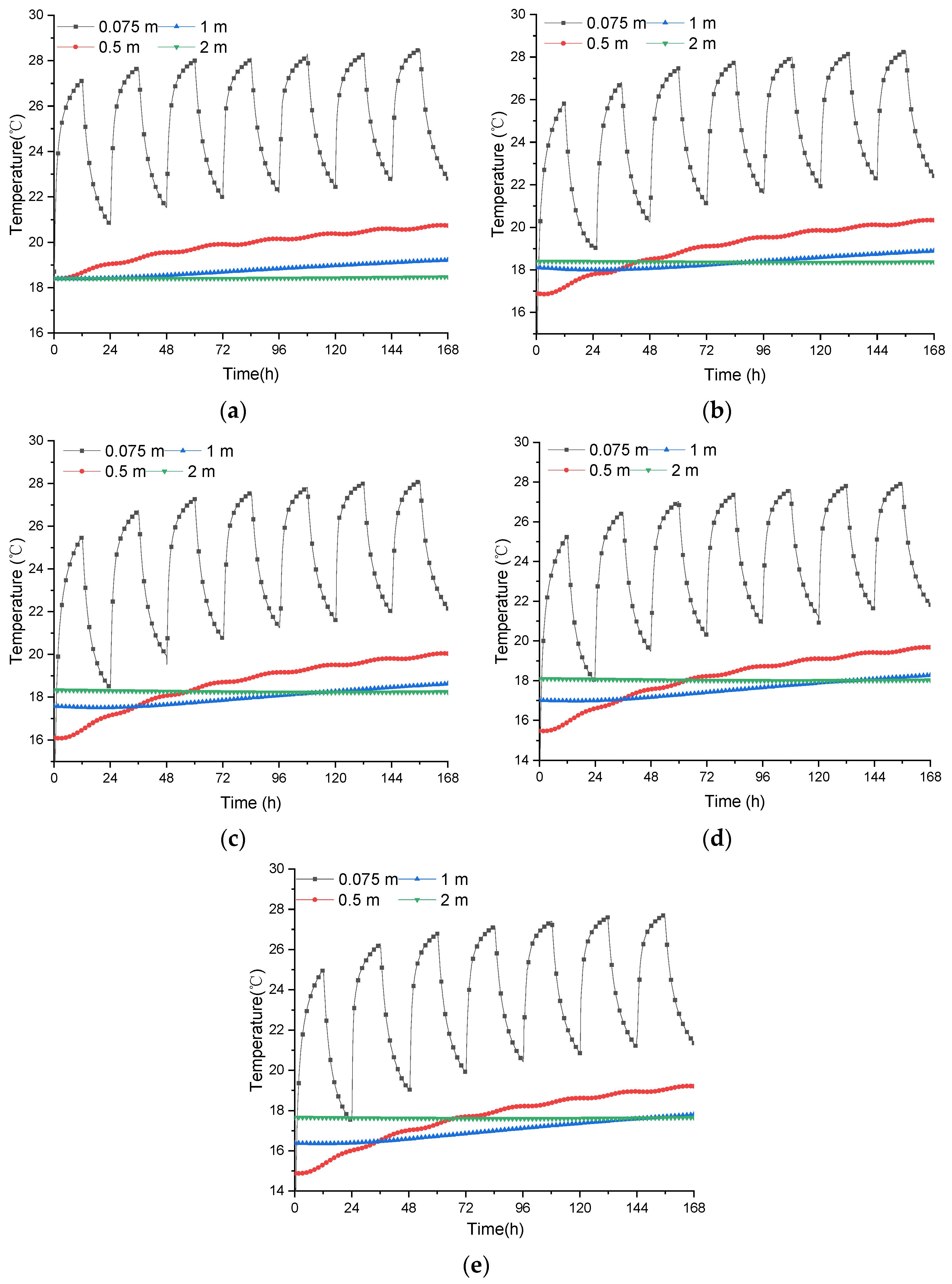
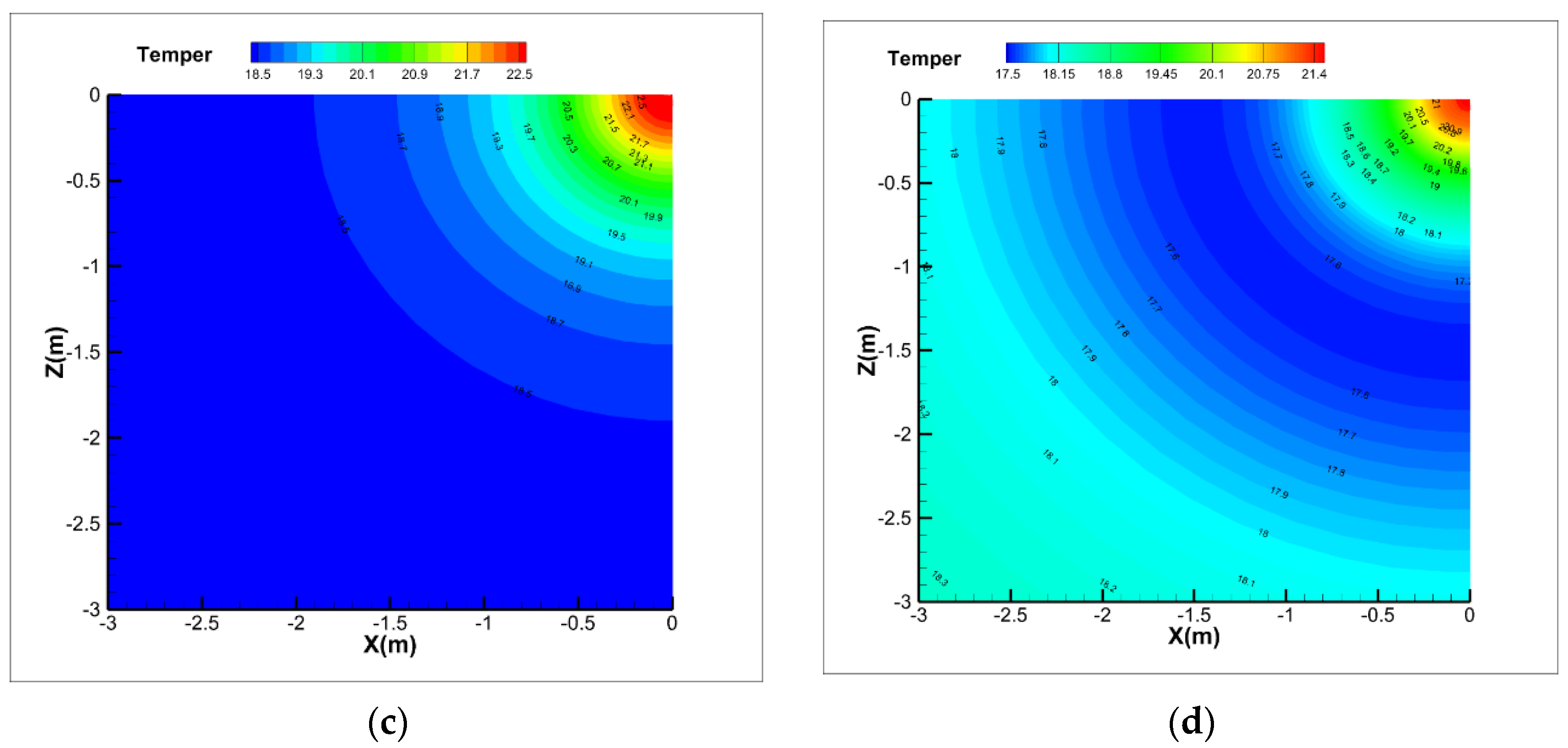
3.1. The Influence of Precooling Time on the Dynamic Soil Temperature

Without precooling, the soil temperature field was considered to be basically uniform at the beginning of the discharging process, which was equal to the initial soil temperature; precooling decreased the soil temperature to a greater extent, which was the same as the soil temperature at the end of the precooling period.
Figure 3 shows the distribution of soil temperature at the beginning of the discharging process under different precooling times. It can be seen that the lower soil temperature can be obtained when the precooling time is extended. Figure 4 shows the dynamic trend of the surrounding soil temperatures under different precooling times at the center cross-section of a 41 m depth (half depth of the borehole) at four different distances from U-tube pipes for a 168 h discharging process. The distances are with the magnitudes of 0.075 m, 0.5 m, 1 m, and 2 m from the BHE.
The excess temperature θ represents the soil temperature differences between a certain time and initial time for each monitoring point in the soil. Equation (1) for this calculation is as follows:
θ ( t ) = T s ( t ) T 0
where T s ( t ) is the temperature of the soil at a certain time, °C, and T 0 is the initial temperature of the soil, 18.4 °C.
As shown in Figure 4, in the mode without precooling (Case 1), the soil temperatures at the operation time of 168 h were 22.81, 20.74, and 19.22 °C at the borehole wall (r = 0.075 m) and in the soil at radial distances of 0.5 and 1 m from the borehole axis, respectively; the corresponding values were 4.41, 2.34, and 0.82 °C for the θ at the borehole wall and at radial distances of 0.5 and 1 m from the borehole axis, respectively. In the mode with precooling for 30 d (Case 5), the soil temperatures at the operation time of 168 h were 21.36, 19.21, and 17.79 °C at the borehole wall and in the soil at radial distances of 0.5 and 1 m from the borehole axis, respectively; the corresponding values were 2.96, 0.81, and −0.61 °C for the θ at the borehole wall and at radial distances of 0.5 and 1 m from the borehole axis, respectively. At the same time, the soil temperatures at a radial distance of 2 m in Case 1 and Case 5 were nearly equal to 18.47 and 17.66 °C. A comparative analysis of cases with and without precooling during the discharging process showed that Case 1 and Case 5 had a similar trend on the whole; the soil temperature change was more intense near the BHE than away from the BHE. In the radial direction of BHE (0.075 m), there was a rapid change. Compared with Case 1, Case 5 had a lower soil temperature, and Case 5 had a faster rise in soil temperature within the thermal radius range at each monitoring point due to the greater temperature difference between the BHE and soil temperature.
Figure 5 compares the soil temperature (at the center cross-section of a 41 m depth) field in Case 1 and Case 5 at the end of the operation and recovery period (the 156th and 168th hour) on the seventh day during the discharging process, respectively. It can be seen that the soil temperature around the BHE with precooling was still lower than that without precooling at the end of the discharging process. This suggests that precooling can improve the thermal efficiency of the BHE. As shown in Figure 5a,b, the soil temperature at the end of the discharging period increased due to the amount of thermal energy released within thermal radius zone. Figure 5c,d shows that the temperature decreased at the end of the recovery period.

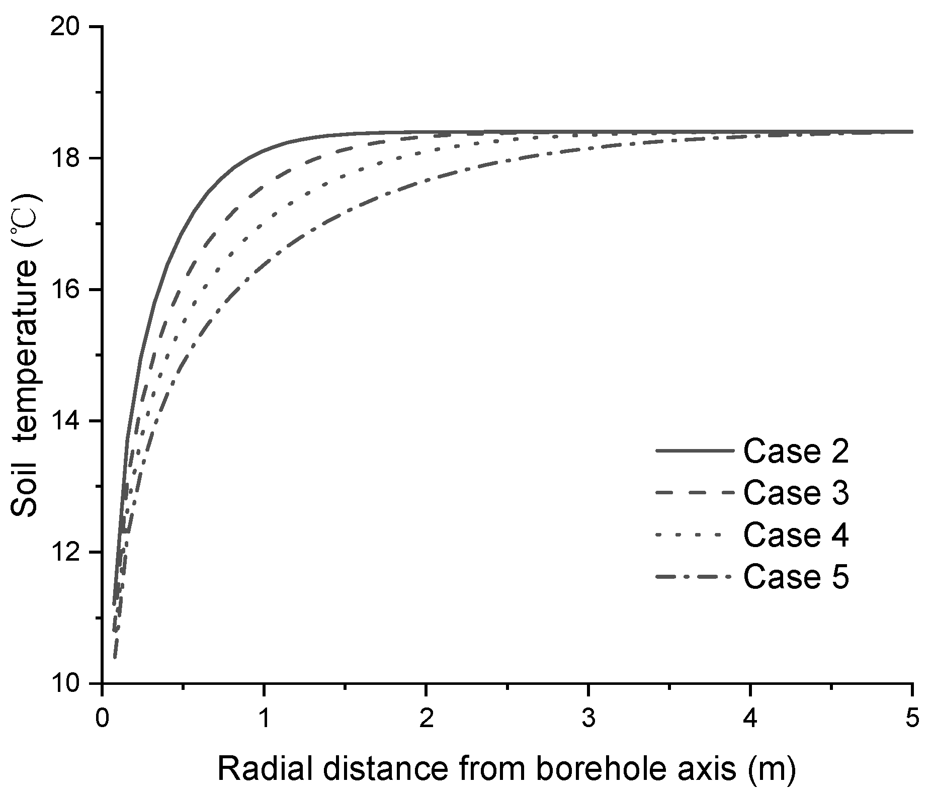
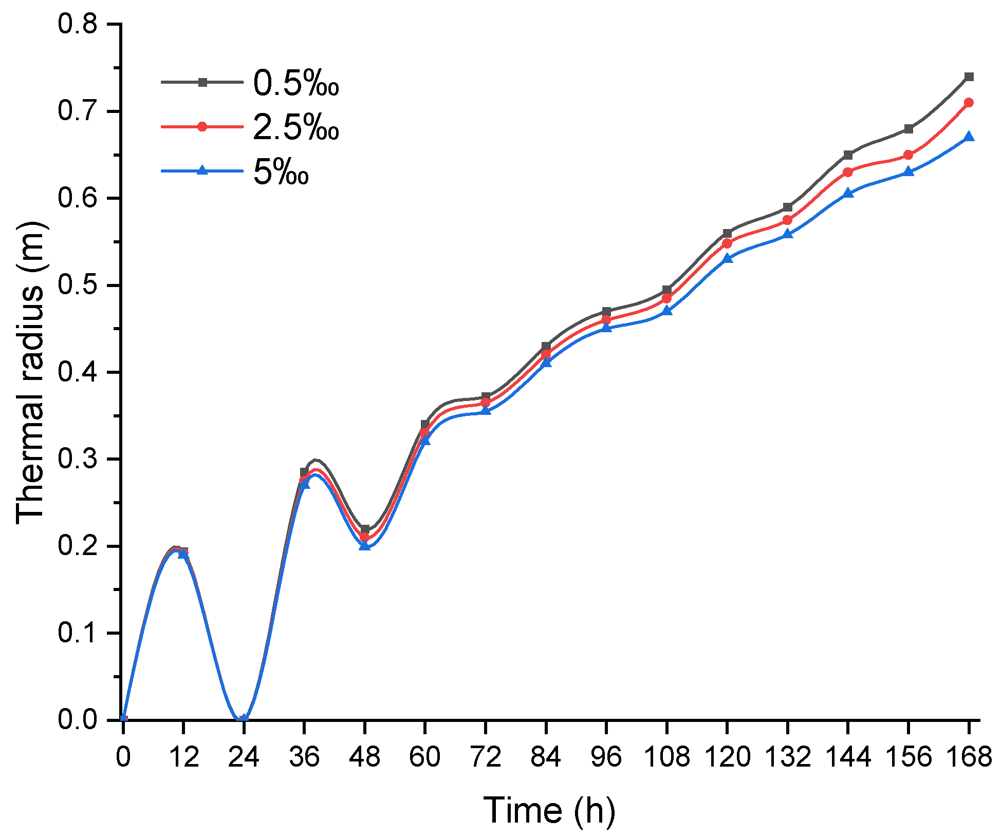
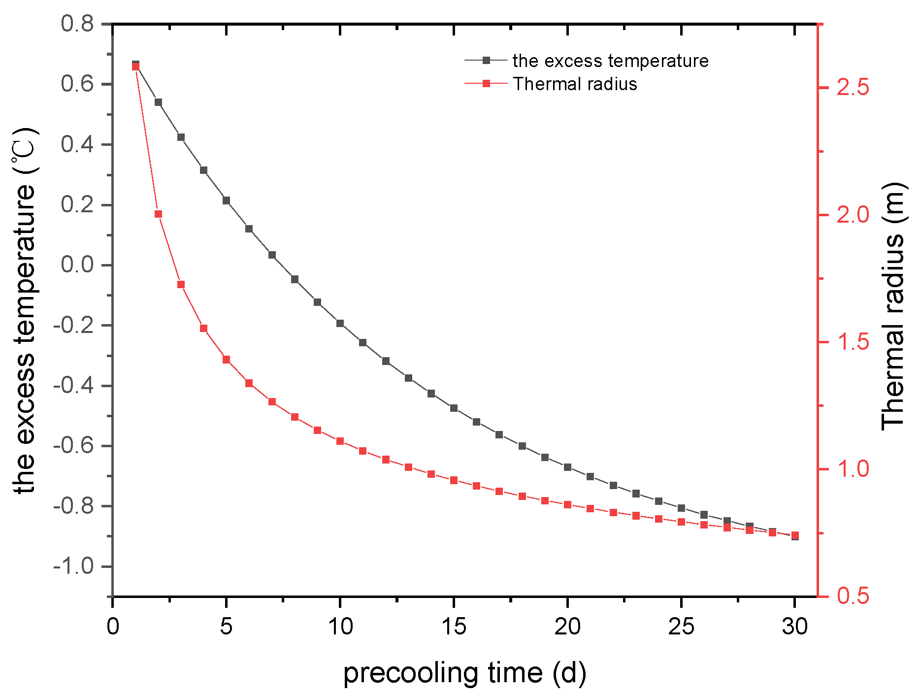
3.2. The Influence of Precooling Time on Thermal Radius

Hart and Couvilison [22], based on the Kelvin line source theory [23], proposed the concept of far-field radius and defined it as r = 4 a τ , which depends on the duration of the operation time and the thermal diffusivity of the soil. It is suitable for the case without precooling in which the soil temperature field was considered to be basically uniform at the beginning of the cooling condition and was equal to the initial soil temperature, but after precooling, the soil temperature decreased to a greater extent and was the same as the soil temperature at the end of recharging cold energy. The far-field radius formula described above needs further verification. In this paper, the variation thermal radius during the discharging process after precooling was studied. Although the thermal radius can be extended to infinity over time in theory, the excess temperature caused by it decays exponentially along the increase of distance in radial direction. When it decays to small enough, it can be approximately considered that all the heat dissipated by the BHE is absorbed by the soil within the corresponding distance, where it can be considered as the thermal radius. Therefore, compared with the initial temperature of the soil, the distance where the soil temperature change increased by 2.5‰ can be defined as the thermal radius ( r thermal ), which can be calculated as in Equation (2):
T s ( t ) T 0 T 0 = 2.5 s ( t ) = r thermal
When the initial soil temperature T 0 is 18.4 ℃, T s ( t ) T 0 = 0.046   .
To evaluate the accuracy of the indicator of 2.5‰ for determining the thermal radius, the sensitivity analysis about a range from 0.5‰ to 5‰ were conducted in the simulated Case 5, as illustrated in Figure 6. It can be seen that the indicator of 0.5‰, 2.5‰ and 5‰ for determining the thermal radius yields approximately the same results at the early stage. As time goes by, the thermal radius of using the indicator of 0.5‰ is the biggest, while that of the indicator of 5‰ is the smallest. It is obvious that the deviation between the results of the indicator of 0.5‰ and 5‰ are within the range of ±10%. As a compromise, the indicator of 2.5‰ for determining the thermal radius was then employed for the following calculations.
According to Equation (2), the hourly soil temperature value of each grid node around the BHE was derived from the ANSYS software, and then the thermal radius and the area-weighted average soil temperatures within the thermal radius are calculated.
Figure 7 shows the change in average soil excess temperature and thermal radius at the end of the 168 h discharging process under different precooling times. It can be seen that as the precooling time increased, the change rate of average soil excess temperature and thermal radius decreased, becoming smaller to different extents. The decreasing rate of the thermal radius became no more than 4% when the precooling time was longer than 10 days. For example, when the precooling time was from day 1 to day 10, the thermal radius decreased from 2.58 to 1.12 m, and the corresponding values were from 1.12 to 0.86 m from day 10 to day 20. The thermal radius difference of the former and latter was 1.46 and 0.26 m, respectively.
The change in the thermal radius zone under different precooling times was calculated as shown in Figure 8. It can be seen that the mode without precooling (Case 1) had a similar trend to that of Equation (2) for the thermal radius, which suggests that the equation is suitable for the intermittent operation conditions with a constant inlet temperature and variable heat flow boundary. Although the thermal radius kept increasing with the increase in the operating time, the increase in the degree decreased. However, Figure 8 shows that this equation was obviously not suitable for the mode with the precooling time including 3, 7, 14, and 30 d (Case 2, Case 3, Case 4, and Case 5). Compared to Case 1, the thermal radius in the mode with precooling fluctuated in the early stage and was smaller than that in Case 1. Furthermore, the thermal radius decreased as the precooling time increased. For example, the thermal radii at the end of 168 h of operation were 2.63, 1.72, 1.22, 0.92, and 0.71 m in Case 1, Case 2, Case 3, Case 4, and Case 5, respectively.
In order to provide more detail about the variation laws of the thermal radius in the mode without and with precooling, it was necessary to analyze the soil excess temperature distribution at the end of 12 h and 24 h under different precooling times, as shown in Figure 9. It can be seen that the soil excess temperature distribution in Case 1 had the exponential form of the temperature profile, but the mode with precooling was initially the exponential and then the logarithm form of the temperature profile. This was mainly because the longer the precooling time, the greater the injection of cooling energy, and thus the lower the soil temperature and the smaller the thermal radius. Figure 9a shows that the soil excess temperature’s degree increase decreased with the discharging time. For example, at 12 h, which was the end of the operation period on the first day, the soil excess temperature at the borehole wall decreased from 7.5 to 7.15 °C in Case 2 and Case 3, and the corresponding values were from 6.89 to 6.64 °C in Case 4 and Case 5. The temperature difference of the former and latter was 0.35 °C and 0.25 °C, respectively. Figure 9b shows that the soil excess temperature recovery degree increased with the precooling time. For example, at 24 h, which was the end of recovery period on the first day, the soil excess temperature at the borehole wall was 2.37 °C in Case 1, and the corresponding values were, respectively, 0.65, 0.07, −0.4, and −0.95 °C in Case 2, Case 3, Case 4, and Case 5.

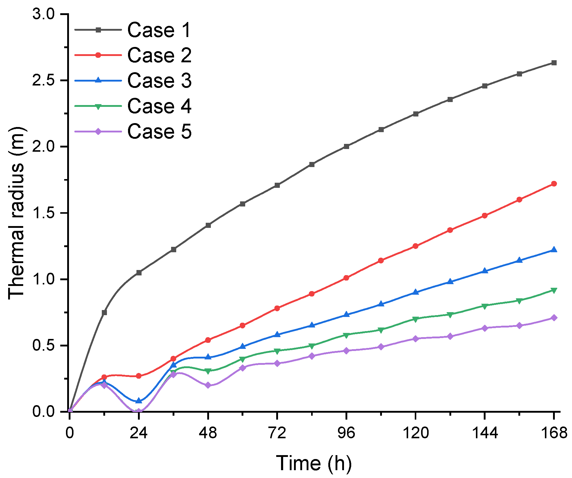
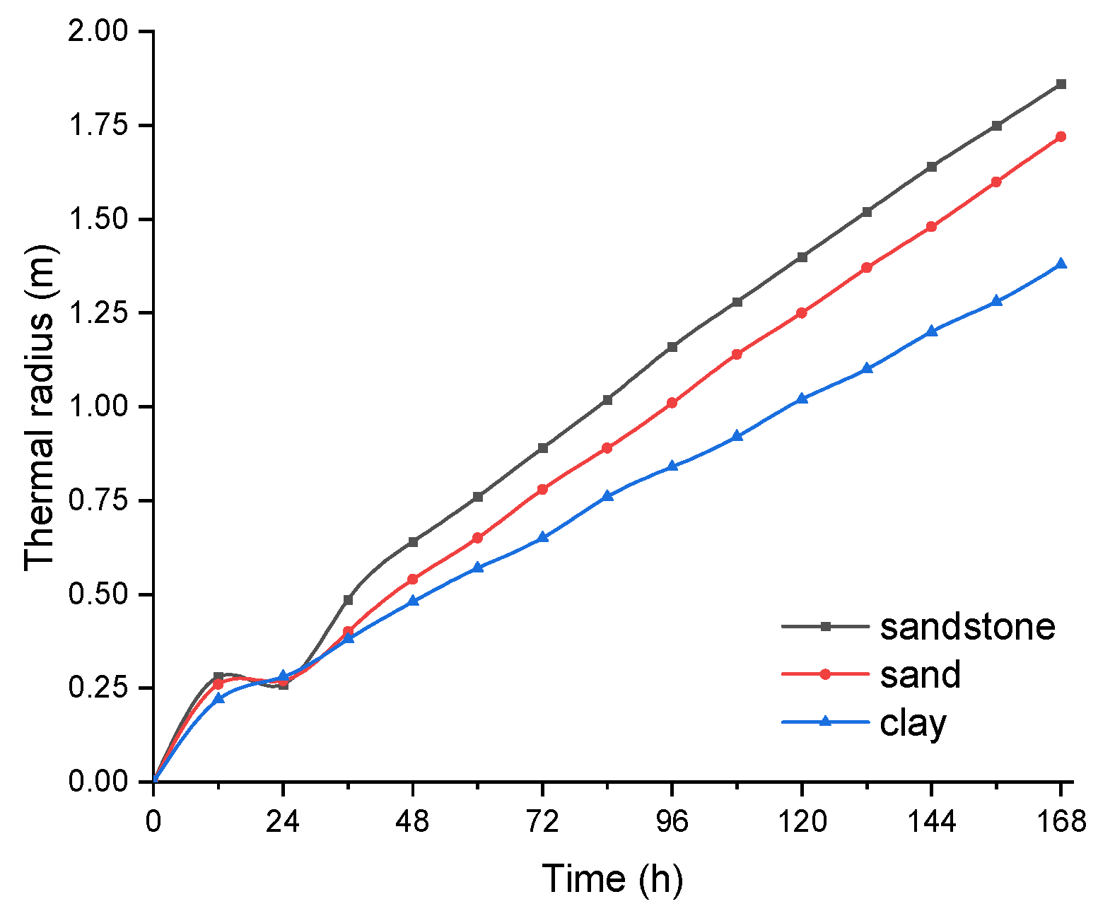
3.3. The Influence of Soil Type on Thermal Radius

The change in the soil type strongly affected the thermal properties of the soil and therefore influenced the thermal radius of the BHE. For the effects of soil type on thermal radius during the 168 h discharging process, the detailed thermophysical properties of three kinds of typical soils, including clay (Zhou et al., 2016) [24], sand (the TRT experiment), and sandstone (Li et al., 2018) [25], are given in Table 4. The simulated results are shown in Figure 10.
Three kinds of soils were in the mode with precooling for 3 d. Figure 10 shows the thermal radius with time under the three kinds of soil types. The thermal radius zones of clay, sand, and sandstone at the end of 168 h were 1.38, 1.72, and 1.86 m, respectively. It can be concluded that in terms of reducing the radius of thermal interference, clay is the most advantageous. The main reason is that the thermal conductivity and thermal diffusivity of clay is the smallest; the heat released to the soil near the BHE cannot be diffused rapidly outward, and thus results in the smallest thermal radius; the thermal diffusivity of sandstone is the largest, resulting in the heat released near the BHE diffusing outward rapidly. Therefore, it is suggested that smaller thermal conductivity and thermal diffusivity of a soil is beneficial to suppress the thermal interference effects of BHEs.

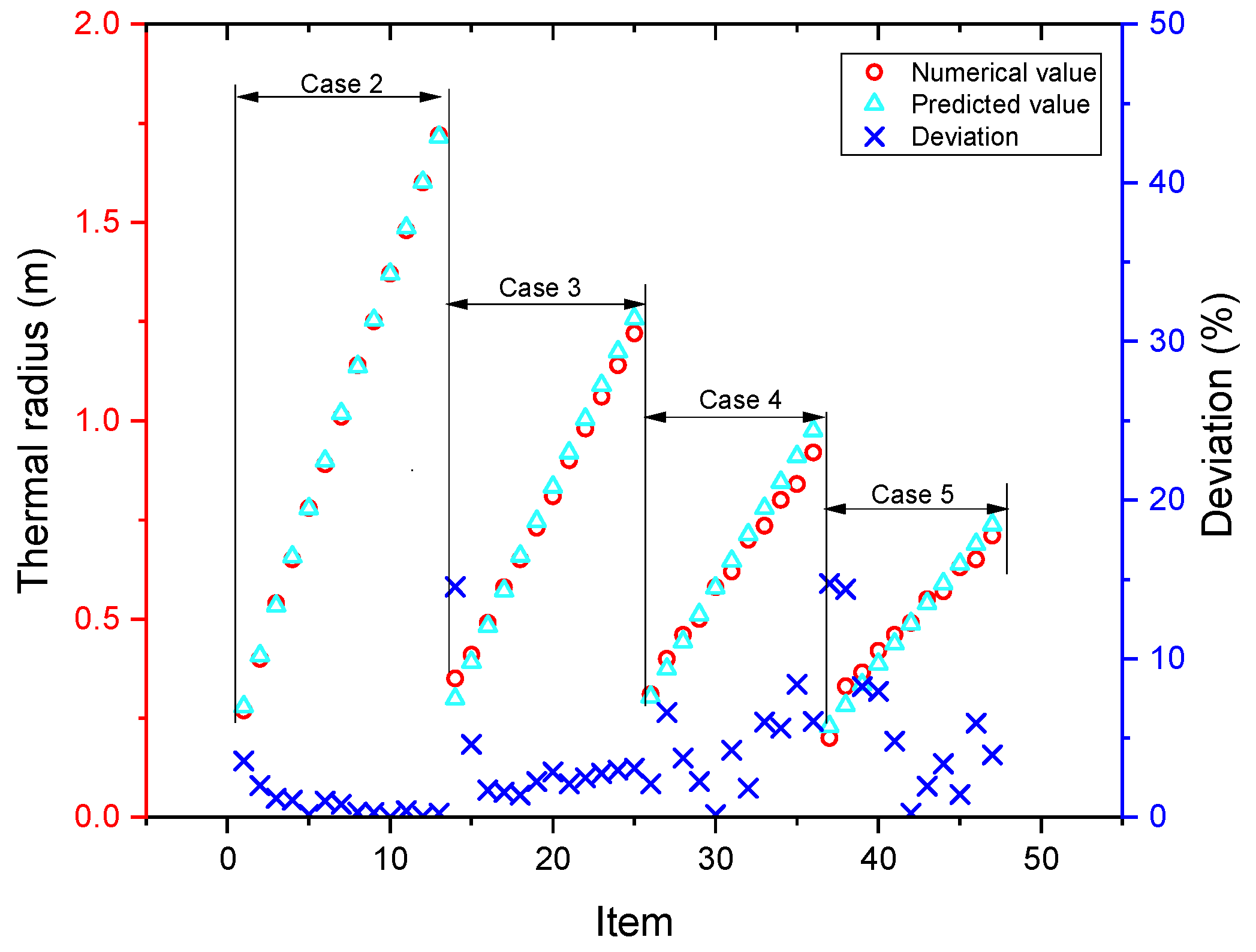
3.4. Numerical Formula for the Thermal Radius

The thermal radius ( r thermal ) of the BHE during the discharging process was subjected to regression analysis. Based on Figure 8 and Figure 10, we found three main factors affecting the thermal radius, which were thermal diffusivity (a, within the range of 0.42 × 10 6 · m 3 · s 1 ~ 1.08 × 10 6 · m 3 · s 1 ), precooling time ( τ 1 , within the range of 0~30 day), and discharging time ( τ 2 , within the range of 0~7 day). Therefore, there was one dependent variable and three independent variables in the regression analysis. The nonlinear relationship between the dependent variable and the independent variables is essential, which belongs to the multivariate nonlinear regression analysis [26,27]. We initially assumed a power function for the regression model, as defined by Equation (3):
r thermal = β 0 τ 1 β 1 τ 2 β 2 a β 3
where: r thermal —thermal radius, m; a—thermal diffusivity, m2/s; τ 1 —precooling time, s; τ 2 —discharging time, s.
We took the logarithm of both sides to obtain:
ln r thermal = ln β 0 + β 1 ln τ 1 + β 2 ln τ 2 + β 3 ln a
Using ln r thermal as the dependent variable, ln τ 1 , ln τ 2 , and ln a as the independent variables, a multiple linear regression fitting was used. The results are shown in Table 5. Equation (6) shows the empirical correlation of the thermal radius, which was decided by thermal diffusivity; precooling time and discharging time can be obtained when the multiple nonlinear regression analysis was performed.
ln r thermal = 3.06761 0.36646 ln τ 1 + 0.932308 ln τ 2 + 0.301736 ln a
r thermal = EXP ( 3.06761 ) τ 1 0.36646 τ 2 0.932308 a 0.301736
Table 5 shows that the coefficient of determination in the model was 0.944948, and the significance sig was 4.21 × 10−42, indicating that the correlation between the dependent variable and the independent variable after regression was high and the fitting effect was good.
In order to test the regression prediction model, the simulated values and the predicted values of the thermal radius in the mode with four different precooling times, including 3, 7, 14, and 30 d (Case 2, Case 3, Case 4, and Case 5), were compared with the predicted values for the sandy soil, as shown in Figure 11, and the regression prediction formula shows that the calculated results were in good agreement with the simulated calculation results, and the deviation was not more than 14.8%.

4. Conclusions

In this work, a numerical study on the effects of precooling the ground to improve the performance of GSHP was investigated. For this purpose, Ansys 18.0 software was extended to a BHE in a fully coupled three-dimensional model. The model result was compared to experimental data, indicating that the maximum error of the outlet temperature was 6% and ensuring correct implementation. This extended feature allowed the simulation of a model with four different precooling times, which included 3, 7, 14, and 30 d, and then we evaluated the influence of the precooling time on two key operation characteristic parameters during the discharging process: soil temperature and the thermal radius ( r thermal ). To further obtain the effects of soil type on thermal radius ( r thermal ) of the BHE, three kinds of typical soils were chosen, and the following conclusions can be drawn:
(1). The quantitative comparison of the soil temperature response to the intermittent discharging process with and without precooling. The result showed that, the soil temperature increased more with precooling, but the soil temperature was lower than the case without precooling. However, when the precooling time was longer than 14 days, the thermal radius rate percentages decline less than 4%.
(2). The analysis of the three soil types showed that sandstone had the largest thermal conductivity and thermal diffusivity, followed by sand and clay. It was demonstrated that clay is the most advantageous from the perspective of thermal interference. Therefore, this suggests that a lower thermal conductivity and thermal diffusivity of soil is beneficial for suppressing the thermal interference effects of BHEs.
(3). The thermal radius with and without precooling is different. There was a characteristic in that the thermal radius with precooling fluctuated in the initial stage and was smaller than without precooling. The numerical expressions of the thermal radius comprehensively considered the effects of the thermal diffusivity; the precooling time and discharging time were fitted, and the prediction deviation was within 14.8%.

Author Contributions

Conceptualization, S.Z. and J.S.; methodology, S.Z. and J.S.; software, S.Z. and J.S.; formal analysis, S.Z., J.S., K.Z. and H.C.; writing—original draft preparation, S.Z. and J.S.; writing—review and editing, S.Z., J.S., K.Z. and H.C.; project administration, S.Z. All authors have read and agreed to the published version of the manuscript.

Funding

This research received no external funding.

Institutional Review Board Statement

Not applicable.

Informed Consent Statement

Not applicable.

Data Availability Statement

Not applicable.

Conflicts of Interest

The authors declare no conflict of interest.

References

  1. Xu, L.; Pu, L.; Zhang, S.; Li, Y. Hybrid ground source heat pump system for overcoming soil thermal imbalance: A review. Sustain. Energy Technol. Assess. 2021, 44, 101098. [Google Scholar] [CrossRef]
  2. Zhang, J.; Zhang, H.-H.; He, Y.-L.; Tao, W.-Q. A comprehensive review on advances and applications of industrial heat pumps based on the practices in China. Appl. Energy 2016, 178, 800–825. [Google Scholar] [CrossRef]
  3. Xi, J.; Li, Y.; Liu, M.; Wang, R.Z. Study on the thermal effect of the ground heat exchanger of GSHP in the eastern China area. Energy 2017, 141, 56–65. [Google Scholar] [CrossRef]
  4. Abbas, Z.; Chen, D.; Li, Y.; Yong, L.; Wang, R.Z. Experimental investigation of underground seasonal cold energy storage using borehole heat exchangers based on laboratory scale sandbox. Geothermics 2020, 87, 101837. [Google Scholar] [CrossRef]
  5. Fan, R.; Jiang, Y.; Yao, Y.; Ma, Z. Theoretical study on the performance of an integrated ground-source heat pump system in a whole year. Energy 2008, 33, 1671–1679. [Google Scholar] [CrossRef]
  6. Fan, R.; Jiang, Y.; Yao, Y.; Shiming, D.; Ma, Z. A study on the performance of a geothermal heat exchanger under coupled heat conduction and groundwater advection. Energy 2007, 32, 2199–2209. [Google Scholar] [CrossRef]
  7. Yang, T.; Zhang, X.; Zhou, B.; Zheng, M. Simulation and experimental validation of soil cool storage with seasonal natural energy. Energy Build. 2013, 63, 98–107. [Google Scholar] [CrossRef]
  8. Yu, Y.; Ma, Z.; Li, X. A new integrated system with cooling storage in soil and ground-coupled heat pump. Appl. Therm. Eng. 2008, 28, 1450–1462. [Google Scholar] [CrossRef]
  9. Sagia, Z.; Rakopoulos, C.; Kakaras, E. Cooling dominated hybrid ground source heat pump system application. Appl. Energy 2012, 94, 41–47. [Google Scholar] [CrossRef]
  10. Pertzborn, A.J.A.T. Thermal storage properties of a hybrid ground source heat pump. ASHRAE Trans. 2012, 118, 34. [Google Scholar]
  11. Pertzborn, A.J. An Examination of Control Strategies in a HyGSHP System. In International High Performance Buildings Conference; Purdue University: West Lafayette, IN, USA, 2012; Available online: http://docs.lib.purdue.edu/ihpbc/61 (accessed on 10 November 2021).
  12. Pertzborn, A.J.; Nellis, G.F.; Klein, S.A. An evaluation of the effectiveness of pre-cooling in hybrid ground source heat pump systems. Proc. SimBuild 2012, 5, 144–151. [Google Scholar]
  13. Johansson, E. Optimization of Ground Source Cooling Combined with Free Cooling for Protected Sites. Master’s Thesis, Department of Applied Thermodynamics and Refrigeratio, KTH School of Industrial Engineering and Management, Stockholm, Sweden, 2012. [Google Scholar]
  14. Hackel, S.; Pertzborn, A. Effective design and operation of hybrid ground-source heat pumps: Three case studies. Energy Build. 2011, 43, 3497–3504. [Google Scholar] [CrossRef]
  15. Zhou, S.; Cui, W.; Li, Z.; Liu, X. Feasibility study on two schemes for alleviating the underground heat accumulation of the ground source heat pump. Sustain. Cities Soc. 2016, 24, 1–9. [Google Scholar] [CrossRef]
  16. Alaica, A.A.; Dworkin, S.B. Characterizing the effect of an off-peak ground pre-cool control strategy on hybrid ground source heat pump systems. Energy Build. 2017, 137, 46–59. [Google Scholar] [CrossRef]
  17. Yi, M.; Hongxing, Y.; Zhaohong, F. Study on hybrid ground-coupled heat pump systems. Energy Build. 2008, 40, 2028–2036. [Google Scholar] [CrossRef]
  18. Fan, R.; Gao, Y.; Hua, L.; Deng, X.; Shi, J. Thermal performance and operation strategy optimization for a practical hybrid ground-source heat-pump system. Energy Build. 2014, 78, 238–247. [Google Scholar] [CrossRef]
  19. Yang, W.; Zhang, H.; Liang, X. Experimental performance evaluation and parametric study of a solar-ground source heat pump system operated in heating modes. Energy 2018, 149, 173–189. [Google Scholar] [CrossRef]
  20. Zhou, Y.; Zhao, L.; Wang, S. Determination and analysis of parameters for an in-situ thermal response test. Energy Build. 2017, 149, 151–159. [Google Scholar] [CrossRef]
  21. Zhang, C.; Chen, P.; Liu, Y.; Sun, S.; Peng, D. An improved evaluation method for thermal performance of borehole heat exchanger. Renew. Energy 2014, 77, 142–151. [Google Scholar] [CrossRef]
  22. Hart, D.P.; Couvillion, R. Earth Coupled Heat Transfer; Publication of National Water Well Association: Dublin, Ireland, 1986. [Google Scholar]
  23. Kelvin, S.; Thomson, W. Mathematical and Physical Papers, 2nd ed.; Cambridge University Press: Cambridge, UK, 1882; Volume 2, p. 41. [Google Scholar]
  24. Zhou, S.; Cui, W.; Tao, J.; Peng, Q. Study on ground temperature response of multilayer stratums under operation of ground-source heat pump. Appl. Therm. Eng. 2016, 101, 173–182. [Google Scholar] [CrossRef]
  25. Li, W.; Li, X.; Peng, Y.; Wang, Y.; Tu, J. Experimental and numerical investigations on heat transfer in stratified subsurface materials. Appl. Therm. Eng. 2018, 135, 228–237. [Google Scholar] [CrossRef]
  26. Zhong, K.; Wang, Y.; Pei, J.; Tang, S.; Han, Z. Super efficiency SBM-DEA and neural network for performance evaluation. Inf. Process. Manag. 2021, 58, 102728. [Google Scholar] [CrossRef]
  27. Zhong, K.; Li, C.; Wang, Q. Evaluation of bank innovation efficiency with data envelopment analysis: From the perspective of uncovering the black box between input and output. Mathematics 2021, 9, 3318. [Google Scholar] [CrossRef]
Figure 1. Geometry and its mesh for the numerical simulations.
Energies 15 00151 g001
Figure 2. (a): Comparison between the results from the simulative model built in this research and experimental data from Zhou et al. [20]. (b): The simulative model built in this research was compared with the results from TRT experimental data and Zhang’s model [21]. (c): Comparison of the radial soil temperature (at y = 0 m and z = 41 m) from the simulative model built in this research and the analytical solution from Zhang’s model [21].
Energies 15 00151 g002
Figure 3. The distribution of soil temperature at the beginning of the discharging process under different precooling times.
Energies 15 00151 g003
Figure 4. Dynamic temperature response at the borehole wall (r = 0.075 m) and in the soil at radial distances of 0.5, 1, and 2 m from the borehole axis under different precooling times. (a) Without precooling (Case 1); (b) With precooling 3 d (Case 2); (c) With precooling 7 d (Case 3); (d) With precooling 14 d (Case 4); (e) With precooling 30 d (Case 5).
Energies 15 00151 g004
Figure 5. The simulation results of the soil temperature (at the center cross-section of 41 m depth) field at the end of the operation and recovery period during the discharging process with and without precooling, respectively. (a) Operation period end without precooling (Case 1); (b) Operation period end with precooling (Case 5); (c) Recovery period end without precooling (Case 1); (d) Recovery period end with precooling (Case 5).
Energies 15 00151 g005aEnergies 15 00151 g005b
Figure 6. The indicator for determining the thermal radius sensitivity analysis results.
Energies 15 00151 g006
Figure 7. Variation in average soil excess temperature and thermal radius at the end of the 168 h discharging process under different precooling times.
Energies 15 00151 g007
Figure 8. Variation in thermal radius with time under different precooling times.
Energies 15 00151 g008
Figure 9. The distribution of soil excess temperature at the end of the operation and recovery period (at 12 h and 24 h) on the first day during the discharging process under different precooling times. (a) Operation period end; (b) Recovery period end.
Energies 15 00151 g009
Figure 10. Variation in thermal radius with time under three kinds of soil types.
Energies 15 00151 g010
Figure 11. Comparison of simulated and predicted thermal radius.
Energies 15 00151 g011
Table 1. Design parameters for the numerical model.
ParametersValue
Boreholes depth (m)82
Pipe outer diameter (m)0.032
Pipe wall thickness (m)0.003
Legs center distance (m)0.07
Borehole diameter (m)0.15
Inlet velocity (m/s)0.7
Inlet temperature for cool charged (°C)7
Inlet temperature for cool discharged (°C)35
Initial soil temperature (°C)18.4
Table 2. The physical parameters of the materials.
ItemDensity/Thermal Conductivity/Specific Heat Capacity/
kg · m 3 W · ( m · ) 1 J · ( kg · ) 1
soil (sand)17902.11465
Backfill material22662.31731
HDPE11000.461450
water998.20.64182
Table 3. Boundary and simulation conditions.
TermsConditions
Inlet of U-tubeTinlet = 7/35 °C; vinlet = 0.7 m/s
Outlet of U-tubePressure outlet
Top and bottom boundaries of backfillingNo-slip wall with heat flux = 0 W/m2
Soil zone Faraway boundaryNo-slip wall with Dirichlet condition (T = 18.4 °C)
Table 4. Thermophysical parameters for three kinds of soils.
TypeDensitySpecific Heat CapacityThermal ConductivityThermal Diffusivity
kg · m 3 W · ( m · ) 1 J · ( kg · ) 1 × 10 6 · m 3 · s 1
Clay143014390.8620.42
Sand179014652.10.8
Sandstone259210652.981.08
Table 5. Regression analysis results.
Coefficients p-ValueSignificance FR Square
ln β 0 −3.0676130.00150094.2053 × 10−420.9449479
β 1 −0.3664636.322 × 10−30
β 2 0.93230771.591 × 10−39
β 3 0.3017365.492 × 10−7
Publisher’s Note: MDPI stays neutral with regard to jurisdictional claims in published maps and institutional affiliations.

