Abstract
As a consequence of the increasing share of renewable energies and sector coupling technologies, new approaches are needed for the study, planning, and control of modern energy systems. Such new structures may add extra stress to the electric grid, as is the case with heat pumps and electrical vehicles. Therefore, the optimal performance of the system must be estimated considering the constraints imposed by the different sectors. In this research, an energy system dispatch optimization model is employed. It includes an iterative approach for generating grid constraints, which is decoupled from the linear unit commitment problem. The dispatch of all energy carriers in the system is optimized while considering the physical electrical grid limits. From the considered scenarios, it was found that in a typical German neighborhood with 150 households, a PV penetration of ∼5 kWp per household can lead to curtailment of ∼60 MWh per year due to line loading. Furthermore, the proposed method eliminates grid violations due to the addition of new sectors and reduces the energy curtailment up to . With the optimization of the heat pump operation, an increase of of the self-consumption was achieved with similar results for the combination of battery systems and electrical vehicles. In conclusion, a safe and optimal operation of a complex energy system is fulfilled. Efficient control strategies and more accurate plant sizing could be derived from this work.
1. Introduction
1.1. Background
Nowadays, there are several initiatives and international efforts to reduce the CO emissions in all energy sectors as part of the Paris agreement [1]. In Germany, the so-called “Energiewende” establishes the goals for the energy transformation towards a zero-emission national energy system [2]. A fundamental step to achieve such ambitious goals is the electrification of the residential heat and transport sectors that accounted in 2016 for ∼10% and ∼18.2% of the total emissions in Germany, respectively [3]. By 2050, an increase of of the district heating in Europe is expected, with approximately of that demand being covered by heat pumps [4]. However, combined heat and power is expected to serve as a bridge technology coupling electricity and heat sectors [5]. Additionally, a fleet of around six million electrical vehicles is planned by the German government by 2030 [6]. This makes the analysis of modern and future energy systems more challenging, due to the added complexity of the new technologies and energy sectors. Along with a significant deployment of renewable sources in the electricity grid, the integration of these sector coupling technologies may add an extra burden to the existing distribution grids [7,8]. Therefore, new concepts and techniques are needed to properly study and optimize the grid structure for adequate operation of such new energy systems [9]. In this research, an approach that enables the ease evaluation and optimization of energy systems considering the power grid limits is developed. This methodology was based on the energy system for the “Energetisches Nachbarschaftsquartier Fliegerhorst Oldenburg”, which will be a living laboratory in the city of Oldenburg, Germany [10].
1.2. Optimization of Energy Systems
Typically, the aggregation approach has been of common use in the literature when it comes to the analysis and optimization of energy systems [11]. Then, the optimization problem is independent of its actual physical characteristics. Mathematically, the energy system optimization problem can be expressed as:
The Equation (1) minimizes the cost in a period T at a resolution . The set E represents the energy flow between nodes, whereas the set N represents the flows between nodes and sources. The sets to establish the alternative to have multiple flows with different associated costs. Fixed and time-varying costs are included in c. The variable p denotes the power that flows between nodes and sources. The set J constitutes the types of sectors to consider (e.g., heat and electricity), whereas the set M represents the demand associated with the sector. The inequality constraint (2) ensures that the sum of the M demands for each sector is fulfilled by the sum of the sources multiplied by the coupling factor a corresponding to the source and the sector. The constraints (3) and (4) represent the boundary conditions for flows and sources.
Many approaches are found in the literature dealing with the optimization of energy systems considering the actual electrical grid topology. For power systems, the implementation of linearized power flows approaches to relax the optimization problem is of common use in the researched literature [12,13]. Whereas the typical DC power flow neglects reactive power, some studies have enhanced the method by adding the consideration of reactive power and with the implementation of data-driven approaches to determine voltage magnitudes and angles [14]. Novoa et al. [15] have applied a decoupled linearized power flow [16] in combination with a mixed-integer linear problem to find the optimal allocation of PV and batteries within an energy system. However, these methods are less accurate than the AC power flow and more complex than the DC power flow. The combination of a commercial tool to solve power flow problems with a linear unit commitment is presented by Nolden et al [17]. In this approach, only an electrical system without storage at a single time step is considered. Similarly, Fortenbacher et al. [11] propose a distributed model predictive control within sub-grids to solve a multi-period dispatch optimization problem.
When an entire energy system with multiple energy carriers is optimized, generally the physical structures are disregarded and the systems are simplified. Some solutions to work around the over-simplification of the models have been developed. Lohmeier et al have proposed specialized tools for each energy sector that can be implemented together in a co-simulation [18]. As the physical constraints of the energy systems are considered, the complexity in solving such problems also increases. For instance, non-convex systems result when hydraulic equations are taken into consideration in an energy hub with multiple energy carriers [19]. The time-step dependency from energy storage may add extra complexity to the already mentioned systems. The utilization of the Newton–Rapson method is inefficient in time-domain equations. Therefore, Levron et al. [20] have used in combination with a power flow solver, dynamic programming to tackle the time-dependent functions. As the share of renewable energies increases at the medium and low voltage of the grid, some power quality issues such as line over-loading and over-voltages may appear [7,9]. For this reason, the potential of CHP and P2G options has been considered to provide grid flexibilization [21,22].
The main contribution of this research is the development of a decoupled approach for the dispatch optimization of a sector coupled energy system. The method takes into consideration the electric grid limits to optimally integrate different energy sectors into an energy system. In order to assess the method, some scenarios comprising an energy system with high share of renewables, storage systems, and sector coupling technologies were considered. As a main result, it was found that high shares of PV without storage lead to a higher energy curtailment. Additionally, the proposed method was capable of reducing energy curtailment and increase self-consumption of the energy system by adding flexibility through the implementation of heat pumps and electric vehicles.
2. Methodology
In this section, the implemented methodology to consider grid limitations in dispatch optimization problems in energy systems is presented. The idea behind this work is to reduce the complexity of the optimization problem when considering grid constraints. The unit commitment problem and the power flow solutions are decoupled, the solution to the unit commitment is realized considering a mixed-integer linear problem (MILP) using oemof-Solph [23], whereas an AC optimal power flow (OPF) calculation is carried out in PowerFactory [24] to verify grid quality standards compliance. From this OPF, grid congestion and voltage violations are avoided; the measurements to achieve this are re-implemented in the linear problem as constraints. Figure 1 shows this iterative process to obtain the solution of the optimization problem in the energy system. Even though this approach could be applied to any energy system, regardless of its dimension, this work is primarily intended for its implementation on mid and low voltage systems as described in Section 1.
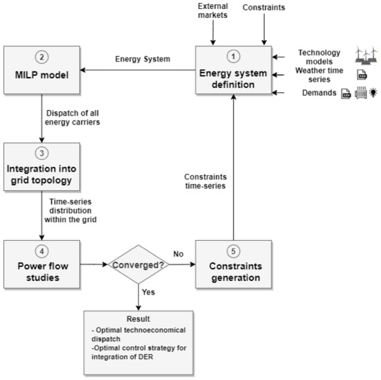
Figure 1.
Steps for constraints generation in the optimization process.
2.1. Overview: Iterative Process
Since sector coupling and energy storage technologies will be present in the energy systems of the future, an iterative approach is needed when decoupling the unit dispatch optimization and the grid constraint generation. This is due to the fact that the constraint generation from the OPF may influence the dispatch of the sector coupling technologies and storage such as heat pumps, heat water tank, and batteries.
This section presents an overview of the main steps depicted in Figure 1.
- Energy system structure: Here, the energy sectors to be considered are defined as well as the relevant technologies and their models. Natural renewable resources and demands time series must also be included. Time steps have to be big enough to make valid the steady-state assumption of the different energy sectors [18]. In this work, only the electric and heat sector are considered and a time step of an hour during a year is evaluated. Although several technologies, markets, and demands could be present in a distributed energy system [25], only the ones presented in Table 1 were considered in this study. Furthermore, the energy system is seen as a system aggregator from the grid perspective. This means that the system can buy and sell electricity in the market.
 Table 1. Summary of the considered energy system components.
 - Linear unit commit: Using a holistic approach, an abstraction of the energy system structure is created in oemof-Solph. This abstraction contains all possible energy flows between sources and sinks, and between energy sectors through the coupling technologies as depicted in Figure 2.
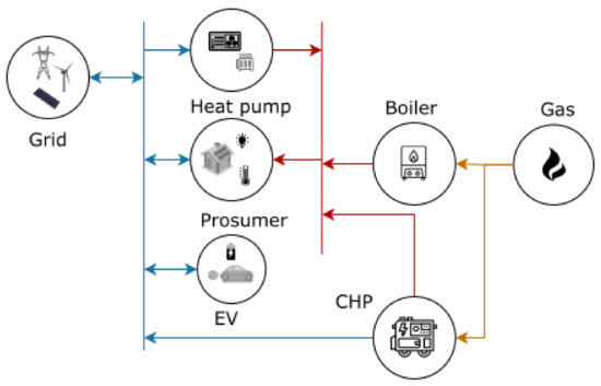 Figure 2. Simplified example of an energy system structure representation in oemof-Solph and the energy flow between sectors. The blue lines represent the electrical part of the system, whereas the red and orange represent the heat and gas sectors, respectively.Costs and additional constraints can be associated with each of the energy flows [23]. Here, the system will only consider the economical constraints of the energy flows. Therefore, the objective function is the cost minimization. From Equation (1), the following objective equation is derived for the considered energy system:where represents the imported or exported electric power from the external grid, the day ahead price for a given time, and the gas import for the CHP and boiler, respectively, and represents the cost of gas. The power given or provided to the external grid at a given time is given by . The electric generation and electric loads can be defined as follows:In Equations (7) and (8), the parameters and refer to the PV generation and the CHP electric power generation within the system, whereas the parameters , , , and refer to the electric demand, the battery power consumption, electrical vehicle charging, and the heat pump demand, respectively. Every storage unit (including EVs) has been considered as a load. That means that a negative power represents a power injection to the system. The same convention has been used for the external grid power flow. As constraints for the optimization problem, the thermal and electric demands must be supplied at any time. Equations (9) and (10) depict such constraints where , , and are fixed time series.As a result, the optimized power dispatch for each non-fixed source to supply the demand at each time step is obtained. However, up to this point, just the total installed capacities and demands have been considered as per the inequality (4). The actual topology of the electrical and thermal grid has been also disregarded as a common practice in the optimization of energy systems [19].
 - Grid topology consideration: Before integrating these flows into the electrical grid in PowerFactory, the flow distribution must be considered. This applies only to the electric sources, sinks, and sector coupling technologies. The distribution of heat technologies is disregarded since only the electrical grid topology is being considered in this study.To represent a typical low voltage grid, one of the so-called “Merit Order Netz-Ausbau 2030” (MONA) reference grids is used. The ONT_8003 grid model is used as reference [26] and depicted in Figure 3. This topology represents a typical low voltage grid in Germany.
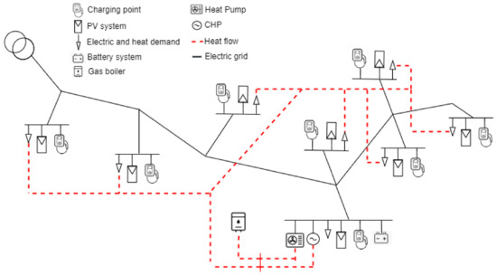 Figure 3. Representation of the ONT_8003 MONA grid with the addition of the technologies mentioned in Table 1.The energy flows for each node per technology are derived from the optimization results and the capacity installed per building.
 - Power flow calculation: Once the flow distributions at each node have been obtained, these energy flows must be added as time characteristics to the corresponding elements in PowerFactory.To determine if the optimized dispatch complies with the grid standards, a quasi-dynamic power flow (QDPF) study is performed for a year with 1 h time steps. From the results of the QDPF, lines exceeding 100% loading and voltage variation outside of the range of of the nominal voltage are considered as grid violations [8].The time steps containing such violations will be re-optimized by PowerFactory to avoid line congestion and bus voltage violations. For the system to converge, a dispatchable source is considered as slack, so it has enough power to cover the demand in case that the renewable sources are curtailed due to system violations.
- Constraints generation: Similar to the constraint generation for the linear optimization [27], the oemof-Solph model will be limited by constraints generated from the OPF as denoted in Equation (4). Power time-series are the link between the two tools. Therefore, PowerFactory and oemof-Solph will exchange information about the active power flows, being the reactive power flow after the last OPF calculation considered as optimal.To build the OPF problem, the following objective function and constraints are considered:In Equation (11), the term for the thermal boiler is not considered. This is due to the fact that only electric units are taken into consideration in the OPF. The set is a sub set of T comprising only the periods of time that led to grid violations from step 4. The variables and denote the optimized power flows to avoid such violations. The constraints (12) and (13) ensure that the nominal capacity of any line of the system is not violated by the actual power flow . The set of all lines in the energy system is denoted by L. The actual power flow in the line is given by the square root of the sum of squares of the real power and the reactive power . To ensure voltage compliance, the constraint (14) is included. This keeps the voltage magnitude of all buses in the system, denoted by the set B, within of the nominal voltage . The constraint (15) limits the power that can be drawn by the batteries. The difference between the battery system capacity and the battery system energy content at the previous time-step provides the available energy to be drawn for charging the batteries. The energy content is provided from the linear optimization performed in step 2. The difference is divided by in order to get the charging power limit. A lower energy bound is given to allow the discharge of the batteries. This lower bound is equal to the negative of the energy content. In the OPF additional flexibility is provided with the PV system. The optimizer can reduce the power output as per constraint (16). Furthermore, to keep the thermal limits of all technologies within acceptable ranges, constraint (17) is included. Where the apparent power of each technology of the set N must not exceed the nominal apparent power . Similarly to the linear optimization, constraint (10) must be complied by the OPF, therefore:In Equation (18), the superscript denotes the power flow obtained from the OPF from the respective source or sink. Considering that and , Equations (18) and (9) can be combined to yield:Equation (19) shows how the changes in the OPF have to be compensated by the heat elements in the energy system. However, as previously indicated, the OPF only takes into consideration the electric components and the sector coupling technologies. Therefore, the changes in the OPF have to be reflected in the linear optimization. Equation (20) is employed to determine the deviation between the OPF and the initial power flow.The power flow per technology resulting from the OPF is represented by , whereas the initial power from the linear optimization is represented by . Whenever , the value of the OPF is passed as an upper bound in (4) for the linear optimization in the next iteration.
2.2. Evaluation Scenarios
In order to assess the method described in Section 2, three main scenarios are evaluated:
- High generation scenario: The size of the PV installation is fixed to 1500 kWp and no storage or flexible loads are considered. The influence of line loading and voltage levels in the optimization is evaluated.
- Heat pump and heat storage scenario: The influence of heat pump and heat storage is analyzed. Here, the size of the PV installation is reduced to 700 kW. Heat pumps and heat storage are added with 600 kWth and 150 m of capacity, respectively. The potential for flexibilization services from the heat sector is evaluated in this scenario through the implementation of the proposed method.
- Electromobility scenario: A fleet of 62 EVs and 500 kWh of battery storage are added to the Heat pump and heat storage scenario. These are connected at eight different points within the network. It is assumed that the EVs are only connected from 6 p.m. to 7 a.m. of the next day [28]. Additionally, it is assumed that the daily required demand of the EVs is around 10 kWh, which is approximately the double required per EV per day [6]. Therefore, the state of charge is not the constraint for charging at the end of the charging period in the optimization, but to ensure enough daily coverage in a daily basis.
3. Results
In this section, the main results obtained from the implementation of the electric grid constraints into the optimal operation of an energy system are presented.
3.1. High Generation Scenario
3.1.1. Line Loading Constraint
As described in Section 2, in this scenario, a significant capacity of PV is considered to be installed in the system. In Figure 4a, the loading on the main feeder during one year is shown. It is observed that the line can be overloaded up to of its capacity. Figure 4b shows the new line loading after the OPF has generated the corresponding grid constraints at each time step. With the consideration of the violated hours shown in Figure 4a as constraints, the optimization reduces the load in the line at around of its nominal capacity.
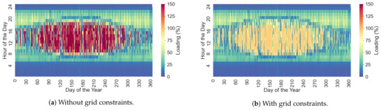
Figure 4.
Main feeder loading with and without the consideration of the grid constraints into the optimization.
3.1.2. Voltage Constraint
Similarly, Figure 5a,b depict the voltage behavior on the PV bus before and after the grid constraints generation.
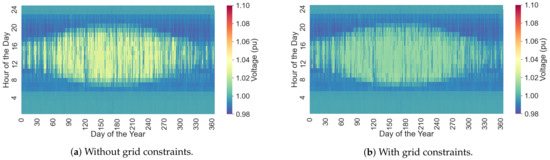
Figure 5.
PV bus voltage at node number 4 with and without the consideration of the grid constraints into the optimization.
Following the same pattern than the over-loading caused by the high in-feed depicted in Figure 4a, voltages above of the nominal voltage occur along with the main feeder over-loading.
Figure 6a,b show the power dispatched by the PV plant before and after the consideration of the voltage and loading constraints of the grid. A noticeable curtailment is needed to maintain the grid quality parameters of loading and voltage within the admissible ranges. The absence of means to store or shift loads during such midday peaks leads to the unavoidable PV curtailment.
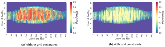
Figure 6.
PV power dispatch optimization with and without the consideration of the grid constraints.
3.2. Heat Pump and Heat Storage
In this section, the proposed methodology is tested by adding some flexibilization technologies such as heat storage and heat pumps.
Even though the installed PV capacity has been decreased to 700 kWp for this scenario, the mismatch between the electric demand and the generation will still create energy flows back to the grid. Such energy flows are big enough to overload the main feeder. As the heat pumps and heat storage are considered in the energy system, the optimizer has the possibility to transfer the energy surplus from the PV system into another energy carrier. Figure 7 shows how the line loading constraint due to the high PV feed-in affects the power dispatch of the heat pumps and PV. The flexibilization of the heat pump activation avoids that the locally generated energy leaves the system. This diminishes the energy injected into the grid, avoiding in this manner the line overloading and diminishing the PV curtailment.
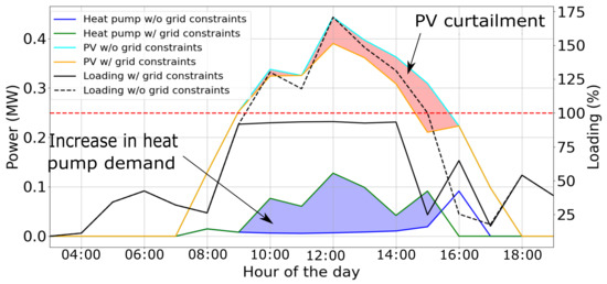
Figure 7.
Flexibilization provided by heat pumps and heat storage. The blue area represents the energy otherwise curtailed without the grid constraints implementation in the dispatch optimization.
Figure 8 shows the variation in energy content in the water storage tank. A noticeable difference is found especially in the months of summer. This is in accordance with the fact that higher values of sun irradiance and less thermal demand are present during such months. Therefore, the heat pumps are continuously being used to tackle PV generation surplus when grid constraint violations occur.
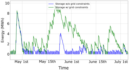
Figure 8.
Change in energy content of the water heat storage.
3.3. Electromobility Scenario
As the fleet of electric cars is added to the energy system, the yearly demand is increased by around 300 MWh. This increment in demand causes line overloads throughout the network. In Figure 9, it can be seen how the main feeder is over-loaded while supplying energy to the EVs during the charging phase. It can be noted that the EV batteries support the grid after they have been connected at 6 pm, which is typically a time of the day with high demand. After the implementation of the constraints into the proposed method, the optimizer re-schedules the EV’s batteries charging and grid feed-in to avoid the overload of the lines.
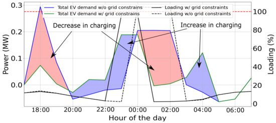
Figure 9.
Cumulative EV charging profile comparison with and without grid constraints.
The proposed method successfully integrates the EV and the distance coverage constraint together with the grid constraints into the dispatch optimization problem of the energy system.
4. Discussion
In Section 3, it was found that the high share of PV at the low voltage level of the electrical system can lead to over-loads at the point of common coupling. This is caused by the residual energy fed into the grid. Neighborhoods with a PV capacity of 10 kWp per household are prompted to lead to grid violations [8]. From the results, it may be inferred that a PV installed capacity of 5 kWp per household can be led to feed-in levels exceeding the nominal voltage in a typical low voltage grid [26]. Nevertheless, over-voltages exceeding of the nominal voltage are very unlikely to occur at this level of penetration. In the case of high share of PV without sector coupling or storage possibility, a curtailment up to ∼60 MWh per year is applied by the method to keep grid limits within acceptable ranges.
The integration of different sector coupling technologies may cause some grid events in the low voltage grids [28,29,30]. However, with a proper control strategy, such technologies can also provide some flexibility to the grid [31,32]. In the scenarios with flexibility options, the method re-schedules the power dispatch from these technologies. Table 2 provides a summary of the influence of the grid constraints in some indicators on each scenario. The summary demonstrates the relevance of the grid constraints in the optimization of an energy system. As it is shown in Table 2, this not only avoids grid limit violations, but it also saves energy from curtailment. From the simulation results, it was found that the methodology here proposed is capable of reducing the energy curtailment up to by adapting to the economic dispatch, the technical grid constraints. Additionally, the self-consumption is increased up to ∼7% per year with the implementation of the method.
Table 2.
Summary of the influence of grid constraints in the optimization parameters. Values are shown in MWh/year.
Therefore, the most economically and technically feasible dispatch of the energy system is achieved. The contribution of the oemof-Solph–PowerFactory toolchain results evident when flexible loads are present in the system. In this regard, the optimization decreases the overall energy that would be otherwise curtailed. Table 3 establishes a comparison between the proposed method and some of the most relevant researches found in the literature.
Table 3.
Comparison with relevant works found in the literature.
Due to the flexibility of energy systems provided by oemof-Solph, the proposed method surpasses the approaches found in the literature in terms of the complexity of the energy system itself. Whereas Martinez et al. [33] consider gas, heat, and power, this study additionally considers, the electromobility sector and the influence on the system by batteries and heat storage. On the other hand, this research only considers the influence of the electric power grid. In some other studies, the grid constraints are considered, but neglecting either storage or other energy sectors [17,34,35].
5. Summary and Outlook
The proposed method combines a linear optimizer such as oemof-Solph and a power analysis tool such as PowerFactory. This combination allows the optimization of an energy system with multiple energy carriers while considering the actual grid limits for sector coupling technologies integration. Such grid limits have an impact on the performance of the energy system:
- For scenarios with PV capacity above 5 kWp per household, the voltage and line loading constraints are violated, therefore affecting the optimization results. In the case study, curtailment of ∼60 MWh/year is needed to keep the grid within its limits. This due to the lack of storage or flexibilization options.
- If flexible technologies are present, parameters as curtailment and self consumption are affected by the grid constraints. In the case study, the self-consumption can increase and the curtailment be reduced by as compared with the typical optimization without grid constraints. The method successfully integrated the additional load from the heat pumps and EV without grid violations.
- In comparison to other approaches, the decoupled constraint generation in the optimization problem determines the techno-economical power dispatch for all the different energy sectors and storage technologies.
To adapt the method to large-scale grids, different open source tools might provide a faster interface and interaction with oemof-Solph compared to the PowerFactory API. Most of these tools are written in python or julia [36]. Another novel approach would be to consider a data-driven constraint generation. This might be especially relevant for online applications or analysis in the transmission system. Due to its high accuracy and run-time, this topic is yet to be exploited [37]. Furthermore, the influence of the heat network is a feature that could be added to this approach in future research.
Author Contributions
Conceptualization, A.R., P.K. and F.S.; investigation, A.R.; writing—original draft, A.R.; supervision, P.K.; writing—review and editing, A.R., P.K., F.S. and K.v.M. All authors have read and agreed to the published version of the manuscript.
Funding
This research received no external funding.
Institutional Review Board Statement
Not applicable.
Informed Consent Statement
Not applicable.
Data Availability Statement
Not applicable.
Conflicts of Interest
The authors declare no conflict of interest.
References
- United Nations Framework Convention on Climate Change (UNFCCC). The Paris Agreement. 2015. Available online: https://unfccc.int/process-and-meetings/the-paris-agreement/the-paris-agreement (accessed on 19 May 2021).
- Agora Energiewende. Energiewende: What do the new laws mean. In Ten Questions and Answers about EEG; Agora Energiewende: Berlin, Germany, 2017; Available online: https://www.agora-energiewende.de/en/publications/energiewende-what-do-the-new-laws-mean/ (accessed on 25 December 2021).
- Bundesministerium für Umwelt, Naturschutz und nukleare Sicherheit. Climate Action in Figures-Facts, Trends and Incentives for German Climate Policy; Federal Ministry for the Environment, Nature Conservation and Nuclear Safety (BMU): Berlin, Germany, 2018. [Google Scholar]
- David, A.; Mathiesen, B.V.; Averfalk, H.; Werner, S.; Lund, H. Heat roadmap Europe: Large-scale electric heat pumps in district heating systems. Energies 2017, 10, 578. [Google Scholar] [CrossRef]
- Sensfuß, F.; Deac, G.; Bernath, C. Vorabanalyse Langfristige Rolle und Modernisierung der Kraft-Wärme-Kopplung; Kurzpapier. Hg. v. Bundesministerium für Wirtschaft und Energie BMWI: Berlin, Germany, 2017. [Google Scholar]
- Jochem, P.; Babrowski, S.; Fichtner, W. Assessing CO2 emissions of electric vehicles in Germany in 2030. Transp. Res. Part A Policy Pract. 2015, 78, 68–83. [Google Scholar] [CrossRef]
- Jain, P.; Jain, T. Assessment of electric vehicle charging load and its impact on electricity market price. In Proceedings of the 2014 International Conference on Connected Vehicles and Expo (ICCVE), Vienna, Austria, 3–7 November 2014; pp. 74–79. [Google Scholar] [CrossRef]
- Arnold, M.; Friede, W.; Myrzik, J. Investigations in low voltage distribution grids with a high penetration of distributed generation and heat pumps. In Proceedings of the 2013 48th International Universities’ Power Engineering Conference (UPEC), Dublin, Ireland, 2–5 September 2013; pp. 1–6. [Google Scholar] [CrossRef]
- Bayer, B.; Matschoss, P.; Thomas, H.; Marian, A. The German experience with integrating photovoltaic systems into the low-voltage grids. Renew. Energy 2018, 119, 129–141. [Google Scholar] [CrossRef]
- Energetisches Nachbarschaftsquartier Fliegerhorst Oldenburg. Available online: https://www.enaq-fliegerhorst.de/ (accessed on 28 April 2021).
- Fortenbacher, P.; Ulbig, A.; Koch, S.; Andersson, G. Grid-constrained optimal predictive power dispatch in large multi-level power systems with renewable energy sources, and storage devices. In Proceedings of the IEEE PES Innovative Smart Grid Technologies, Europe, Istanbul, Turkey, 12–15 October 2014; pp. 1–6. [Google Scholar] [CrossRef]
- Zargar, B.; Monti, A.; Ponci, F.; Martí, J.R. Linear Iterative Power Flow Approach Based on the Current Injection Model of Load and Generator. IEEE Access 2020, 9, 11543–11562. [Google Scholar] [CrossRef]
- Handschin, E.; Kuhn, S.; Rehtanz, C.; Schultz, R.; Waniek, D. Optimaler Kraftwerkseinsatz in Netzengpasssituationen. Innovative Modellierung und Optimierung von Energiesystemen; LIT: Berlin, Germany, 2009; pp. 39–68. ISBN 978-3-8258-1359-8. [Google Scholar]
- Liu, Y.; Zhang, N.; Wang, Y.; Yang, J.; Kang, C. Data-driven power flow linearization: A regression approach. IEEE Trans. Smart Grid 2018, 10, 2569–2580. [Google Scholar] [CrossRef]
- De Novoa, M.; Martinez, L. Optimal Solar PV, Battery Storage, and Smart-Inverter Allocation in Zero-Net-Energy Microgrids Considering the Existing Power System Infrastructure. Ph.D. Thesis, UC Irvine, Irvine, CA, USA, 2020. [Google Scholar]
- Jiang, M.; Guo, Q.; Sun, H.; Ge, H. Decoupled piecewise linear power flow and its application to under voltage load shedding. CSEE J. Power Energy Syst. 2020, 7, 976–985. [Google Scholar]
- Nolden, C.; Schönfelder, M.; Eßer-Frey, A.; Bertsch, V.; Fichtner, W. Network constraints in techno-economic energy system models: Towards more accurate modeling of power flows in long-term energy system models. Energy Syst. 2013, 4, 267–287. [Google Scholar] [CrossRef][Green Version]
- Lohmeier, D.; Cronbach, D.; Drauz, S.R.; Braun, M.; Kneiske, T.M. Pandapipes: An Open-Source Piping Grid Calculation Package for Multi-Energy Grid Simulations. Sustainability 2020, 12, 9899. [Google Scholar] [CrossRef]
- Geidl, M.; Andersson, G. Optimal power flow of multiple energy carriers. IEEE Trans. Power Syst. 2007, 22, 145–155. [Google Scholar] [CrossRef]
- Levron, Y.; Guerrero, J.M.; Beck, Y. Optimal power flow in microgrids with energy storage. IEEE Trans. Power Syst. 2013, 28, 3226–3234. [Google Scholar] [CrossRef]
- Acha, S.; Green, T.C.; Shah, N. Techno-economical tradeoffs from embedded technologies with storage capabilities on electric and gas distribution networks. In Proceedings of the IEEE PES General Meeting, Minneapolis, MN, USA, 25–29 July 2010; pp. 1–8. [Google Scholar] [CrossRef]
- Qadrdan, M.; Ameli, H.; Strbac, G.; Jenkins, N. Efficacy of options to address balancing challenges: Integrated gas and electricity perspectives. Appl. Energy 2017, 190, 181–190. [Google Scholar] [CrossRef]
- Hilpert, S.; Kaldemeyer, C.; Krien, U.; Günther, S.; Wingenbach, C.; Plessmann, G. The Open Energy Modelling Framework (oemof)-A new approach to facilitate open science in energy system modelling. Energy Strategy Rev. 2018, 22, 16–25. [Google Scholar] [CrossRef]
- Gonzalez-Longatt, F.; Torres, J.L.R. Advanced Smart Grid Functionalities Based on Powerfactory; Springer: Berlin/Heidelberg, Germany, 2018. [Google Scholar] [CrossRef]
- Schmeling, L.; Schönfeldt, P.; Klement, P.; Wehkamp, S.; Hanke, B.; Agert, C. Development of a decision-making framework for distributed energy systems in a German district. Energies 2020, 13, 552. [Google Scholar] [CrossRef]
- Forschungsstelle für Energiewirtschaft e.V. (FfE) CC BY 4.0. Basisnetztopologien MONA 2030. Available online: https://www.ffe.de/themen-und-methoden/speicher-und-netze/752-ffe-stellt-rechenfaehige-basisnetztopologien-aus-projekt-mona-2030-zur-verfuegung (accessed on 28 April 2021).
- Ben-Ameur, W.; Neto, J. A constraint generation algorithm for large scale linear programs using multiple-points separation. Math. Program. 2006, 107, 517–537. [Google Scholar] [CrossRef]
- Clement-Nyns, K.; Haesen, E.; Driesen, J. The impact of charging plug-in hybrid electric vehicles on a residential distribution grid. IEEE Trans. Power Syst. 2009, 25, 371–380. [Google Scholar] [CrossRef]
- Passey, R.; Spooner, T.; MacGill, I.; Watt, M.; Syngellakis, K. The potential impacts of grid-connected distributed generation and how to address them: A review of technical and non-technical factors. Energy Policy 2011, 39, 6280–6290. [Google Scholar] [CrossRef]
- Mies, J.J.; Helmus, J.R.; Van den Hoed, R. Estimating the charging profile of individual charge sessions of Electric Vehicles in the Netherlands. World Electr. Veh. J. 2018, 9, 17. [Google Scholar] [CrossRef]
- Hilpert, S. Effects of Decentral Heat Pump Operation on Electricity Storage Requirements in Germany. Energies 2020, 13, 2878. [Google Scholar] [CrossRef]
- Rubio, A.; Behrends, H.; Geißendörfer, S.; Maydell, K.v.; Agert, C. Determination of the required power response of inverters to provide fast frequency support in power systems with low synchronous inertia. Energies 2020, 13, 816. [Google Scholar] [CrossRef]
- Ceseña, E.A.M.; Loukarakis, E.; Good, N.; Mancarella, P. Integrated Electricity–Heat–Gas Systems: Techno–Economic Modeling, Optimization, and Application to Multienergy Districts. Proc. IEEE 2020, 108, 1392–1410. [Google Scholar] [CrossRef]
- Huang, Z.; Fang, B.; Deng, J. Multi-objective optimization strategy for distribution network considering V2G-enabled electric vehicles in building integrated energy system. Prot. Control Mod. Power Syst. 2020, 5, 1–8. [Google Scholar] [CrossRef]
- Clegg, S.; Mancarella, P. Integrated electrical and gas network flexibility assessment in low-carbon multi-energy systems. IEEE Trans. Sustain. Energy 2015, 7, 718–731. [Google Scholar] [CrossRef]
- Auer, S.; Liße, J.; Mandha, S.R.; Horn, C. Power-Flow-Constrained Asset Optimization for Off-Grid Power Systems Using Selected Open-Source Frameworks. In Proceedings of the 4th International Hybrid Power Systems Workshop, Crete, Greece, 22–23 May 2019. [Google Scholar]
- Pineda, S.; Morales, J.M.; Jiménez-Cordero, A. Data-driven screening of network constraints for unit commitment. IEEE Trans. Power Syst. 2020, 35, 3695–3705. [Google Scholar] [CrossRef]


Publisher’s Note: MDPI stays neutral with regard to jurisdictional claims in published maps and institutional affiliations. |
© 2021 by the authors. Licensee MDPI, Basel, Switzerland. This article is an open access article distributed under the terms and conditions of the Creative Commons Attribution (CC BY) license (https://creativecommons.org/licenses/by/4.0/).