1. Introduction
According to Directive 2010/31 of the European Union (EU) [
1], which was established to address the problem of the inefficient use of energy, by 2020 Europe was required to reduce its energy consumption by 20%, and 20% of the total energy consumed should come from renewable energy. Furthermore, the ultimate goal of the energy saving policies in Europe [
2] is to limit by 50% its energy consumption and reduce by at least 80% its greenhouse gas emissions by the year 2050 (compared to 1990 levels).
In recent years, a significant number of scientific research attempting to deal with the current poor energetic performance of buildings is being published. Actually, the building sector is the largest contributor to energy consumption worldwide [
3]. In the European Union in particular, the building industry is responsible for approximately 40% of the total energy consumed [
4].
Among the most mentioned high-impact solutions to the exposed urgent issue is the retrofitting of existing building stock because, while new buildings can be designed and constructed with high-energy performance, a low-energy performance level characterizes most existing buildings. Therefore, construction retrofitting offers significant opportunities for reducing global energy consumption and hence may help to fulfil the European objectives by 2050.
Keeping in mind that the previously mentioned objectives are set for the benefit of us all, the optimization of energy efficiency should be a priority. Furthermore, it is proved that proper energy efficiency measures may also have a positive impact on the indoor environment by improving comfort and maintaining satisfactory services [
5].
In the above-presented context, AP2BEER (Affordable and Adaptable Public Buildings through Energy Efficient Retrofitting) is a project within the 7th Framework Programme of the European Union. Non-residential buildings, especially service buildings, consume 40% more energy than residential ones. Due to this fact, through interventions in tertiary buildings, a greater impact can be achieved [
6]. The A2PBEER project developed a cost-effective energy efficient retrofitting methodology for public buildings with different uses located in different climatic zones in Europe. To achieve thorough research, three public buildings with different uses and located in different climatic areas were selected to participate in the project. The main goal of A2PBEER consisted of monitoring these buildings, then retrofitting them and finally, each building was monitored again to evaluate the energy savings, which should be near 50%. The chosen pilot buildings were the Rectorate of the University of the Basque Country (Spain), the Technology and Maritime Museum at Malmö (Sweden) and Aflivadem Vocational School at Ankara (Turkey). According to the classification of Urge-Vorsatz [
7], the first one is an office building in the Oceanic climatic zone, the second one is a culture centre in the Continental climatic zone and the third one is an educational building in the Mediterranean climatic zone.
The literature of several research works proves that, by appropriate retrofitting, the energy consumption of a building can decrease; however, retrofits usually do not work as well as expected. In many studies, significant differences between the predicted and the operational energy performance, better known as the building energy performance gap, have been found [
8]. Understanding the pre-retrofitting energetic behaviour of the building is a key starting point for the retrofitting. Thus, one of the tasks to be executed in the AP2BEER project included the calibration of the building energy model, defined in the literature [
9] as the process of developing a building energy simulation (BES) by changing parameters and inputs in order to predict as closely as realizable the energy use of the building and the performance of its components and systems. It can be concluded that a calibrated model reduces the energy performance gap between the real energy performance of a certain building and its corresponding energy simulation model, where the mean bias error (MBE) between these results should be lower than 5% on a monthly basis or 10% on an hourly basis [
10].
The building model is considered calibrated when the discrepancy between measurements and predictions does not exceed a given threshold [
11]. This is precisely the goal of this paper: the calibration of a simulation model by using monitoring data information, quantifying the possible differences and justifying them.
This paper is located within “Building Stock” (an example of a non-residential building with heating and appliances) and “Uncertainty” (comparison between monitoring data and white box-based model simulation results) according to the domain of interest proposed by Manfren et al. [
12] for building energy performance studies. For this goal, measurement and verification techniques are applied for the calibration of a simulation model in the operation phase of the building while it is in use [
13].
The energy performance gap tends to be bigger in buildings that are already in operation because there are more uncertainties involving the input data due to parameters related to the occupancy [
14]. These parameters are hard to predict, and it depends strongly on each specific case [
15]. This is why a suitably calibrated model is not easy to reach; for this purpose, the acquisition of verifiable data, the choice of adequate methodology and the use of appropriate tools become very important [
16].
2. Monitoring vs. Simulation
In order to faithfully predict the energy performance of a building, energy models have become a valuable tool [
17]. In response, the interest in BES, which tries to emulate reality and improve the traditional manual methods that have been used to optimize the energy performance of buildings, has increased. In the early years, BES was used in the beginning stages of construction design, but Clarke et al. [
18] emphasize that they can be used at any stage in order to face questions arising during any phase of the life of buildings. In fact, recently, building simulation in the post-construction and in-use stages has significantly risen.
When talking about BES calibration of an in-use building, it should be emphasized the importance of knowing how the building really works. In order to acquire that knowledge, the monitoring of the building is crucial; nevertheless, there is a generalized lack of measured data, which conducts to severely limiting results in most calibration studies [
19]. Measuring can be from basic to detailed: many works use monthly data or utility bills to compare them with the BES [
20], other studies use daily or hourly data taken from short monitoring periods [
21], and others only consider the final energy consumption [
22]. However, lately, the trend is to measure data in more detail, for instance, on an hourly basis for longer periods. Furthermore, in some studies energy consumption was measured separately depending on the end use [
23]. This way, errors due to lack of data are minimized.
It must be emphasized that neither BES nor monitoring are fully reliable. Monitoring devices always have a range of accuracy and simulations are based on the input data, which involve many uncertainties: scenario uncertainties such as building usage/occupancy schedules and building physical or operational uncertainties, modelling assumptions and ignored phenomena. Thus, the calculations made by the program to emulate the performance of the building can differ from the real performance.
Although there is a great interest in the calibration of BES models, there is no agreed or regulated guideline yet on this issue [
16]. Nevertheless, there are many research works describing different methods, some of them validating or questioning them [
24] or even suggesting improvements for further BES calibration works [
23]. In reference [
25] are exposed very usual calibration methodologies, which may be combined in a BES calibration for better results. Some processes rely exclusively on the author’s criteria, and others need specific technical knowledge [
26]. This text aims at providing an exhaustive description of how a BES calibration can be performed using an evidence-based methodology. The proposed procedure is similar to others, where a sequence of data input in calibration is followed [
7,
23]. The proposed methodology is time consuming but simple to apply. The obtained calibrated model will make it easy to further simulate different retrofitting actions and compare the possible energy savings against the actual performance.
There is plenty of research work about retrofitting and calibration methods, but in most cases, papers do not go deep into how the comparison between simulation data and measured data is performed or which steps have been followed during the calibration; normally, only the final result is revealed. The exposed work intends to be an example for further easy-to-perform and accurate BES calibration. To illustrate this process, the BES of the Rectorate of the University of the Basque Country (before its retrofitting) is going to be calibrated, employing the data obtained from monitoring undertaken in the year 2015 while the building was in use.
3. Methodology
As defined in [
25], evidence-based model calibrations are based on adjusting input data and model parameters but only with realistic values according to monitored or audited data. To know the actual energy performance of the building and thus, to know how to determine the building energy model are elementary steps, often overlooked, towards a properly retrofitted building. In this section, a BES calibration procedure is defined step by step; similar calibration procedures have been found in the literature [
7,
23]. However, in order to facilitate further work, two measures have been adopted. On the one hand, calibration methodology has been simplified without adversely affecting its results. On the other hand, the process has been minutely described, from the way in which information has been manipulated to the obtained results, taking into account the conclusions drawn through all the reflections that have emerged in the process of calibration. The methodology differs from others because the calibration is performed at different period scales (weekly, monthly, summer, winter) and analyses not only consumption parameters but also indoor temperature.
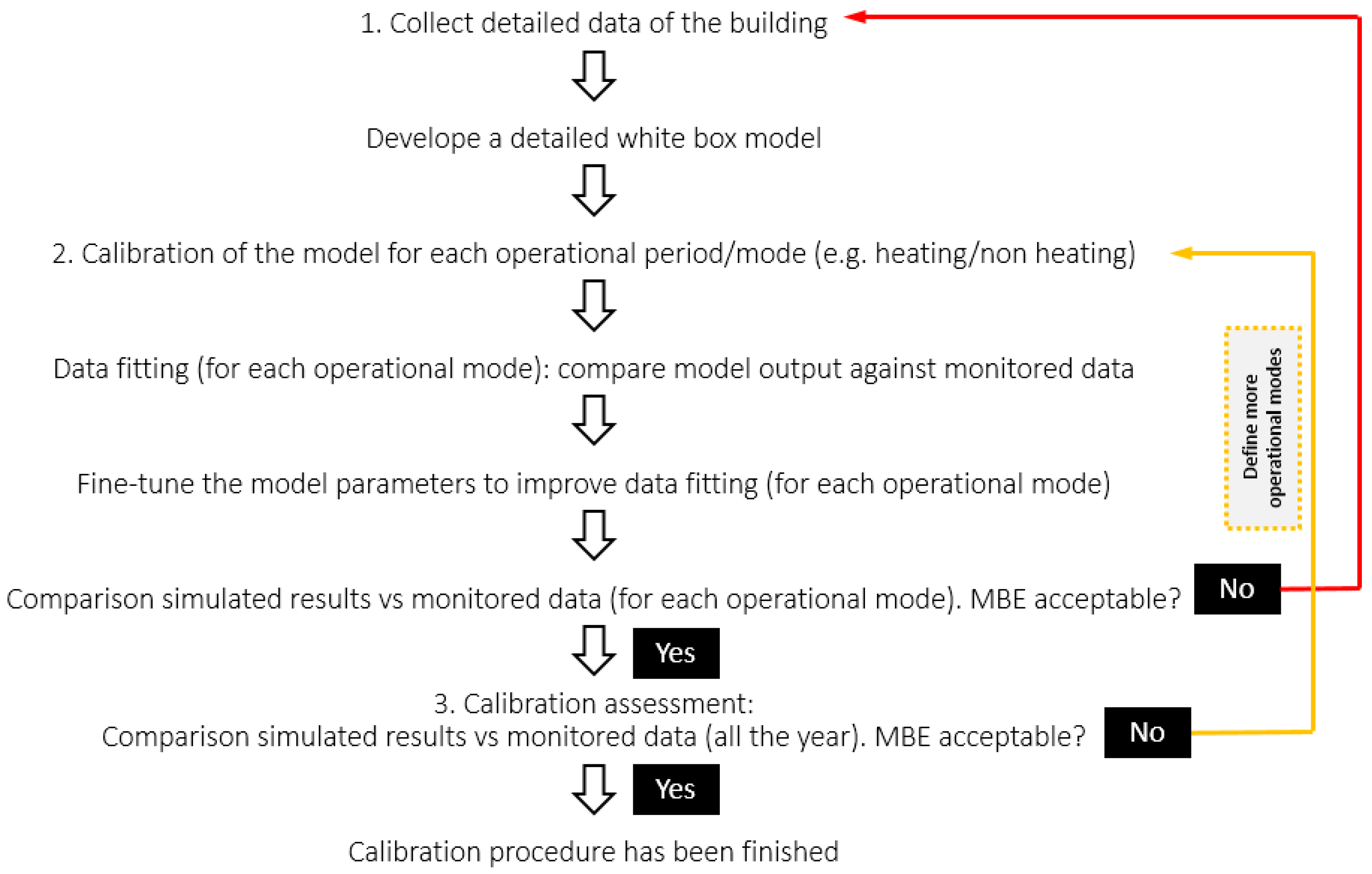
The following stepwise procedure to calibrate the building model has been followed for a robust approach, and in
Figure 1 the procedure can be seen as a flowchart:
- 1.
Understanding the building and its operation (collect reliable information of the building and its surroundings).
- •
Conduct monitoring to know the operation of the building and verify the quality of the obtained data.
- •
Establish a hierarchy for data sources regarding reliability.
- •
Extract information from the monitoring data.
- •
Define operational periods of the building (e.g., heating or not heating periods) and sub-operational periods (e.g., weekday or weekend).
- •
Define operational schedules for the different periods.
- 2.
Calibration of the model
- •
Define zone types of the building model according to its operation and use.
- •
Run a simulation using collected known verifiable data (e.g., using monitored weather data) for each operational period.
- •
Compare the results of each operational period with the monitored data.
- •
If disagreements are found, fine-tune the results and adjust model parameters.
- •
Run the model for a year.
- •
Compare the results with the monitored data.
- 3.
Calibration assessment
- •
If the approach is not acceptable, go back to “Understanding the building and its operation”.
Above-mentioned steps are described in detail below (
Figure 1).
3.1. Understanding the Building
3.1.1. Monitoring
There is a wide range of research focused on the monitoring of buildings to know their real energy performance and their comfort level. It must be stressed that monitoring has to attend to the necessities of each building and its purposes; that is why suitable monitoring for one building can be a bad option for another.
A monitoring campaign has been carried out in the West Block (WB) of the Rectorate building since May 2014. The measurement system follows the standards set by CONCERTO [
27]. Both indoor and outdoor parameters have been measured. Depending on the characteristics of each floor, three or four temperature, relative humidity, CO
2 concentration (T-RH-CO
2) sensors that measure on a minute basis have been installed at strategic places. If no discrepancies are found between sensors on the same floor, the average values are used to calibrate the model (
Figure 2). If discrepancies are found between sensors on the same floor, this must be taken into account in the definition of the thermal zones of the BES model.
In order to synthesize data processing and simplify the comparison with simulation results, measures collected every minute are averaged in hourly intervals. The monitoring system is actually oversized for the purpose of this study. A. Erkoreka [
28] defines the devices installed in the Rectorate Building and their accuracy. As explained in the
Section 4, temperature (°C), relative humidity (%), air quality (CO
2 ppm.) and brightness level (lux) are measured. Heating and lighting energy consumptions are also measured for each floor. The meteorological station is located on the roof of the building.
3.1.2. Data Source Hierarchy
It is worth highlighting that each building is different and that the information available can vary considerably; consequently, information sources should be classified in order of trustworthiness in each case. The proposed sequence for the current study does not use arbitrary data or data derived from mathematics or statistics; all data employed to complete the BES calibration are extracted in order of their reliability from:
Monitoring.
Walk through audits.
Building drawings.
Building project book.
Interviews and surveys.
3.1.3. Data Extraction through Monitoring
Once the monitoring has been realized for the established period and the hierarchy has been defined, it is time to pre-process information from the monitoring data, such as occupancy schedules, use of lighting and heating performance.
The more reliable information is obtained, the more input data and model parameters will be available and the higher the accuracy of the calibration will be. With the objective of minimizing the differences that may exist between the simulation outputs and measured data, the one-year monitored data have been organized monthly regarding: comfort, weather, occupancy, heating and lighting profiles. For a more illustrative analysis, monitoring data have been plotted. This organization process also serves to verify if data sets are complete. In this case, monitoring has failed several times during the year (blackouts), meteorological data have been obtained from other sources, concretely from a meteorological station located 15 km from the building, but energy consumption and comfort data are unknown. This factor is considered when comparing annual and operational season data, pro-rating the results by means of results in similar type days.
3.1.4. Operational Periods
Usually, buildings do not work in the same way throughout the year; there can be heating periods, cooling periods, non-heating and non-cooling periods and occupied and non-occupied periods. Furthermore, usually those operational periods consist of smaller intervals, which are repeated successively, such as weeks where weekdays and the weekend should be differentiated.
Once the data set organizational phase is finished, the different operational periods of the building during the year have been established. Then, a typical sub-operational period has been chosen for each season defined in the previous step. In this case, the year has been divided in two seasons: winter and summer periods. Winter period, from September to June, is the heating (June and the period from September to early November has no heating) and constant occupation period. In the summer period, July and August, the heating system is always off, and occupation can vary a lot from one week to another due to summer holidays. The results of the monitoring demonstrate that the continuously repeated basic use scale is the week. For weekly analysis, one typical week of each season was selected, the second week of February and July 2015.
3.1.5. Operational Schedules
Operational schedules are extracted from monitoring data, and different audits and surveys were carried out. Occupation, heating, lighting and ventilation schedules are defined in detail in
Section 4.6. These have been defined for each season on a weekly basis.
3.2. Calibration of the Model
3.2.1. Zone Types
The thermal zones of a building can be defined according to many criteria. There is a large body of research where only orientation criteria are used, while others are more detailed and take into account space function, adjacency of the exterior, available measured data and conditioning method. In the presented calibration, orientation, use and conditioning characteristics have been considered.
3.2.2. Tool Choice
In practice, it has become common to complete the building energy model using building simulation software to quantify expected energy savings from retrofits, usually on a yearly basis. In this research, the energy performance of the building studied has been simulated for a whole year using a detailed simulation tool that uses the EnergyPlus simulation engine and Design Builder V4.7 (DB), which uses the heat balance-based solution of radiant and convective effects, in combination with heat and mass transfer models for air movements between zones, among others (
Figure 3).
This tool can run the BES, providing detailed hour-by-hour energy analysis of buildings, among other things. Moreover, Design Builder was chosen as the BES tool because it provides an easy way to change both input monitored data (such as monitored weather data) and model parameters (such as envelope thermal properties) during the calibration process.
3.2.3. Weather Data
The building to be calibrated is located in Leioa (near Bilbao). The average temperature fluctuation throughout a day is 7.5 °C, the average temperature throughout the day being 10.6 °C in the heating period and 18.6 °C in the non-heating period. This is because Leioa has a mild climate under the influence of the thermal inertia of the sea due to its proximity to the coast.
The software chosen to perform the BES uses EPW (EnergyPlus weather data) statistical meteorological data. In order to minimize uncertainties between simulation statistical weather data and real weather data (
Figure 4), outdoor conditions were measured and simulation weather data have been replaced by monitored data. For that purpose, monitoring data have been converted into an appropriate weather file.
Figure 4 shows the discrepancies between monitoring data and the simulation EPW file before being changed. Weather data are considered some of the most important uncertainties during a calibration process [
29]. It can be seen that the monitored year is warmer than the one provided by the simulation program. Specifically, there are 4130 HDG
15 (Heating Degree Days) and 1654 CDG
20 (Cooling Degree Days) of difference throughout the year. The global horizontal radiation is quite similar in both cases, except in April. This means that using the EPW file directly would lead to errors in the calibration process. Thus, one of the first steps during the calibration process was to modify it with measured weather data. On the way, two difficulties were faced:
There are measurement gaps for some periods of the year due to technical problems. The following data are missing in weather measurements (blackouts): outdoor temperature and global radiation from 20 May at 10:00 to 2 June at 10:00, from 16 July at 8:00 to 26 August at 11:00 and from 6 October at 14:00 to 8 October at 10:00.
In the monitored weather files generated for the BES software, diffuse horizontal radiation and direct normal radiation are required; however, only the global horizontal radiation has been monitored.
Blackouts have been filled by taking the missing information from Euskalmet (Basque Meteorology Agency). To verify the suitability of the Euskalmet data, days on which monitored data were available were randomly selected. Then, the monitoring and Euskalmet data from those days were compared; the results showed minor differences (
Figure 5), so the weather file was completed with the data from the Basque Meteorology Agency’s measurements.
The second difficulty was estimating the diffuse and direct radiation (requested data in the simulation meteorological EPW file) from the measured global horizontal radiation. The calculation is based on [
30], where the bases of the solar energy are explained, on [
31], where diffuse fraction is calculated through statistics and on [
32], which proposes the calculation method for the diffuse solar irradiation concretely in the north Mediterranean belt. Then, in [
32], different existing correlations between the hourly atmospheric transmissivity (
kt) and the hourly diffuse fraction (
kd) are analysed and finally, a new one is proposed.
kt is the ratio of global-to-extraterrestrial irradiation. For calculation purposes,
kd, which depends on the solar altitude, is expressed into three equations calculated by regression (Equation (1)). The value of
kd and thus the diffuse radiation (global irradiation by
kd) is achieved by applying the corresponding equation on the range where
kt is located:
3.2.4. Calibration Procedure
First, a BES for each sub-operational period was run with available reliable data. To maximize the accuracy in the calibration of the BES, monitored data and simulation results are compared both graphically and numerically, facilitating qualitative and quantitative comparisons to find discrepancies. It must be emphasized that, instead of comparing only the final energy consumption, the Heating, Ventilation and Air Conditioning (HVAC) and lighting energy consumption, the indoor temperature of the building is analysed separately, floor by floor. If disagreements are found, they should be resolved by correcting and adjusting model parameters, always using reliable data only.
First, the suitability of sub-operation periods (week period) must be checked. If disagreements are detected, they should be solved by changing model parameters or checking if the sub-period is well chosen.
Finally, the building model was simulated for the whole year. The process for the different time periods of calibration proposed is repeated. To complete the simulation of periods with missing monitored data, the available data are used to estimate the average behaviour of each month.
3.3. Calibration Assessment
Currently, three standards describe when the BES can be considered calibrated: ASHRAE Guideline 14 [
10], Measurement and Verification guidelines (M&V) [
33] and the International Performance Measurement and Verification Protocol (IPMVP) [
34]. All three are based on measured data and statistical indexes, such as the mean bias error (MBE) (Equation (2)). These parameters evaluate how similar the energy consumption of the simulation model is with reality. Nevertheless, as Fabrizio and Moneti stress in [
11], these validations do not guarantee that the input data of the BES model fit with reality.
where
mi is the measured data of a certain variable during the chosen time interval,
si is the simulated data of a certain variable during the chosen time interval and
Np is the number of data points of the interval.
Most articles use the aforementioned criteria to evaluate whether their modelled building is sufficiently calibrated or not.
4. Building Description
This section explains how the above-presented calibration procedure has been applied to an office building of a university campus. Before proceeding to calibrate the model, input parameters and variables need to be defined; the information source hierarchy is defined in
Section 3.1.2.
Built in the 1970s in Leioa, near Bilbao (Spain), the building studied is the Rectorate building of the University of the Basque Country. This office building is a complex made up of three blocks, as can be seen in
Figure 6: the west block (WB), central block (CB) and east block (EB). Although three blocks are connected by corridors and have the same heating system, only the WB was monitored. Furthermore, there are other buildings in the campus with similar construction features; therefore, the retrofitting works could be repeated in those constructions.
The WB consists of a ground floor plus three others, and it is oriented in the north-south direction. The west facade of the WB is external; in contrast, in the east a party wall separates the WB and the central block of the Rectorate building, and for calculation purposes this area shall be considered adiabatic.
Figure 7 shows the floor plans and the uses of the WB of the building, which are represented with different colours. The Rectorate is mainly an office building (brown), but on the ground floor there is a nursery (green). There are also various rooms used as storage rooms (grey), passage areas (pink) and a place where the servers of the UPV/EHU (blue) are located.
Below, a brief description of each floor of the WB:
The ground floor (GF) is the largest. The nursery, located on the west side, is the only heated area on this floor; the rest of the surface belongs mostly to non-conditioned areas, such as storage rooms, accesses to the building and circulation areas.
First floor (F1) has four individual office rooms on the northwest corner, but it is mainly an open space. On this floor, the local server, which has an independent air conditioning system that allows for dissipation of the heat generated by the equipment, maintaining its temperature at 22 °C almost constantly throughout the year, is located in the southeast corner.
On the second floor (F2), two different areas can easily be distinguished, the north and south oriented areas. Both contain many small office rooms, so the occupation in this floor is lower than on the floor below, F1. The biggest differences between the two zones are the orientation and that the areas that face to the north have no false ceiling; therefore, there is a greater volume of air to be conditioned.
Third floor (F3) is the smallest. This is the space reserved for the staff responsible for informatics on the campus. In this mostly open space, excepting two individual office rooms and a meeting room, there are a lot of internal loads, mainly due to the elevated use of computers. This floor has a distinguishing characteristic, the skylight, so solar gains will be higher than on the other floors.
4.1. Geometry
The four-storey building has a maximum height of 18 m. Although the floor plans are irregular, they can be considered rectangular-shaped, and they measure 30 × 22 m (only the WB). The structure is simple, consisting of concrete pillars and grid concrete slabs.
Data sources used to fill the
Table 1 parameters are taken from the original project memory and drawings of the project; to ensure that the information is correct, some in situ measures were also taken. No significant differences were found among them.
In the BES model, thermal zones of the building must be defined (which have an impact on the results [
23]). The WB has been divided into different zones, taking into account two factors: the use of the rooms and their orientation. Each small floor plan view of
Figure 7 represents the thermal zones introduced in the simulation program to complete the building model.
4.2. Thermal Envelope
The analysed building has been partially renovated several times throughout its life. Thus, the building envelope is complex with several local interventions to be considered. The facade is mainly composed of two prefabricated reinforced concrete panels with a non-ventilated air chamber between them (
Table 1). On the south facade, which has no surrounding buildings, there are reinforced concrete sunscreens that shade glazing in summer and provide solar gain in winter. The only insulated element is the roof of the third floor.
The original windows have wooden carpentry and simple glass, but there are windows with aluminium frames and double-glazing on the first floor and in some places of the north facade.
Table 2 is a summary of the characteristics of the building windows (g, solar factor and U, thermal transmittance).
Average estimated infiltration rates have also been introduced in the calibrated simulation: 0.2 ACH (air changes per hour). The infiltration value was calculated with the methodology used in [
35] analysing the CO
2 decay curves.
4.3. HVAC
The HVAC system of the building is simple since there is no hot water demand, no mechanical ventilation supply or any refrigeration system. While no centralized cooling system is provided, some rooms have autonomous air conditioning equipment, but this effect is neglected in the calculations. Besides, the building is naturally ventilated through operable windows.
Natural ventilation is difficult to estimate because it depends on the behaviour of the occupants. Usually, the windows are opened when users feel hot. Certain circumstances are established to define the use of ventilation: windows are opened while the building is occupied when inside the building the temperature exceeds 26 °C, regardless of the outside temperature. There is an exception; in the nursery, windows are always opened while occupied, as observed in all visits to the building.
The existing heating system is centralized (district heating), and it serves all campus buildings. The facility is composed of seven modulating boilers running on natural gas, one of which feeds the Rectorate building heating system. The rooms are heated by two groups of radiators: one for the north orientation and the other one for the south orientation.
After analysing the monitored data in the heating period months, the working set point temperature has been adjusted to 23.5 °C. As in some floors the peak temperature of the simulation compared to the monitored data is not reached, the set point was increased by 1 °C or 2 °C.
4.4. Lighting
Predominantly, fluorescents provide the internal lighting, and most of them are constantly turned on while the building is occupied, both in summer (season with more natural light hours) and in winter. That is why no significant differences were found between the consumption of these seasons.
4.5. Thermal Loads
The aim of this section is to define the internal thermal gains (
Table 3); for that purpose, walk-through audits (A), surveys and measurements were carried out in order to obtain information about:
Number of lighting gadgets, their power and operation schedules. It is worth noting that in the first audit broken bulbs were found, and that was an additional reason to carefully analyse monitoring data (M).
Plug appliances, such as desktop computers, were also counted. Information about the quantity, the power and the operation was extracted from the audits.
It is not easy work to obtain detailed occupancy data from monitoring. Occupancy surveys and audits during different days were carried out. The estimation of the occupation is an average value of the information acquired; rare days were discarded.
In the case of the thermal load definition, the monitored data, instead of being the main source of information, were helpful for checking the rightness of the site survey data due to difficulties found with extracting information such as occupation:
The maximum lighting power of each floor measured in January and March was contrasted with the total power obtained from the walk-through audits. It has been considered that, at least once a month (remember that measures were taken hourly), all lighting was on simultaneously. Most values were similar, so they were considered correct. However, on F1 a considerable difference was found; while audits estimated a total lighting power of 8305 W, the measurements revealed a lower power of 7513 W. The differences have been attached to non-replaced broken lights; in the second audit, this issue was verified.
CO2 measurements were used to find out if each floor of the building was occupied or not, but no relation between instantaneous occupancy values and CO2 measurements was conducted. Therefore, occupation values were exclusively taken from walk-through audits. The average observed values have been used. In the software, the occupation (pers/m2) schedules must be defined. Occupant thermal gains depend on their activity level; these values are quantified by the simulation software.
At this stage, the metabolic conditions of users must be defined; the same value has been considered for all of them. In this case, due to the building type and usage, light office work activity was chosen with a heat generation of 127 W/person.
4.6. Schedules
In general, schedules are different depending on the season of the year (heating season or cooling season) and the day of the week (weekend or weekdays). Schedules can also vary depending on the floor of the building. However, lighting consumption is almost the same throughout the year on each floor.
From the monitored data, different schedules have been deduced depending on several factors; in the next lines, they are studied by type of consumption:
LIGHTING: As shown in
Figure 8, there is light consumption between 7:00 h and 20:00 h to 21:00 h on all the floors excepting F2, in which consumption ends at 18:00 h. Early in the day, the light consumption is somewhat lower, probably because at that hour staff continue to commute to work; therefore, not all lights are switched on. There is a drop in the consumption early in the afternoon on the GF, matching the naptime in the children’s nursery. On F1 and F2, in the afternoon, the decrease in energy consumption is staggered.
Lighting consumption is very similar throughout the year. Even if in the summer season power peaks are slightly lower, schedules in the BES were considered equal on each floor during the whole year. However, there is an exception: in August, the nursery is closed, so there is no lighting consumption in that month. On weekends, the lights are off according to the monitored measurements. Otherwise, consumption is fairly constant throughout the day, as can be observed in
Figure 9.
HEATING: There are two heating periods. In the summer season, from June to September, the heating system is switched off, while the rest of the year it operates on a set schedule. The heating turns on at 6:00 h and turns off at 19:00 h. The heating system regulates the power supplied to maintain the temperature set point. A slight relationship between the heating consumption and outside temperature was detected from the monitoring data. In winter, during the warm hours of the hot days (such as 2 February, Monday at midday) heat consumption falls. This is because the heating system works as a function of the outdoor temperature. When the outdoor temperature is higher than 18 °C, the heating system switches off. The heating system works under the same schedule all over the building, and it is noteworthy that early in the morning, when the heating is turned on, there is a peak in the consumption that it is quickly stabilized. Then, the consumption is more or less constant until it is switched off. The peak is due to the extra energy consumption required to reach the set point temperature early in the morning. Special days have been detected in the operation of the building. For example, even if the heating programming is off on weekends, sometimes the heating turns on to avoid over-cooling of the building. This is why a second set point of the heating programming is fixed at 18 °C.
OCCUPATION: Occupation schedules (
Figure 9) are the result of analysing the collected schedules from the surveys and the CO
2 measurements in the GF, F1, F2 and F3. From September to June, occupation is regular on each floor during weekdays, and the building is empty on weekends and holidays. During summer (July and August), the occupation varies considerably depending on the day; in general, the occupation is lower and there are less working hours. No occupancy is found in the nursery during this period.
TEMPERATURE: Temperatures in F1, F2 and F3 are similar; however, on the GF, although the maximum temperatures are equal to those of the rest of the floors, at night they are much lower. The difference is greater than 5 degrees. This issue is explained in
Section 5.2.
5. Results
Monitoring data of the Rectorate are available from May 2014; however, this study analyses a whole year (from 1 January 2015 to 31 December 2015). Monitoring was interrupted several times during 2015.
Section 3.2.3 explains how the missing data were completed regarding the weather data. It also explains the procedure followed for those days where there was no monitored data of the consumed energy nor of the indoor comfort data. This fact shall be taken into account when comparing the simulation and monitored data of different operational seasons and the whole year.
First, a typical week has to be chosen for the winter and summer model calibrations. Once the weekly calibration is finished, the results for the whole year will be analysed.
5.1. Week Selection for the Analysis
In order to know if the weekly operational pattern in a floor is repeated over time, on all floors a four-week analysis was conducted floor by floor. In
Figure 10, the monitoring data (lighting energy consumption, CO
2 concentration and temperature) of the second floor has been plotted as an example to compare heating and non-heating periods. The results of this analysis show whether the week chosen is suitable to calibrate each operational season. For heating period analysis, 4 weeks of February were chosen, and for non-heating season the last 2 weeks of June and the first two of July were selected in order to analyse the building energy performance with a high occupancy rate. It must be taken into account that occupation should be lower in July and August due to vacations.
CO2 patterns give an idea of occupation and ventilation habits in the building. The CO2 graphics show that in summer natural ventilation is higher compared to the winter season. This is because natural ventilation is directly related with the outside temperature conditions; the higher the temperature is, the higher the natural ventilation due to window openings. There is also a slight difference between profiles of June and July due to occupation. When the CO2 concentration is analysed, it should be noted that it is never lower than 400 ppm, because this is the outdoor ambient CO2 concentration. Illumination distribution throughout the year is the same, with less intensity in the summer period.
In June–July, the temperature is closely related with the exterior weather conditions, while in February temperature profiles are more regular because the heating system is working according to the energy consumption of
Figure 11.
Figure 10 shows that indoor temperature graphics are qualitatively and quantitatively very similar in the winter season, despite the exterior meteorological conditions being slightly different depending on the week. This is because the indoor temperature in winter is directly dependent of the heating system, as it has been mentioned above. Consequently, due to the differences in the outdoor temperature, heating power must also be different depending on the week (
Figure 11).
For the outdoor temperature analysis, 15 °C based hourly heating degree-days in February is considered: in week 1, 1879.7 HDG15; in week 2, 1001.7 HDG15; in week 3, 1057.2 HDG15; in week 4, 909.6 HDG15. The coldest and warmest weeks are week 1 and week 4, respectively. That is the reason why quantitative differences are found in the heating energy consumption profiles.
It is notable that heating consumption is higher during the coldest week (week 1). In the morning, there is always a need to warm up the building, which is why the consumption is similar during all weeks. However, higher differences have been found in the afternoons because different power is required to maintain the indoor temperature, depending on the outer temperature conditions.
As a conclusion, no differences were found in the thermal behaviour of the building for the analysed weeks, except the dependency of heating (in winter) and the indoor temperature (in summer) with the outdoor temperature. On the other hand, different values and schedules for occupation, lighting power and natural ventilation were taken into account in the BES model, in order to consider their influence over the heating and non-heating periods. For the weekly model calibration, the second week of July and February were selected for the non-heating and heating periods, respectively. However, the selection of these weeks should not influence the calibration process, as long as there are no outliers such as holidays.
5.2. Weekly Model Calibration
With all the collected information, two BES models were run, one for each chosen typical week: the second week of February 2015 (winter) and the second week of July 2015 (summer).
First, the summer simulation was carried out to check if the indoor temperature and lighting levels were acceptable. In the first step, the indoor temperature is studied floor-by-floor (
Figure 12) and MBE results are also analysed.
According to indoor temperature, the MBE values on all floors were below 5%, except for the GF (11.7%). After an audit, the reason for the mismatch was found: between the GF and the F1, there is a ventilated air chamber of 1.5 m in contact with the outdoor environment. Whereas the floor of the F1 is insulated, the roof of the GF is not. In summer, the maximum and minimum temperatures differ from the rest of the floors. In winter, however, only the minimum temperatures are different. This is because the heating system, which works under a set temperature, is properly working.
Hereafter, GF results are excluded from the analysis. The indoor temperature and heating consumption of the GF are highly influenced by the roof’s ventilated air chamber behaviour, which cannot be simulated properly in DB. This chamber makes the indoor temperature of the GF very dependent of the outdoor temperature and also on solar radiation, since big window areas are present in the west façade.
For the summer, the building averaged the lighting consumption per square metre, and the indoor temperature comparison between the simulated and monitored results can be graphically evaluated in
Figure 13.
Once similar temperatures are obtained for simulation and monitoring in a typical summer week, winter week illumination and temperature are checked (building averaged). In this case, heating power was also studied (
Figure 14).
In winter, the indoor temperature is higher in the monitored data compared to the simulated model results. The temperature difference is bigger when the heating system is not working, especially at night. To minimize this difference, the inner thermal mass (furniture, partitions) of the building was implemented in the model. Still, the indoor temperatures at night are higher in reality compared to the simulated data. As can be seen in
Figure 14, the simulation program does not consider all the heat stored within the hot water confined in the heating system, which is slowly given to the building, even during the night. Meanwhile, in the simulation, heating consumption falls sharply at 19:00 h, and monitoring data show a negative exponential fall. That is the reason why the largest discrepancies are found in the heating consumption.
5.3. Year Model Calibration
Once the model calibration has been developed for summer and winter typical weeks, the comparison of the results will be shown for the whole year. For a better comparison and agreement between monitored and simulated results, two aspects have to be considered:
Not all monitored data from the analysed year (2015) are available during different periods due to technical problems. Monitoring in the summer months has not worked most of the time. August and July have 1487 h and only 366 h have been measured. Therefore, any calibration assessment would not be real, even only considering data from the monitored dates. In the winter months, monitoring interruptions were occasional; the season has 7273 h and 6941 h have been measured. In the BES model, holidays and vacations are not taken into account. According to the monitored data in these days, there is no energy consumption, except if the indoor temperature is below 18 °C (a few times during the year). In January, April and December there are several holidays.
In order to make a proper comparison, results have been prorated with the purpose of completing the missing monitored data and to take into account holidays. An extrapolation has been made to avoid discrepancies due to the lack of monitored data and holidays. Only lighting and heating consumption are showed because they are the most important consumptions in office buildings (
Figure 15).
BES results show a good agreement with reality (measured data). Lighting and heating simulation consumptions are in line with the monitored data.
5.4. Calibration Assessment
At this point, the suitability of the calibrated model has to be quantified numerically by means of MBE. BES models are considered to be calibrated if their MBE value is lower than 5% in the monthly criteria or 10% in the hourly criteria, according to ASHRAE Guideline 14 [
10].
It must be highlighted that for this analysis the GF results have been discarded because in the simulation the roof’s ventilated air chamber could not be taken into account with the same thermal effect as in the real building.
Despite the great variability in parameters to be defined in BES models, the results from
Table 4 show a good agreement between the simulation results and monitored data. The annual lighting and heating MBE results do not reach the ASHRAE criteria by less than 1%.
6. Discussion
After all the previous analysis (both graphical and numerical), the BES model can be considered calibrated. This calibrated model will allow for the prediction of reliable estimations of energy savings for different retrofitting scenarios of the building.
Lighting has been the easiest task to calibrate because the lighting power is one of the variables that has been measured. Furthermore, during occupation hours, most of the spaces are occupied, both in summer and in winter periods; therefore, all the lighting is usually switched on. Only a lowered consumption is shown in summer, which is related to the low occupancy of the building and therefore to empty rooms. Notice that the building has fixed shading elements on the south façade to prevent solar radiation gains in summer. These elements cause insufficient natural light to work.
Heating and temperature calibrations are more complex since many parameters affect them. Some are difficult to measure, and others are unknown: in the weekly comparisons, it was seen that in the monitored data the drop in heating consumption is a negative exponential, while in the simulation it falls sharply as the system is switched off. Besides, in the simulation the heating consumption is slightly bigger than in the monitoring.
The first difference is because the real system (monitoring) and simulated system do not work equally. Monitoring considers the real heating system operation, which has a recirculation pump that moves the hot fluid while there is still hot water in the pipes (although the boilers are off). However, for the simulation program, as soon as the heating system (boilers) is turned off there is no heating power supply to the building. The fact is that the simulation does not consider that the residual heat in the tubes causes a higher and a faster decrease of temperature inside the building when heating is turned off (at night). In fact, analysing the weekend data, although at the beginning the simulated temperatures are lower than the monitored values, there is a point at the end of the weekend where minimum temperatures have the same value for the monitored and simulated data. This is because after the residual heat has been dissipated, temperatures tend to equalize gradually. Just for this reason, as temperatures overnight are lower, the simulated heating system has to work more in the early morning to achieve the temperature set point, making the consumption greater.
Finally, according to some authors, MBE is not the most suitable parameter due to the cancellation effect between positive and negative biases. However, the main purpose of the calibration of simulation models (as in this case) consists of achieving similar annual average results between the simulation and the real consumption, in order to accurately estimate the real energy savings for different retrofitting scenarios.
7. Conclusions
An energy monitoring system has been designed and deployed to be implemented in a BES model calibration of the Rectorate Building of the University of the Basque Country. The definition of monitoring standards could be a step forward to normalize the BES model calibration methodology because it could reduce uncertainties due to the intervention of the author in the monitoring definition process. In this study, a minimum set of variables to be measured are defined to energetically characterize an in-use office building.
In the literature, when a building energy model is calibrated, the procedure employed is not normally revealed in detail. Most of the studies are only limited to the results and basic guidelines definition. This text presents the calibration of a building from the information acquisition phase to validation step by step.
The available monitoring data have been used in the whole model calibration procedure. They have been used to firstly better understand the in-use operational schedule of the building. They have also been used to understand the thermal behaviour of different thermal zones of the building. Then, some of the monitoring variables have been used as inputs to the model, and others have been used as outputs to check the quality of the model calibration. This whole procedure of data analysis has been developed in detail in this article.
In essence, the methodology is simple; it consists of calibrating the building for the operational seasons established and checking if the calibration is appropriate at different operational scales. If building drawings, construction details and building operational data are available, it has been proven that the calibration is easy to perform. The hardest part is the data handling. The more reliable information is available, the easier it will be to calibrate the BES model. On the other hand, the more uncertainties exist in the available data, the more assumptions must be made when making the calibration process, which is very dependent on author assumptions. It must be highlighted that it has been proven that a short monitoring period is not enough to perform a detailed BES calibration.


 ,
, 


