Abstract
In shipboard DC grids, tightly controlled load converters can impair the system stability, thus provoking the ship blackout. Conversely, load converters regulated by low control bandwidths are capable of inducing a stabilizing action. This compensation is verifiable if the loads are few. On the contrary, the balancing of control dynamics is hardly evaluated if the bus feeds multiple (i.e., hundreds or more) DC controlled loads. In this paper, the weighted bandwidth method (WBM) is presented to assess the small-signal stability of a complex shipboard power system by aggregating the multiple converters into two sets of controlled loads. Once the validity of the aggregation is proven, a stability study is performed on the two-loads system. As the last system is more inclined to instability than the initial multiple-loads system, the verification of the two-loads stability criterion guarantees that the shipboard DC grid also remains stable. Finally, emulations on HIL verify the proposed stability assessment thus providing the first unique verification of WBM.
1. Introduction
Developments in power electronics promote the exploitation of DC technology both in on-land distribution systems [1,2] and in shipboard power grids [3,4,5]. By focusing on the marine context, the DC paradigm offers several advantages, both in low (LV) and medium voltage (MV) applications [6,7,8]. Regarding the MVDC case, the IEEE Std. 1709 has described points of strength but also the open challenges [9]. Among the pros, a pervasive power conversion to DC provides a reduction in power system volume and an enhanced modularity in ship design [10,11]. Conversely, DC applications can exhibit an unstable behavior, investigated since the 90s [12,13] until the present day [14]. When the penetration of power electronics is high, as in DC grids, the dynamics interactions between controlled converters and filters can deteriorate the system’s stable operation. Indeed, if an LC input filter feeds a tightly controlled converter modeled as constant power load (CPL), small voltage sags on the DC bus can trigger voltage oscillations, and therefore instability. In this regard, refs [15,16] are important contributions for identifying the CPL instability issue and a possible control strategy to compensate for the destabilizing effect. From these milestones, several approaches have been proposed as effective in solving the CPL destabilizing effect. First, a discussion about the stability issue on shipboard DC grid is in [17]. Then, ref [18] discussed the CPL effect on terrestrial DC microgrids with an emphasis on stabilizing techniques. Other important contributions to DC stability are in [19,20], whereas [21] proposes the concept of a smart resistor to maintain the proper stability margin with minimized filter capacitors. Important work the one proposed in [22], where the loop-cancellation technique is tested with experimental results. Also the authors of the present paper have had a good experience with the linearization via state feedback. Indeed [23,24] are examples where this complex strategy is capable of ensuring system stability even in risky conditions (e.g., generating system disconnection, wrong parameters estimation). Albeit the ideal CPL model is not the worst case from a control standpoint [25], the DC stability assessment is usually performed by adopting the nonlinear CPL on the load side, as it prefigures a well-recognized destabilizing case. Another case in which the CPL hypothesis is conveniently assumed is in [26], where the researchers put the focus on the method for designing a fault-tolerant stabilizing system. CPL is also adopted for marine applications [27,28], while [29] considers a limitation in CPL bandwidth. Other ideas to overcome the ideal CPL are in [30,31], where reduced-order models are defined. Although these models can take into account how the control bandwidths influence the stability of two DC-DC cascaded converters, the methodology will be different when modeling large DC systems. In fact, if the embarked controlled loads are hundreds, as in naval electric ships [32], the DC shipboard microgrid becomes indeed very complex [33,34], consequently compromising the analytical stability assessment. This last aspect is also faced in [35] for a DC electric vehicles recharging infrastructure, where small-signal stability is negatively influenced by multiple supply stations with the same power and control bandwidth. Based on these examples, it is important to observe that the complexity in analytically evaluating the stability of a multiconverter DC power system is not related to the adopted stability criteria, but to issues of modeling activities. Indeed, in the last twenty years an important experience about DC stability has been developed. First, a valuable contribution on stability metrics is provided in [36]. Then, a complete treatise about criteria is given in [37], whereas other important works have specifically discussed about the possible methods for the stability assessment. For giving an idea, it is possible to enumerate the passivity-based stability criterion [38], the impedance-based system method [39,40,41] and the eigenvalue-based method [42,43]. Conversely, in authors knowledge, there is a sort of lack in defining a practical methodology to aggregate the stabilizing/destabilizing effect of controlled loads. As this desirable aggregation can simplify the stability analysis of complex DC grids, therefore the paper is interested in proposing this new Weighted Bandwidth Method (WBM). In authors opinion, this methodology can give a first analytical view about stability issues in isolated-radial DC grids with a pervasive presence of DC-DC controlled converters.
In this paper, the WBM is proposed as an original methodology to weigh how a controlled converter (i.e., its bandwidth) impacts on overall system stability. The WBM is therefore a novel technique for analytically assessing the small-signal stability of multiconverter DC power systems in the presence of very dispersed power and control bandwidth ratings. Such a method models a radial shipboard DC microgrid by means of an approximated DC system. The WBM makes it possible to aggregate multiple-controlled loads into two resulting loads, whose control bandwidths are linear combinations of the original ones. The approximated WBM-based model maintains the total power of the initial complex DC power system and results in smaller stability margins. Therefore, the stability assessment of the WBM-based model is expected to be less conservative. In other words, when the WBM-based model is working at the stability margin, the multiple-loads model is certainly stable. If the stability criteria [36,37,38,39,40,41,42,43] are satisfied for the WBM-based model, a stable evolution results when the initial multiple-loads model is perturbed. The stability assessment based on WBM-based model is then validated by means of emulations on high-fidelity Typhoon HIL platform. These tests prove the WBM capability in aggregating the dynamics interactions of a complex DC grid into two resulting controlled loads. If a perturbation does not compromise the stability of the two-loads aggregated system, also the complex DC shipboard power system results stable in the same perturbed condition.
The paper is organized as follows. Section 2 presents the DC power system, while the WBM-based model is described in Section 3 after the aggregation of multiple controlled loads has been defined. The methodology to study the DC stability of a two-load system is presented in Section 4. In Section 5, the HIL emulations on the initial multiconverter DC system verify the validity of WBM stability assessment. Finally, Section 6 reports the conclusions.
2. DC Microgrid Modeling
The DC power system topology is described in Section 2.1, while Section 2.2 shows the assumptions to simplify the system modeling. In Section 2.3, the analytical model is discussed with particular attention on the output impedance and the input admittance.
2.1. Power System Topology
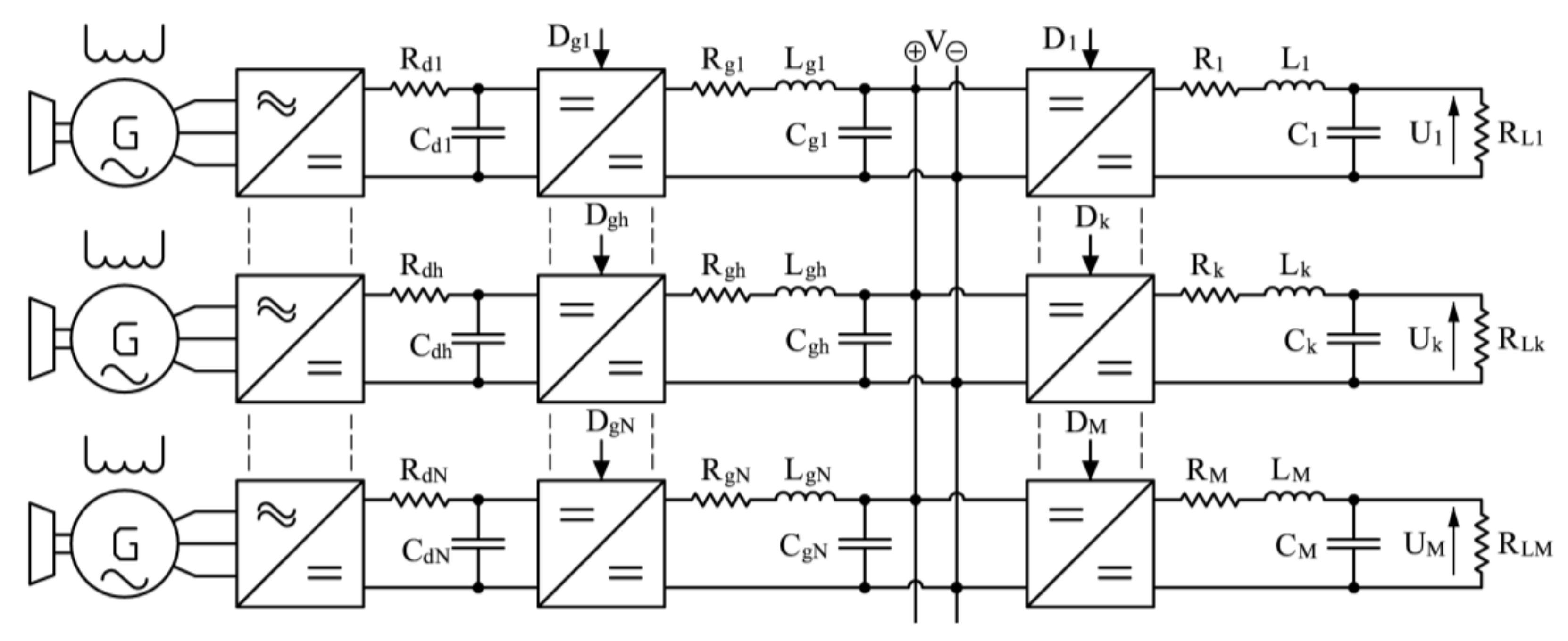
The DC controlled grid is shown in Figure 1. This radial topology has N generating systems (left part) and M load systems on the right of the DC central bus. Each h-generating system (h = 1…N) is composed by the cascade of an AC synchronous machine, diode rectifier and DC-DC interface converter. The AC generator voltage is controlled by an Automatic Voltage Regulator operating on the excitation system, while the duty cycle Dgh is the DC-DC converter’s control signal. Both AC-DC and DC-DC buck converters outputs are filtered, thus a first order arrangement for the diode converter while LC stages are adopted for the interface to the bus. The k-system (k = 1…M) is a filtered DC-DC buck converter feeding the RLk load. The latter is an embarked load (e.g., propulsion, instrumentation, hotel load, low-voltage load), whose voltage is regulated by the DC-DC converter k (i.e., control signal Dk). As specified in [9], a multiconverter DC microgrid like the one depicted in Figure 1 can well represent a future onboard DC system. The authors are therefore interested in studying such a radial example with several interface converters.

Figure 1.
Complex DC Power System (radial topology, N generating systems, M controlled loads).
2.2. Modeling Assumptions and Range of Validity
Numerous control loops are required to manage the DC system in Figure 1. The 2N loops regulate the DC bus voltage (N on AC machines and N on DC-DC converters), while M feedbacks control the voltage on DC loads. The converters’ current controls add extra M loops for the loads and additional N in the generating section. Overall, the DC grid works on the interacting action of B = 3N + 2M control loops. In a complex shipboard DC grid, the B number is therefore in the hundreds, so it follows that the stability assessment is almost unachievable as closed-form expressions. By considering this, three hypotheses simplify the DC model for a particular range of control bandwidths. The consequent stability analysis is also limited to the same range of validity.
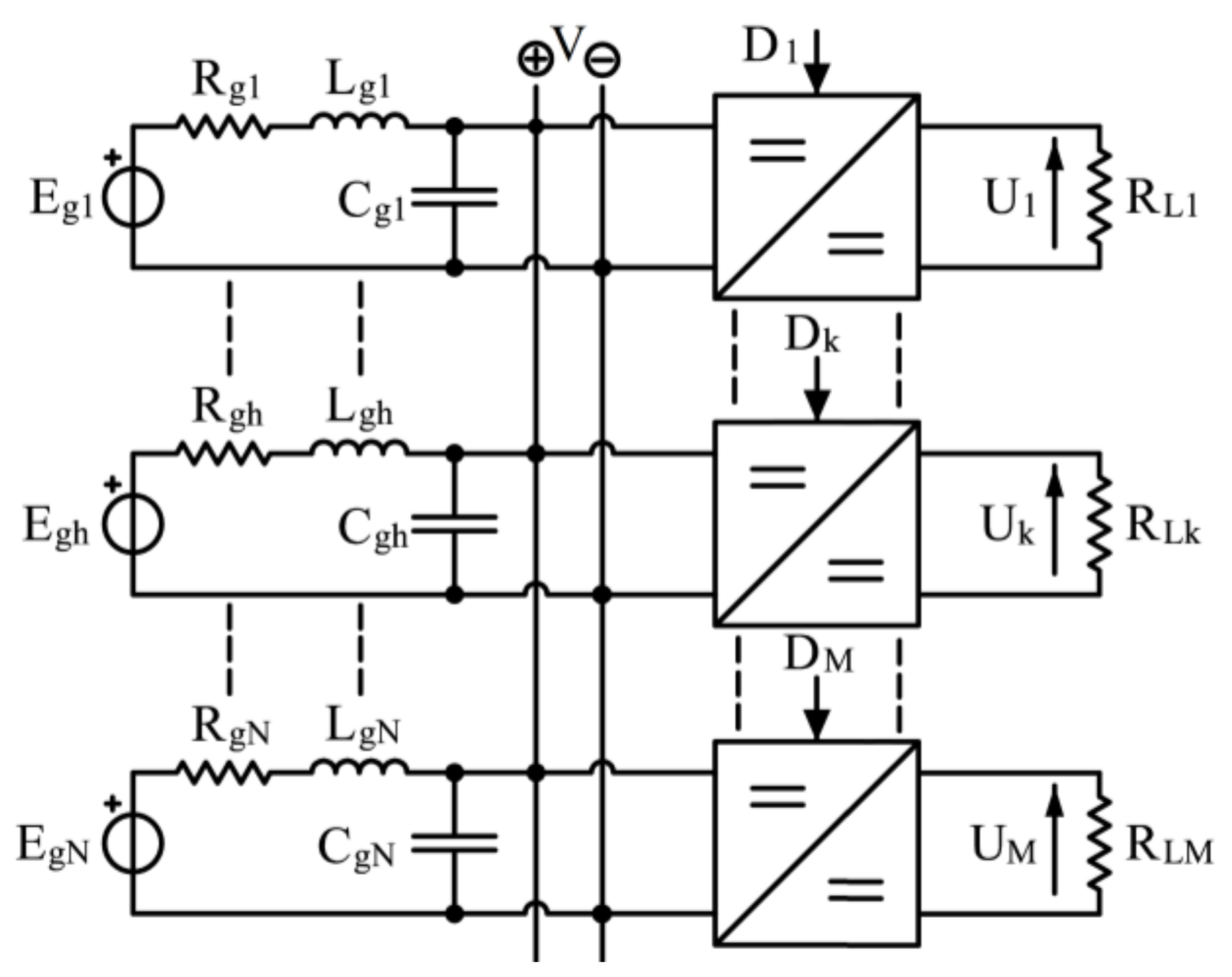
The first hypothesis is on the current loop of each DC-DC converter. As the current control bandwidth is supposed to be ten times larger than the voltage control bandwidth, the inner current loop is negligible as well as its dynamics effect. The second assumption is for each LC filter on DC load. When the Uk voltage is regulated by a first-order dynamics with ωk bandwidth, the k-filter does not affect the bus stability if ωk is sufficiently smaller than the filter’s resonance frequency ωfk. The load filter can be thus neglected as in [30,31]. A final condition is set by comparing voltage control bandwidths of generating/load DC-DC converters. If the ωh bandwidths are ten time smaller than the ωk ones, then the h-converters are assumed to operate in steady state condition. Consequently each h-filter is supplied by a constant voltage Egh (i.e., average value at h-converter output). Apart from the first hypothesis which is quite common in power electronics, the other two are synthesized as ωh << ωk << ωfk, then defining the range of validity. The complex DC microgrid can be simplified as in Figure 2 supposing that the three assumptions are verified.
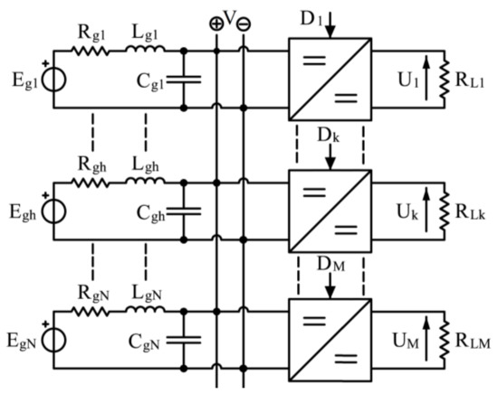
Figure 2.
Microgrid simplification under modeling assumptions.
2.3. Analytical Model
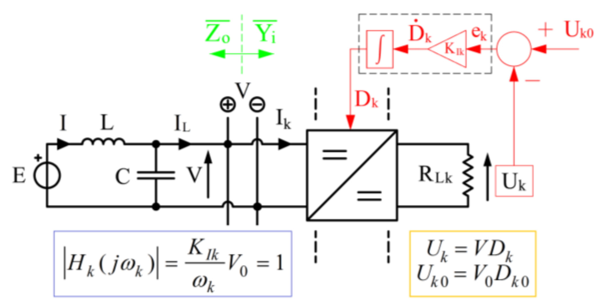
Since the Rgh filter resistors are practically ignored (i.e., small values), the N filters can be aggregated in a Thevenin equivalent circuit as in Figure 3. Now, the E equivalent voltage source feeds the LC parallel-resulting components, while the M voltage-controlled converters are clamped on the capacitor then supplied from the DC bus voltage. Each k-converter is feedback controlled to regulate the Uk voltage on RLk load, thus imposing the Uk0 reference in steady state condition. To simplify the analysis, the fast nonlinear switching dynamics of each converter is disregarded, thus resulting in average value models [9]. As the switching frequency is high, the converter dynamics is indeed negligible because the related pole is placed far beyond the considered field of study in the Gauss plane. Then, the controlled Uk output is given by the product between V average bus voltage and Dk duty signal (yellow box), while the equations with 0 subscript are in steady state. The duty cycle is the output of an integral regulator (dashed box), whose KIk gain imposes a first-order behavior as control target for the Uk output voltage. Once the converter dynamics are neglected, the open-loop transfer function Hk(s) is the cascade of the integral regulator and V0 gain. The KIk value is set for the 0 dB crossing in ωk bandwidth (blue box). Finally, the IL total current is the sum of M input currents Ik. Thanks to above mentioned assumptions, now 2 + M state Equation (1) model the filtered DC microgrid supplying M voltage controlled converters. The first two equations are apparent, the third is defined in Figure 3. Here, Dk first derivative is determined from the red scheme, while Uk, Uk0 and Kik are in yellow/blue box. In the last equation, the M load currents are moved at the converters inputs (i.e., Dk action) to get the total IL. For a small-signal stability study, Equation (1) is linearized in a stable equilibrium point given by 2 + M rated values (V0, I0, Dk0). The model in (2) is then processed by the Laplace transform to find functions V(s) and IL(s), as in (3)–(4). Output impedance Zo(s) and input admittance Yi(s) are in (5), where ω0 = (LC)−0.5 is the equivalent filter’s resonant angular frequency. As in [36,37,38,39,40,41,42], the system stability is evaluated on T(jω) = Zo(jω)·Yi(jω). Thus, Equation (5) is combined in (6) to define the real-imaginary part of T(s), where Gk = Dk02/RLk is the k-conductance and ω the angular frequency.
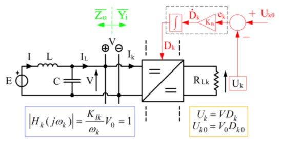
Figure 3.
Controlled DC-DC converter supplied by a filtered DC bus.
3. Weighted Bandwidth Method
Conventionally, the study on product T(jω) is adopted to verify the DC system stability [36,37,38,39,40,41,42]. The same methodology is used for the Figure 1 radial distribution, where the Yi(jω) input admittance (5b) models M controlled converters feeding M loads. As M is hundreds in a ship, the Yi(jω) definition becomes complicated, making the stability evaluation analytically impracticable. The loads aggregation approach adopted here can limit the terms in Yi(jω), enabling a consequent linear modeling. By exploiting this aggregation, the WBM can analytically investigate the stability in complex DC grids, where the several converters can negatively interact while reducing the stability margin. As expressed in the following, the paper novelty is not on the application of well-known stability criteria. Conversely, the novelty is put on the methodology to obtain a simplified model from an initial multiconverter power grid. As the simplified model is representative of the complex one, a stability study on the simplified grid can provide important information about the stability of complex DC microgrid.
3.1. Set Membership
The M loads having ωk bandwidth are gathered in two sets (i.e., S and D), once elected the ωB bandwidth as splitter. The splitter is the bandwidth to put a uniform DC system (i.e., same parameters as study case, except M equal bandwidths,) at the stability boundary (i.e., ℜ[Zo∙Yi] = −1). When the identical ωk are larger than ωB, the uniform controlled system is unstable (i.e., ℜ[Zo∙Yi] < −1). The ωB limit is thus identified by two steps. Firstly, ℑ[Zo∙Yi] is nullified in (7a) to find the critical angular frequency, ω = ωcr = ωB. By putting ωcr in the real part of (7b) while adding up the M conductances as GL, Equation (8) is consequent and ωB the positive solution (9). In the not uniform system, a load belongs to S stabilizing-loads set when its control bandwidth is smaller than ωB. Conversely, the D destabilizing-loads set groups all the controlled loads with ωk > ωB.
3.2. Loads Order and Power Equivalence
To form the S-D sets, the initial M loads are firstly rearranged in increasing order of bandwidth by renaming their subscript (i.e., now ω1 < … < ωB < … < ωM). Similarly, also the subscripts of other parameters are redefined. Then, ωB limit (9) subdivides the loads in the S-D sets, respectively counting MS and MD elements (i.e., M = MS + MD). The S loads have ωk < ωB where k = 1…MS, while the bandwidths of D loads exceed the ωB value (i.e., ωk > ωB, k = MS + 1…M). The WBM is conceived to ensure the power equivalence between the initial M loads and the aggregated S-D loads. Thus, total load power PL and total conductance GL are split as in (10), where GS and GD are the equivalent conductances, while PS and PD the relative powers.
3.3. Linear Combinations of Control Bandwidths
In the definition of S-D sets, the WBM must assure power equivalence and bandwidths aggregation. If the first target is achieved by (10a), the second deserves attention. The bandwidths aggregation law must produce a WBM-based model whose stability margins are lower than the ones of the initial complex DC model. When comparing the multiple-loads model and the WBM-based model, the second one must be more inclined to instability: in other words it reaches the stability boundary when feeding a smaller load. On the other hand, the aggregation law must be basic, thus based on a linear mathematical relationship, in order to simplify the stability assessment during the power system design. By starting from the S set, the Yi(jω) admittance and the YS(jω) aggregated admittance are in (11).
The Yi(jω) in (11a) models the MS loads (i.e., ωk bandwidths, k = 1…MS, ωk < ωB), while the YS(jω) represents a single stabilizing controlled load having a hypothetical ωS control bandwidth. The complexity in (11a) equation is evident when the sum of MS fractions is considered. On the contrary, the aggregated admittance in (11b) has a structure similar to (11a) but a single ωS bandwidth term. The latter is defined in (12a) as a linear combination of the S control bandwidths, weighted by the conductance ratio mk = Gk/GS = Pk/PS. Thus, ωS is a sort of center of gravity, whose definition derives from an analogy to the approximated method (i.e., current-line length products) to calculate the aggregated voltage drop of distributed loads in power systems [44,45]. The same procedure on D loads provides the ωD aggregated control bandwidth in (12b). The linear combinations in (12) and the equivalent conductances in (10b) are the data used to specify the WBM-based model. Once the laws are defined in (12), the validity of the aggregated control bandwidths can be proven as in Section 3.4.
3.4. WBM Less Conservativeness
This Section verifies that the WBM is less conservative [46,47] and its application provides a resulting model with stability margins smaller than the ones of the initial DC complex model. To this aim, the 12 test-model and the related WBM-based model are compared to provide proof. In the 12 model, an LC filtered voltage E feeds two parallel connected DC-DC converters, named 1 and 2. A single controlled converter is shown in Figure 3. The two control bandwidths ω1 and ω2 are stabilizing (i.e., ωk < ωB), while G1 and G2 are the load conductances from the converters inputs. Consequently, each conductance takes into account both the supplied resistive load and the steady state duty cycle on feeding converter (i.e., Gk = Dk02/RLk). By applying the WBM and the small-signal hypothesis (i.e., now the voltage source is ΔE), the 2-loads grid is aggregated into a S single load system, which has the same voltage input ΔE, the equivalent conductance GS (i.e., GS = G1 + G2 = m1GS + m2GS) and the aggregated bandwidth ωS = m1ω1 + m2ω2 (12a). To compare 12 and S models, Equation (2) is rearranged to define the transfer functions from ΔE to ΔV, as in (13), (14). By using (11), the last equations are modified in (15), (16). The W12(s) transfer function (15) is particularized when m1 = 1 and m2 = 0, thus ωS = ω1 (12a). In this case, W12(s) equates (16). Equality appears also in the second limit case, when m1 = 0 and m2 = 1. In order to demonstrate that the WBM was less conservative in the middle condition (m1 = m2 = 0.5), a possible approach identifies the maximum GS after which the two systems are unstable. For the S model, the GSS limit conductance is found in (17) by studying Zo(jω)∙YS(jω) if q = 1. The imaginary part of the last product is nullified when ω = ωcr = ωS. Such a value is thus substituted in the real part to finally find the GSS. An identical procedure is followed in (18) to define the GS12 conductance in the middle condition, where ωcr = (ω1∙ω2)−0.5 is the critical angular frequency for the 12 model. If m1 = m2 = 0.5 and q = 1, the difference ΔG = GS12 − GSS in (19) is always positive, whatever the bandwidths ω1 ≠ ω2. Thus, the WBM’s lesser conservativeness is verified under three conditions (i.e., m1 = 1 and m2 = 0, m1 = 0 and m2 = 0, m1 = m2 = 0.5) for the S stabilizing loads (i.e., q = 1). Similar remarks for the D loads, where initial as well as aggregated bandwidths are above the ωB limit. Indeed, by replaying the same approach when q > 1, the WBM can be again tested also on the D loads set, being GD12 > GDD. As ΔG results positive in the S-D cases, both aggregated controlled loads are definitely more inclined to instability in the three exemplifying positions. To complete the proof, the two studies on ΔG can be extended to the entire m2 range, since the Routh-Hurwitz criterion [30,31] analytically identifies the limit conductances for each m2 value. Once it is verified that the WBM is less conservative with few controlled loads, the same methodology is then directly applicable on numerous loads by updating Equations (10) and (12).
4. DC Stability Analysis
Section 3 has conceived the WBM to gather the controlled loads in two sets. Since aggregated loads are equivalent in power to the initial ones, but more inclined to instability, this Section investigates the DC grid stability by means of the WBM-based model.
4.1. Stability Criterion
The Nyquist criterion is able to assess the stability of the initial DC grid feeding M controlled loads. As in [36], this criterion proves the system stability when the curve Zo(jω)∙Yi(jω) does not clockwise-encircle the point (−1,0) on the Gauss plane. A consequent approach determines the stability behavior by checking if ℜ[Zo∙Yi] > −1 when ℑ[Zo∙Yi] = 0. When the real part is compliant with this condition, the Nyquist criterion is verified then the stability is guaranteed. On the base of this statement, Equation (20) result consequent if adopting (6)-(10)-(12) to define the WBM-based model. The first Equation (20a) is rearranged as in (21) to find the square ωcr, whereas the system stability is ensured when the actual ψ term is less than 1 in (20b).
4.2. Iterative Process for WBM Stability Assessment
By considering Equation (20), the simple iterative process of Figure 4 is developed for two targets. First, the stability behavior of the WBM-based model is evaluated when ωS and ωD are initially defined. Subsequently, the process could be used to properly redefine the two control bandwidths if the initial assessment proved the instability. The first step of the iterative process finds the square ωcr (21), once assigned power system data (green box) and control bandwidths (red/blue boxes). Then, the square ωcr is substituted in (20b) to determine the real coordinate ψ at step 2. This value is compared to the stability target Λ at step 3. When ψ ≤ Λ, the process is stopped as the stability is certainly ensured being Λ ≤ 1 by definition. Conversely, when ψ > Λ the iterative process (dashed lines) can also redesign ωS and ωD to lower the ψ till the Λ value. As the DC stability is impaired by large bandwidth controlled loads [30,31], the iterative process applies a bandwidths reduction to recover the stability requirement. To follow this strategy, the error e is at first determined as ψ−Λ (step 4). Then, both blue and red paths (step 5) can minimize e, then forcing a position near the point (−Λ, 0). By focusing on the blue process, the error is the information to reduce step-by-step the ωS. As this bandwidth gradually decreases at each iterative cycle, the error e similarly moves towards zero. When e is smaller than a threshold (e.g., 10−3), the related ωS is thus able to assure the target Λ. Similar considerations are used for the red path, while lowering the ωD. The basic idea of the iterative process is considered as an advantage, as its application results also simple as a consequence. A complex process to establish the stability performance would be less useful when pursuing the effective implementation in the marine operative context. Moreover, the tuning (i.e., up/down) on ωS and ωD is definitely an effective, although elementary, approach to reaching the stability goal, while preserving the dynamics requirements for as long as possible. Future research activities will be based on this redesign, thus introducing the possibility of smart tuning the control bandwidths.
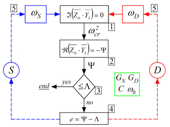
Figure 4.
Stability assessment iterative process implementing the WBM.
5. Validation of WBM Stability Assessment
The WBM aggregates the controlled loads in two sets, whose stabilizing-destabilizing effect is valued by the iterative process. Therefore, this process can provide a first check on stability performance. Then, some studies on poles placement and real-time HIL emulations are able to confirm the process results. When the iterative process is recognized as effective in studying the stability, its application is consequent and well-received.
5.1. Power System Data
A DC system feeding four controlled loads (M = 4) with a radial topology as in Figure 1 and a total power PL = 24 MW is analyzed here. This DC grid is assumed to be supplied by two generating systems (N = 2), already designed in [23,24]. These groups have a total power Pg1 + Pg2 = 15.75 + 10.5 = 26.25 MW. Once we disregard the Rgh as in Section 2.3, the Thevenin equivalent parameters of input filters are L = 1.048 mH and C = 577.26 μF (i.e., ω0 = 1286 rad/s). For the studied case, four RLk loads are fed by DC-DC controlled buck converters. Each load converter is filtered by an LC stage to ensure the power quality [9]. As in [23,24], there are several inputs to size the filters: converter rated power (Pnk), input-output rated voltage (Vn, Unk), rated duty cycle (Dnk), rated output current (Ink) and switching frequency (fsk). Secondly, ΔV% and ΔI% (peak-peak voltage/current ripple) are the filter goals, while ΔP% models the converter losses (percentage). The design as in [23,24] provides Rfk, Lfk and Cfk for each filtered converter, whilst ωfk = (LfkCfk)−1 is the k-filter resonance frequency and RLk is the k load resistance as square Unk subdivided by power Pnk. The power system data are summarized in Table 1.

Table 1.
Parameters for modeling the load section.
5.2. Test Setup
The DC grid has four controlled loads. Depending on the bandwidth, each load can foster stability, or it can provoke unstable behaviors. To evaluate the bandwidths’ effects, three different cases are configured in Table 2. From the bandwidths of Case 1, the ω2 is lowered in Case 2. Then, the bandwidths on load 3–4 are additionally decreased in Case 3. By observing the trend on bandwidths, the system stability improves from Case 1 to Case 3. The WBM stability assessment is able to evaluate this enhancement. A loads modification behaves as a perturbation to check system stability. From the initial condition with four stable loads (i.e., PL = 24 MW), the disconnection of the lowest bandwidth (i.e., stabilizing) converter reduces the total power (i.e., PL = 19 MW) and deteriorates the stability margins. In the following, the last point is discussed.
Table 2.
Control bandwidths configurations.
5.3. Stability Assessment
The ωB splitter groups the loads in the S-D sets for what concerns the control bandwidths. The ωB values in Table 3 confirm that ω2 always behaves as stabilizer since it is smaller than ωB both before and after the perturbation. Similarly, also load 1 helps the stability balance until its disconnection. Conversely, converters 3–4 are always destabilizers as the related bandwidth overtakes the ωB splitter. Once classified the loads before/after the perturbation, the PS and PD total powers in Table 3 are the sum of stabilizing/destabilizing converters powers (Table 1). Such values are used to relativize the single converter power as mk ratio (e.g., m3 = P3/PD = 5/15 = 0.33). From Equations (10)–(12), the ωS and ωD bandwidths are calculated as in Table 4. As the perturbation changes the power ratios of stabilizing loads (i.e., m1 and m2), consequently also the ωS is characterized by two values, before and after the perturbation. Conversely, the ωD is not modified by the load disconnection, as the related power ratios of destabilizing loads (i.e., m3 and m4) are not influenced by the perturbation.
Table 3.
Control bandwidths configurations.
Table 4.
Control bandwidths configurations.
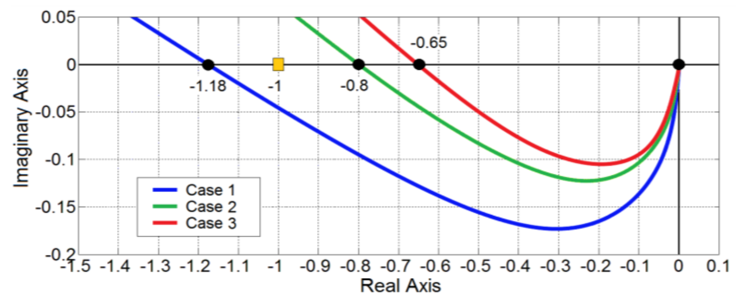
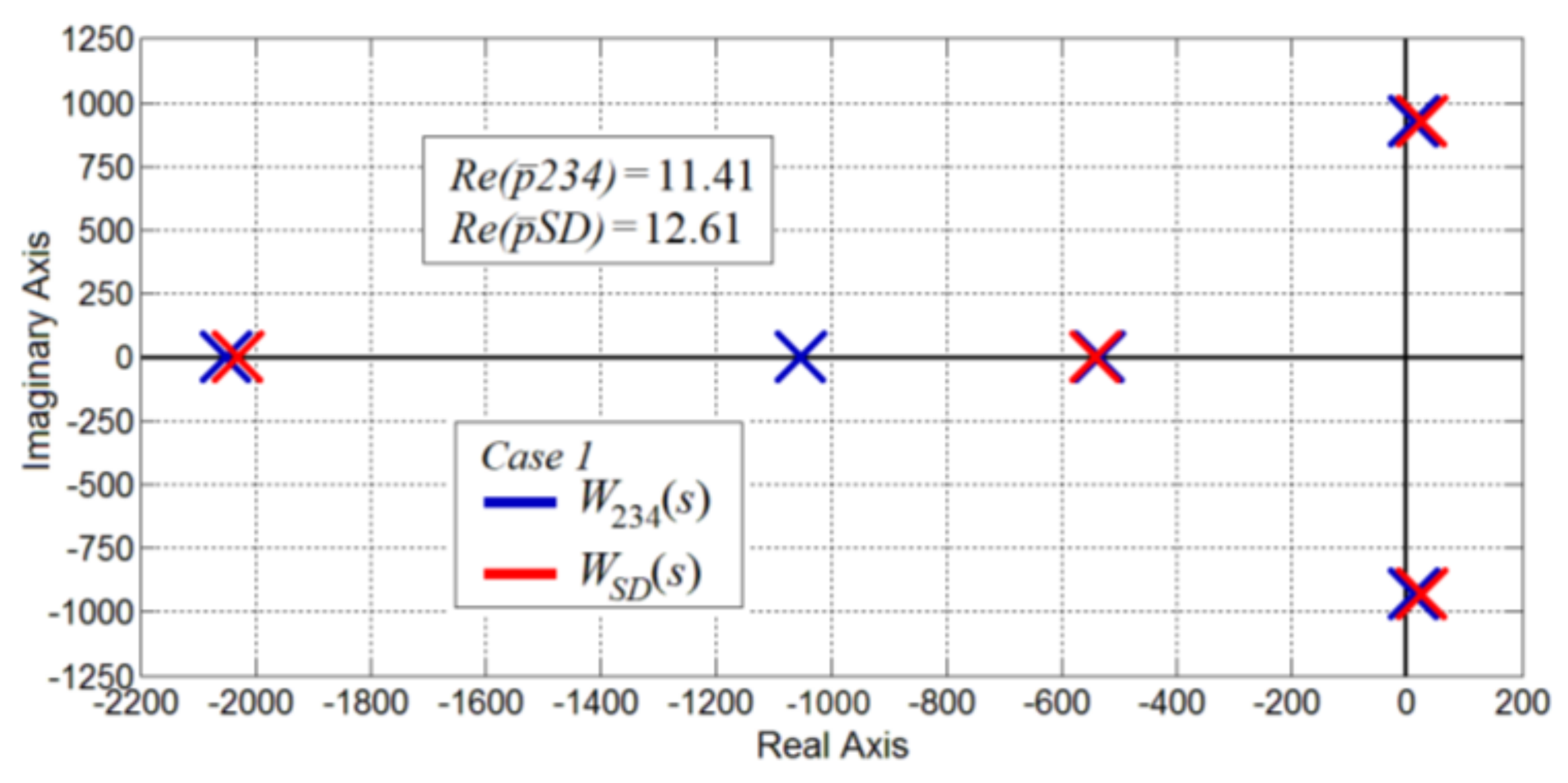
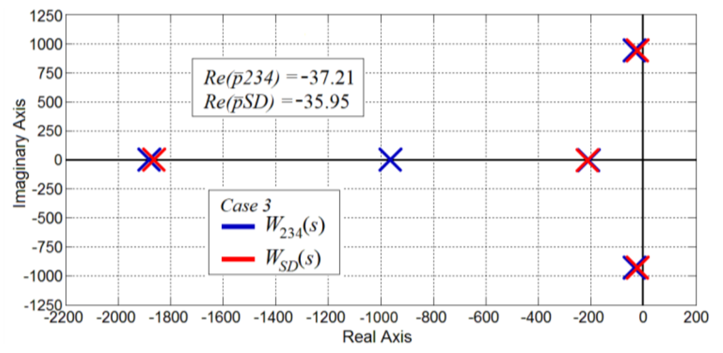
Once the ωS-ωD aggregated bandwidths are defined as in Table 4, the iterative process of Figure 4 is run to establish the stability performance of each case. Particularly, the Nyquist diagram of Figure 5 highlights three intersections. The instability is made evident for the Case 1, where the perturbation is capable of imposing an intersection Ψ = 1.18 > 1. Conversely, the bandwidth reduction on ω2 (i.e., 500–200) in Case 2 is enough to ensure the system stability after perturbation (i.e., Ψ = 0.8 < 1). Finally, Case 3 where the additional reduction on destabilizing bandwidths (i.e., ω3 and ω4) is able to guarantee the best stability result (i.e., Ψ = 0.65 < 1). Being PD more than three times the PS, a tiny reduction (−8.6%) in ωD is sufficient to get the stability target in the last case. Finally, Figure 6 and Figure 7 show the poles of transfer functions W(s) from ΔE to ΔV (15) and (16), when load 1 is OFF in Case 1 and 3. In both cases, the aggregated complex poles SD are always slightly on the right of initial complex poles 234. By comparing their real parts, the relative errors (i.e., 10% in Case 1, 3.4% in Case 3) prove the less conservativeness of WBM stability assessment.

Figure 5.
Nyquist diagram for the control bandwidths design.
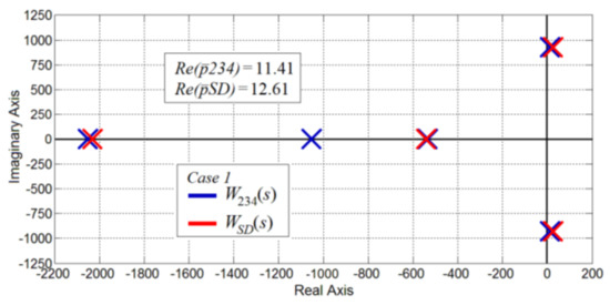
Figure 6.
System poles, transfer function W(s) (Case 1).
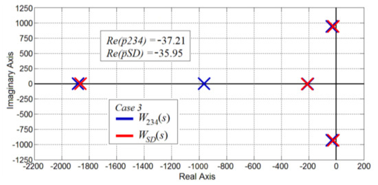
Figure 7.
System poles, transfer function W(s) (Case 3).
5.4. Hardware in the Loop Validation
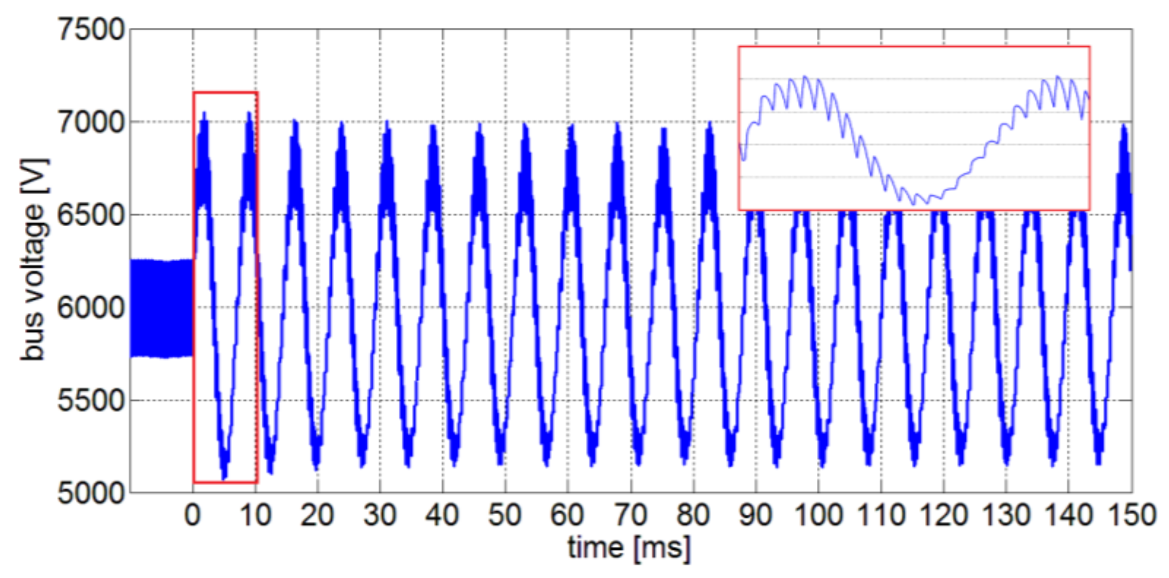
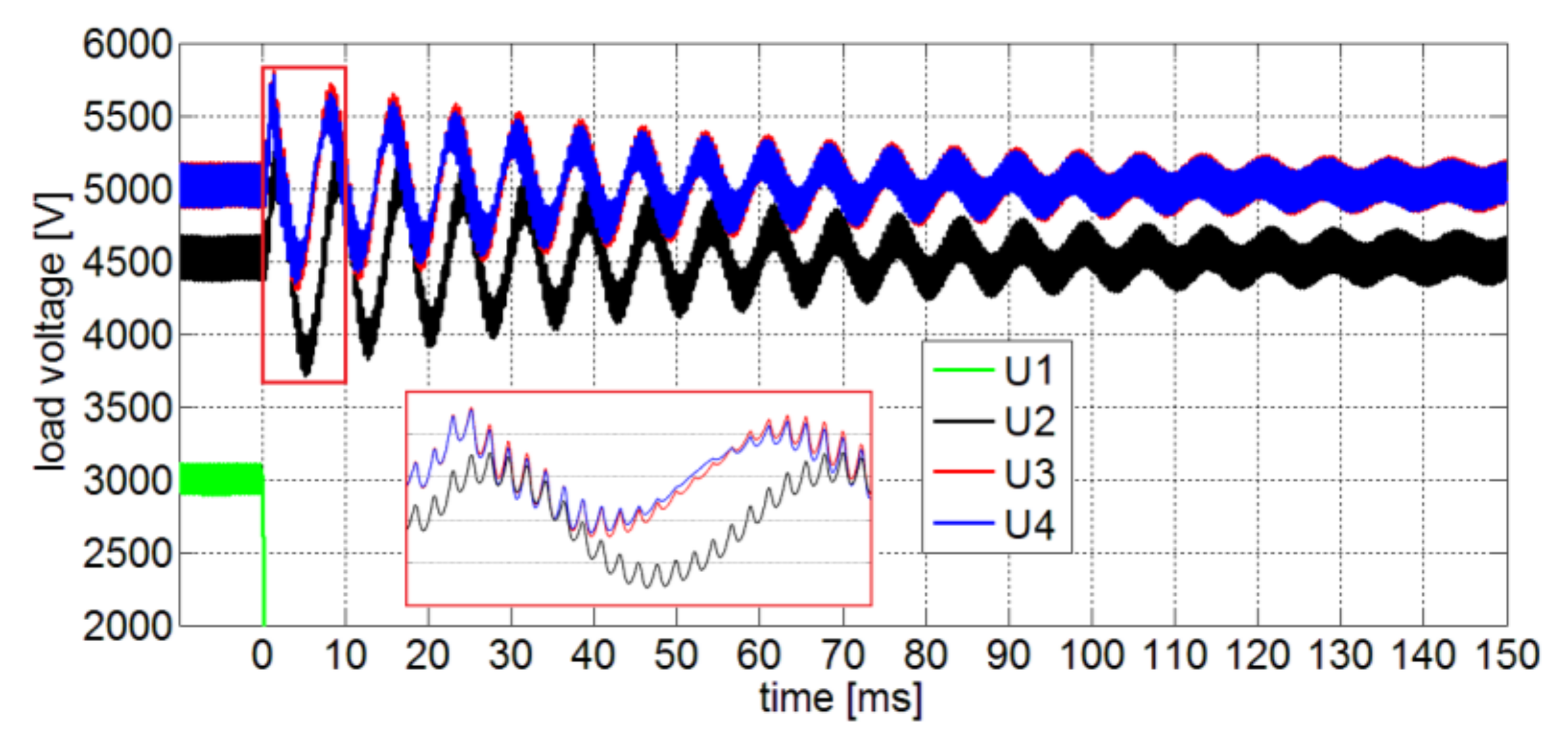
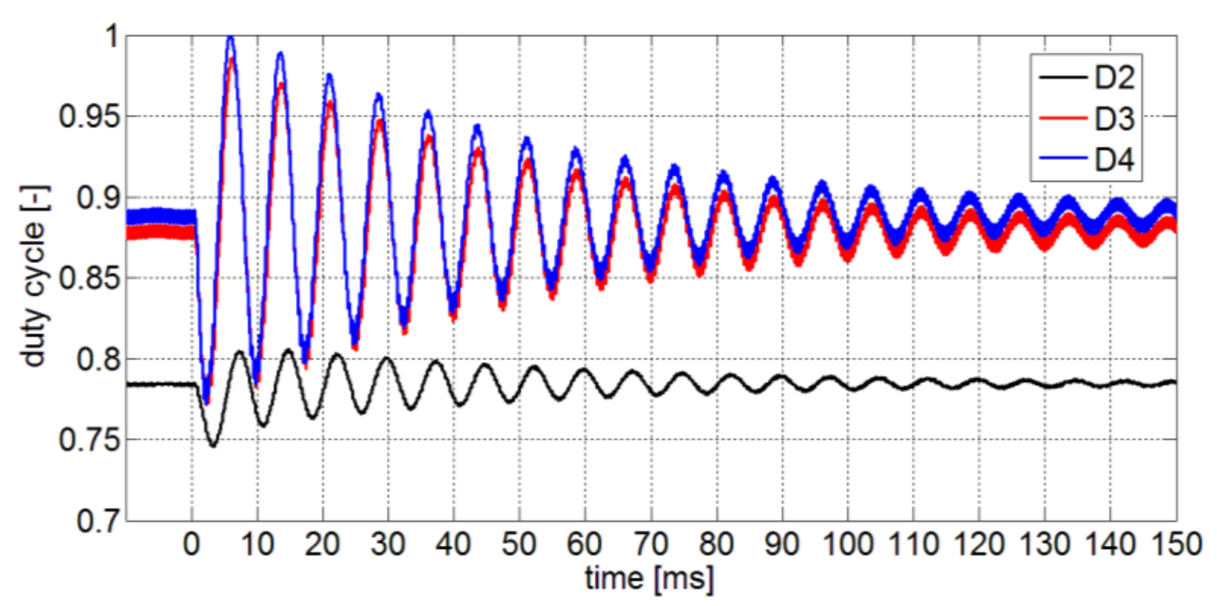
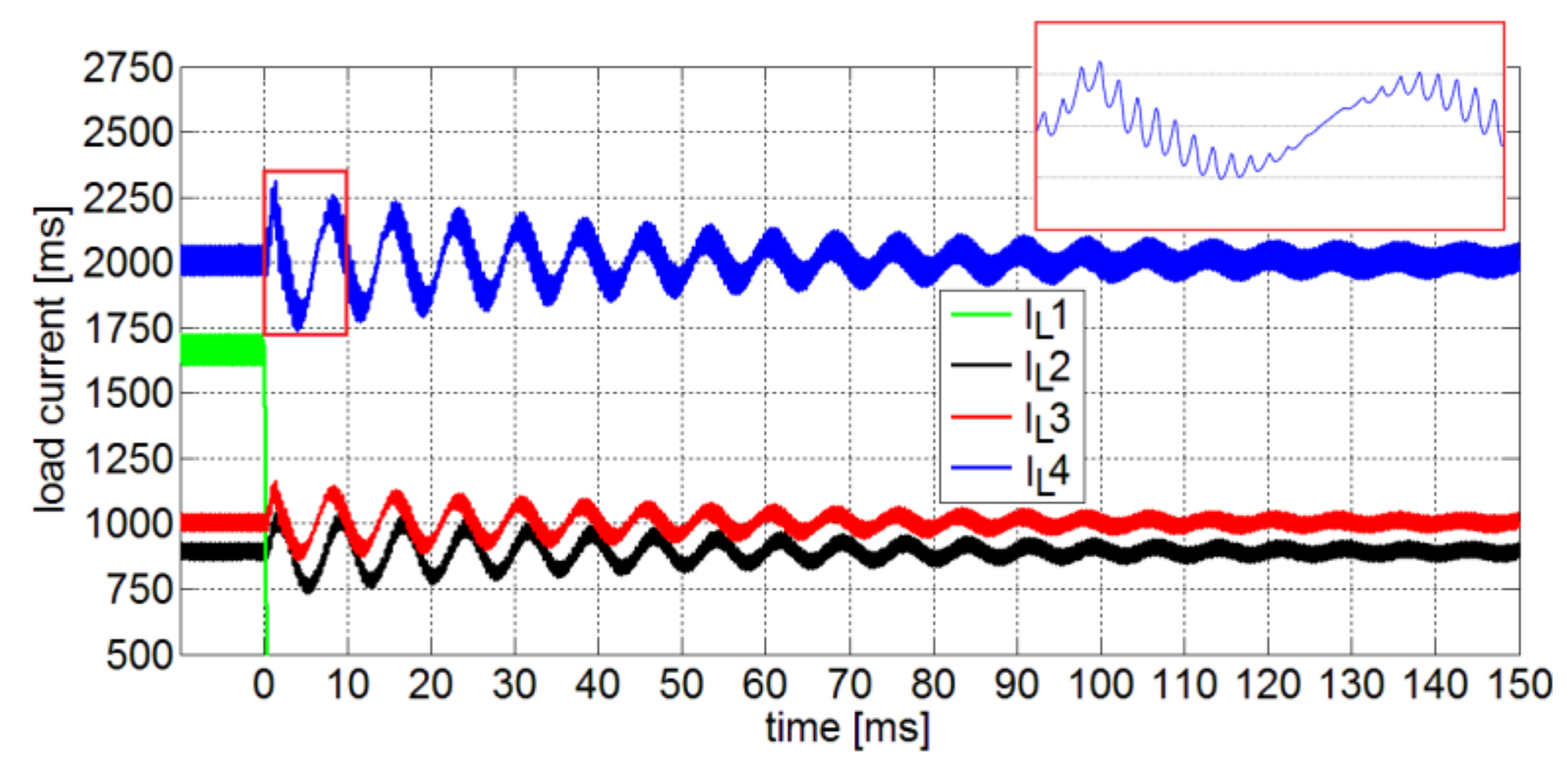
To prove the validity of the WBM stability assessment, a DC shipboard system with four voltage-controlled DC-DC converters (Table 1) is emulated by Typhoon HIL 604 real-time platform (Figure 8). The controlled DC grid is modeled by means of the Software-In-the-Loop approach, thus the system-control code is compiled to run real-time simulation where the detailed switching behavior is made visible. The four controlled DC-DC converters are synthesized in HIL schematic editor (Figure 8), where core coupling elements subdivide the numerical task in three cores. In such a way, the platform can offer real-time transients notwithstanding the small simulation time step (0.5 μs). In the HIL tests, a perturbation (i.e., disconnection of load 1) is applied at t = 0 s to establish the analyzed scenarios. First, the instability of Case 1 (Ψ = 1.18) results evident in Figure 9, where the bus voltage presents a limit cycle (range of ±17%) thus forcing the consequent intervention of protections. Conversely, the best stability performance (Ψ = 0.65) is highlighted in the Case 3 results (Figure 10, Figure 11, Figure 12, Figure 13 and Figure 14), confirming the stability assessment. Although the stability analysis disregards the presence of load filters, it results coherent with emulations, which on the contrary also considered the filtering stages. The control validity is confirmed on the bus voltage transient (Figure 10), where the rated value (6000 V) is restored in about 150 ms by an underdamped evolution. In a steady state condition, the peak-peak voltage ripple ΔV% results equal to 4% thus in accordance to the requirements in [9]. The controlled load voltages in Figure 11 also display a well-filtered behavior as the LC components on loads are sized to ensure ΔV% = 7%. Regarding the actuators, Figure 12 shows the duty cycle signals to impose a stable steady state condition on the bus voltage, while avoiding the saturation (i.e., Y-axis = 1). When the dynamics transient is concluded in t > 150 ms, the final duty values are greater than the rated Dnk (Table 1) to compensate for the voltage drop on filter resistances Rfk. The converter’s currents are in Figure 13 while Figure 14 shows the loads currents. In both transients, a settling time of 150 ms is visible. The currents in the filter inductors (Figure 13) exhibit ripples (ΔI% < 30%) in compliance with the desired power quality (Table 1), conversely smaller ripples (ΔI% ≈ 4%) are visible on loads currents (Figure 14).
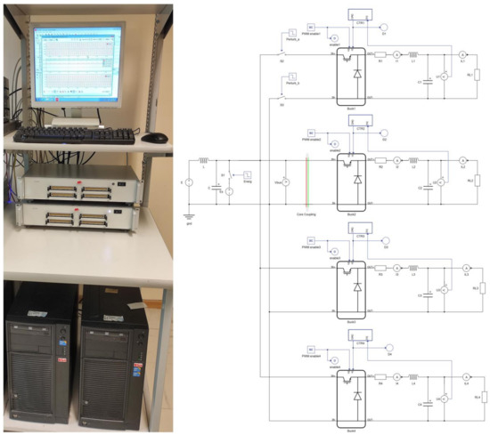
Figure 8.
Typhoon HIL 604 real-time platform (photo on the left) to implement the controlled power converters (schematic editor on the right).
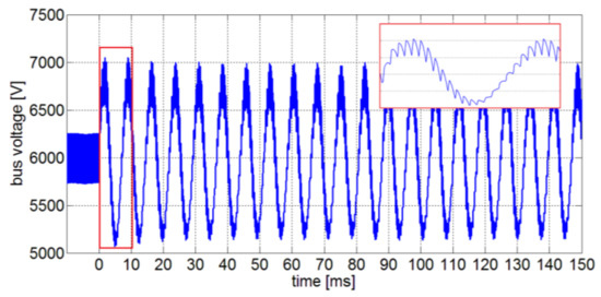
Figure 9.
Bus voltage transient in Case 1 (each Y-division is 500 V in zoomed graph).
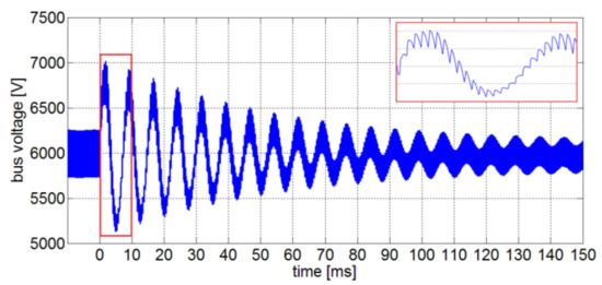
Figure 10.
Bus voltage transient in Case 3 (each Y-division is 500 V in zoomed graph).
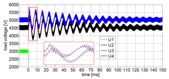
Figure 11.
Load voltages transient in Case 3 (each Y-division is 500 V in zoomed graph).

Figure 12.
Duty cycles transient in Case 3.
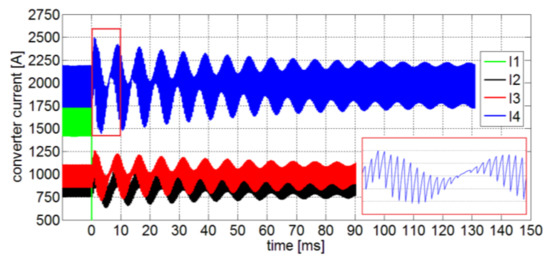
Figure 13.
Converter currents transient in Case 3 (each Y-division is 250 A in zoomed graph).

Figure 14.
Load currents transient in Case 3 (each Y-division is 250 A in zoomed graph).
5.5. Considerations on Stability Assessment and HIL Results
The results and figures of this paper are able to demonstrate the potentiality of the proposed approach. First, the Nyquist diagram in Figure 5 can provide an interesting overview about the stability performance of the three cases (i.e., three bandwidths combination) under study. When the perturbation affects the power grid in Case 1, the intersection in −1.18 means instability. Different scenarios are visible in the other two cases, where the reductions in bandwidths are able to restore the system stability even after the perturbation. Then, Figure 6 and Figure 7 are crucial because they confirm the WBM model, named SD, as less conservative. Indeed, the related complex poles (red) are always on the right of the initial complex poles (blue). This means that the aggregated model is more inclined to instability. If the multiconverter control is designed to maintain the aggregated poles on the left plane, certainly also the poles of initial complex system are on the left, thus representative of stable evolutions. Finally, Figure 9, Figure 10, Figure 11, Figure 12, Figure 13 and Figure 14 show the real-time behavior by implementing the Typhoon HIL emulation. These transients are important because they validate the previous consideration: when the control bandwidths are not harmonized as in Case 1, the instability is consequent as in Figure 9. Differently, when the iterative process is applied on the WBM aggregated model, a convenient reduction in bandwidths is the solution for achieving the stability, even after the perturbation. This stable performance is made evident in the bus voltage transient of Figure 10, as well as in all the other transients, from Figure 11, Figure 12, Figure 13 and Figure 14.
6. Conclusions
The system stability is an important requirement in shipboard MVDC power systems, where undesired voltage oscillations can lead to blackouts. In this context, the paper has studied a methodology to assess system stability in a radial multiple-loads DC grid. As DC shipboard systems are complex (i.e., tens/hundreds controlled loads), some assumptions (e.g., load filters disregarding) are initially established to simplify the modeling while identifying the range of validity. Since a low-bandwidth controlled converter can balance the destabilizing action of a high-performance converter, WBM is proposed to aggregate the multiple controlled loads in the two stabilizing/destabilizing sets. Once WBM is proved to be less conservative, load aggregation is the base on which the iterative process for the stability assessment is developed. By taking into account the compensation provided by low-performance converters, attention is spent on the stability criterion’s verification. In particular, the reduction on bandwidths results effective in reestablishing the DC stability, if the destabilizing load quota is hypothetically known from the electrical balance or Power Management System. In order to test the weighted bandwidth method, a DC shipboard power system consisting of four controlled converters is used as the study case on which to evaluate the effects of control bandwidths on system stability. Although the methodology is conceived on a DC system with a limited number of controlled loads, the results are directly transferable to a realistic DC shipboard grid, thus the study contributes with high engineering value. Finally, HIL emulations test the preemptive stability assessments by verifying the restoration of stable evolutions towards equilibrium points.
Author Contributions
Conceptualization, D.B. and G.G.; methodology, D.B. and G.S.; software, D.B. and S.P.; validation, D.B.; formal analysis, D.B. and G.G.; investigation, D.B., G.G., S.P. and G.S.; resources, D.B. and G.G.; data curation, D.B.; writing—original draft preparation, D.B. and G.G.; writing—review and editing, D.B., G.G., S.P. and G.S.; visualization, D.B.; supervision, G.S. All authors have read and agreed to the published version of the manuscript.
Funding
This research received no external funding.
Institutional Review Board Statement
Not applicable.
Informed Consent Statement
Not applicable.
Data Availability Statement
Data available on request due to restrictions.
Acknowledgments
The authors would like to thank Typhoon HIL for providing the platform used in the development of this research work.
Conflicts of Interest
The authors declare no conflict of interest.
References
- Dragicevic, T.; Vasquez, J.C.; Guerrero, J.; Škrlec, D. Advanced LVDC Electrical Power Architectures and Microgrids: A step toward a new generation of power distribution networks. IEEE Electrif. Mag. 2014, 2, 54–65. [Google Scholar] [CrossRef] [Green Version]
- Zubieta, L.E. Are Microgrids the Future of Energy? DC Microgrids from Concept to Demonstration to Deployment. IEEE Electrif. Mag. 2016, 4, 37–44. [Google Scholar] [CrossRef]
- Wang, F.; Zhang, Z.; Ericsen, T.; Raju, R.; Burgos, R.; Boroyevich, D. Advances in Power Conversion and Drives for Shipboard Systems. Proc. IEEE 2015, 103, 2285–2311. [Google Scholar] [CrossRef]
- Chen, Y.; Li, Z.; Zhao, S.; Wei, X.; Kang, Y. Design and Implementation of a Modular Multilevel Converter with Hierarchical Redundancy Ability for Electric Ship MVDC System. IEEE J. Emerg. Sel. Top. Power Electron. 2017, 5, 189–202. [Google Scholar] [CrossRef]
- Lemmon, A.N.; Graves, R.C.; Kini, R.L.; Hontz, M.R.; Khanna, R. Characterization and Modeling of 10-kV Silicon Carbide Modules for Naval Applications. IEEE J. Emerg. Sel. Top. Power Electron. 2017, 5, 309–322. [Google Scholar] [CrossRef]
- Javaid, U.; Freijedo, F.D.; Dujic, D.; van der Merwe, W. MVDC supply technologies for marine electrical distribution systems. CPSS Trans. Power Electron. Appl. 2018, 3, 65–76. [Google Scholar] [CrossRef]
- Islam, M.M. Shipboard Power System with LVDC and MVDC for AC and DC Application. In VFD Challenges for Shipboard Electrical Power System Design; IEEE: Piscataway, NJ, USA, 2019; pp. 35–37. [Google Scholar]
- Moore, T.J.; Richardson, J.M.; Markle, S.P. NPES Technology Development Roadmap. Naval Sea Systems Command. 2019. Available online: https://news.usni.org/2019/06/26/u-s-naval-power-and-energy-systems-technology-development-roadmap (accessed on 22 November 2021).
- IEEE Standards Association. IEEE Recommended Practice for 1 kV to 35 kV Medium-Voltage DC Power Systems on Ships; IEEE Std 1709-2018 (Revision of IEEE Std 1709–2010); IEEE: Piscataway, NJ, USA, 2018; pp. 1–54. [Google Scholar]
- Cuzner, R.M.; Soman, R.; Steurer, M.M.; Toshon, T.A.; Faruque, M.O. Approach to Scalable Model Development for Navy Shipboard Compatible Modular Multilevel Converters. IEEE J. Emerg. Sel. Top. Power Electron. 2017, 5, 28–39. [Google Scholar] [CrossRef]
- Soman, R.; Steurer, M.M.; Toshon, T.A.; Faruque, M.O.; Cuzner, R.M. Size and Weight Computation of MVDC Power Equipment in Architectures Developed Using the Smart Ship Systems Design Environment. IEEE J. Emerg. Sel. Top. Power Electron. 2017, 5, 40–50. [Google Scholar] [CrossRef]
- Sudhoff, S.; Corzine, K.; Glover, S.; Hegner, H.; Robey, H. DC link stabilized field oriented control of electric propulsion systems. IEEE Trans. Energy Convers. 1998, 13, 27–33. [Google Scholar] [CrossRef]
- Sudhoff, S.D.; Glover, S.F.; Lamm, P.T.; Schmucker, D.H.; Delisle, D.E. Admittance space stability analysis of power electronic systems. IEEE Trans. Aerosp. Electron. Syst. 2000, 36, 965–973. [Google Scholar] [CrossRef]
- Wang, C.; Duan, J.; Fan, B.; Yang, Q.; Liu, W. Decentralized High-Performance Control of DC Microgrids. IEEE Trans. Smart Grid 2019, 10, 3355–3363. [Google Scholar] [CrossRef]
- Rivetta, C.H.; Emadi, A.; Williamson, G.A.; Jayabalan, R.; Fahimi, B. Analysis and control of a buck DC-DC converter operating with constant power load in sea and undersea vehicles. IEEE Trans. Ind. Appl. 2006, 42, 559–572. [Google Scholar] [CrossRef]
- Kwasinski, A.; Onwuchekwa, C.N. Dynamic Behavior and Stabilization of DC Microgrids with Instantaneous Constant-Power Loads. IEEE Trans. Power Electron. 2011, 26, 822–834. [Google Scholar] [CrossRef]
- Cupelli, M.; Ponci, F.; Sulligoi, G.; Vicenzutti, A.; Edrington, C.S.; El-Mezyani, T.; Monti, A. Power Flow Control and Network Stability in an All-Electric Ship. Proc. IEEE 2015, 103, 2355–2380. [Google Scholar] [CrossRef] [Green Version]
- Dragicevic, T.; Lu, X.; Vasquez, J.C.; Guerrero, J.M. DC Microgrids—Part I: A Review of Control Strategies and Stabilization Techniques. IEEE Trans. Power Electron. 2016, 31, 4876–4891. [Google Scholar] [CrossRef] [Green Version]
- Herrera, L.; Zhang, W.; Wang, J. Stability Analysis and Controller Design of DC Microgrids with Constant Power Loads. IEEE Trans. Smart Grid 2017, 8, 881–888. [Google Scholar]
- Huangfu, Y.; Pang, S.; Nahid-Mobarakeh, B.; Guo, L.; Rathore, A.K.; Gao, F. Stability Analysis and Active Stabilization of On-board DC Power Converter System with Input Filter. IEEE Trans. Ind. Electron. 2018, 65, 790–799. [Google Scholar] [CrossRef]
- Potty, K.A.; Bauer, E.; Li, H.; Wang, J. Smart Resistor: Stabilization of DC Microgrids Containing Constant Power Loads Using High-Bandwidth Power Converters and Energy Storage. IEEE Trans. Power Electron. 2020, 35, 957–967. [Google Scholar] [CrossRef]
- Pakdeeto, J.; Areerak, K.; Bozhko, S.; Areerak, K. Stabilization of DC MicroGrid Systems by Using the Loop-Cancellation Technique. IEEE J. Emerg. Sel. Top. Power Electron. 2021, 9, 2652–2663. [Google Scholar] [CrossRef]
- Sulligoi, G.; Bosich, D.; Giadrossi, G.; Zhu, L.; Cupelli, M.; Monti, A. Multiconverter Medium Voltage DC Power Systems on Ships: Constant-Power Loads Instability Solution Using Linearization via State Feedback Control. IEEE Trans. Smart Grid 2014, 5, 2543–2552. [Google Scholar] [CrossRef]
- Bosich, D.; Sulligoi, G.; Mocanu, E.; Gibescu, M.M. Medium Voltage DC Power Systems on Ships: An Offline Parameter Estimation for Tuning the Controllers’ Linearizing Function. IEEE Trans. Energy Convers. 2017, 32, 748–758. [Google Scholar] [CrossRef]
- Cupelli, M.; Zhu, L.; Monti, A. Why Ideal Constant Power Loads Are Not the Worst Case Condition From a Control Standpoint. IEEE Trans. Smart Grid 2015, 6, 2596–2606. [Google Scholar] [CrossRef] [Green Version]
- Magne, P.; Nahid-Mobarakeh, B.; Pierfederici, S. Dynamic Consideration of DC Microgrids with Constant Power Loads and Active Damping System—A Design Method for Fault-Tolerant Stabilizing System. IEEE J. Emerg. Sel. Top. Power Electron. 2014, 2, 562–570. [Google Scholar] [CrossRef]
- Alacano, A.; Valera, J.J.; Abad, G.; Izurza, P. Power-Electronic-Based DC Distribution Systems for Electrically Propelled Vessels: A Multivariable Modeling Approach for Design and Analysis. IEEE J. Emerg. Sel. Top. Power Electron. 2017, 5, 1604–1620. [Google Scholar] [CrossRef]
- Javaid, U.; Freijedo, F.D.; Dujic, D.; Van Der Merwe, W. Dynamic Assessment of Source—Load Interactions in Marine MVDC Distribution. IEEE Trans. Ind. Electron. 2017, 64, 4372–4381. [Google Scholar] [CrossRef]
- Javaid, U.; Freijedo, F.D.; Van Der Merwe, W.; Dujic, D. Stability Analysis of Multi-Port MVDC Distribution Networks for All-Electric Ships. IEEE J. Emerg. Sel. Top. Power Electron. 2020, 8, 1164–1177. [Google Scholar] [CrossRef]
- Pastore, S.; Bosich, D.; Sulligoi, G. Analysis of small-signal voltage stability for a reduced-order cascade-connected MVDC power system. In Proceedings of the IECON 2017—43rd Annual Conference of the IEEE Industrial Electronics Society, Beijing, China, 29 October–1 November 2017; pp. 6771–6776. [Google Scholar]
- Pastore, S.; Bosich, D.; Sulligoi, G. A frequency analysis of the small-signal voltage model of a MVDC power system with two cascade DC-DC converters. In Proceedings of the 2018 IEEE International Conference on Electrical Systems for Aircraft, Railway, Ship Propulsion and Road Vehicles & International Transportation Electrification Conference (ESARS-ITEC), Nottingham, UK, 7–9 November 2018; pp. 1–6. [Google Scholar]
- Chalfant, J. Early-Stage Design for Electric Ship. Proc. IEEE 2015, 103, 2252–2266. [Google Scholar] [CrossRef]
- Ericsen, T. The Second Electronic Revolution (It’s All about Control). In Proceedings of the 2009 Record of Conference Papers-Industry Applications Society 56th Annual Petroleum and Chemical Industry Conference, Anaheim, CA, USA, 14–16 September 2009; Volume 46, pp. 1778–1786. [Google Scholar]
- Sulligoi, G.; Bosich, D.; Vicenzutti, A.; Khersonsky, Y. Design of Zonal Electrical Distribution Systems for Ships and Oil Platforms: Control Systems and Protections. IEEE Trans. Ind. Appl. 2020, 56, 5656–5669. [Google Scholar] [CrossRef]
- Du, W.; Fu, Q.; Wang, H.F. Small-Signal Stability of a DC Network Planned for Electric Vehicle Charging. IEEE Trans. Smart Grid 2020, 11, 3748–3762. [Google Scholar] [CrossRef]
- Feng, X.; Ye, Z.; Xing, K.; Lee, F.; Borojevic, D. Individual load impedance specification for a stable DC distributed power system. In Proceedings of the APEC’99. Fourteenth Annual Applied Power Electronics Conference and Exposition. 1999 Conference Proceedings (Cat. No. 99CH36285), Dallas, TX, USA, 14–18 March 1999; Volume 2, pp. 923–929. [Google Scholar]
- Riccobono, A.; Santi, E. Comprehensive Review of Stability Criteria for DC Power Distribution Systems. IEEE Trans. Ind. Appl. 2014, 50, 3525–3535. [Google Scholar] [CrossRef]
- Siegers, J.; Arrua, S.; Santi, E. Stabilizing Controller Design for Multibus MVdc Distribution Systems Using a Passivity-Based Stability Criterion and Positive Feedforward Control. IEEE J. Emerg. Sel. Top. Power Electron. 2017, 5, 14–27. [Google Scholar] [CrossRef]
- Riccobono, A.; Cupelli, M.; Monti, A.; Santi, E.; Roinila, T.; Abdollahi, H.; Arrua, S.; Dougal, R.A. Stability of Shipboard DC Power Distribution: Online Impedance-Based Systems Methods. IEEE Electrif. Mag. 2017, 5, 55–67. [Google Scholar] [CrossRef]
- Rygg, A.; Molinas, M. Apparent Impedance Analysis: A Small-Signal Method for Stability Analysis of Power Electronic-Based Systems. IEEE J. Emerg. Sel. Top. Power Electron. 2017, 5, 1474–1486. [Google Scholar] [CrossRef] [Green Version]
- Zhang, X.; Ruan, X.; Tse, C. Impedance-Based Local Stability Criterion for DC Distributed Power Systems. IEEE Trans. Circuits Syst. I Regul. Pap. 2015, 62, 916–925. [Google Scholar] [CrossRef]
- Amin, M.; Molinas, M. Small-Signal Stability Assessment of Power Electronics Based Power Systems: A Discussion of Impedance- and Eigenvalue-Based Methods. IEEE Trans. Ind. Appl. 2017, 53, 5014–5030. [Google Scholar] [CrossRef]
- Su, M.; Liu, Z.; Sun, Y.; Han, H.; Hou, X. Stability Analysis and Stabilization Methods of DC Microgrid With Multiple Parallel-Connected DC–DC Converters Loaded by CPLs. IEEE Trans. Smart Grid 2018, 9, 132–142. [Google Scholar] [CrossRef]
- IEEE Standards Association. IEEE Std 141--1993; IEEE Recommended Practice for Electric Power Distribution for Industrial Plants. IEEE: Piscataway, NJ, USA, 1994; pp. 1–768.
- Oh, C.-H.; Go, S.-I.; Choi, J.-H.; Ahn, S.-J.; Yun, S.-Y. Voltage Estimation Method for Power Distribution Networks Using High-Precision Measurements. Energies 2020, 13, 2385. [Google Scholar] [CrossRef]
- Park, J.; Lee, S.Y.; Park, P. A Less Conservative Stability Criterion for Discrete-Time Lur’e Systems with Sector and Slope Restrictions. IEEE Trans. Autom. Control 2019, 64, 4391–4395. [Google Scholar] [CrossRef]
- Lin, C.; Wang, Q.C.; Lee, T.H. A less conservative robust stability test for linear uncertain time-delay systems. IEEE Trans. Autom. Control 2006, 51, 87–91. [Google Scholar] [CrossRef]


Publisher’s Note: MDPI stays neutral with regard to jurisdictional claims in published maps and institutional affiliations. |
© 2021 by the authors. Licensee MDPI, Basel, Switzerland. This article is an open access article distributed under the terms and conditions of the Creative Commons Attribution (CC BY) license (https://creativecommons.org/licenses/by/4.0/).