Article

Nonlinear Modeling of Dynamic Characteristics of Pump-Turbine

School of Water Conservancy and Hydropower, Hebei University of Engineering, Handan 056038, China
*
Author to whom correspondence should be addressed.
Energies 2022, 15(1), 297; https://doi.org/10.3390/en15010297
Submission received: 6 November 2021 / Revised: 25 December 2021 / Accepted: 30 December 2021 / Published: 2 January 2022
(This article belongs to the Section A: Sustainable Energy)

Abstract

:
Hydropower is a kind of clean energy, which can effectively reduce the consumption of fossil energy and is one of the main fields of new energy development. Pumped storage power station not only provides a solution for storing electric energy and generating excess, but also is a clean, efficient, economical and safe power system regulation method with high quality. Accurate modeling of a pump-turbine, as the core equipment of a pumped storage unit, is the key to safe and stable operation of the pumped storage unit. At present, a method of simplifying the external characteristics of a pump-turbine into a first-order linear model is widely used, which cannot effectively and accurately reveal the nonlinear dynamic characteristics of the unit in transition process. In order to meet the demand of high-precision simulation of the unit, a new method of identifying Taylor series expansion considering nonlinearity based on the torque characteristic formula and the flow characteristic formula is proposed, which is applied to the pump-turbine external characteristic model, and retains the second derivative term, making the model a second-order nonlinear model, and thus, the pump-turbine model becomes a nonlinear model. The nonlinear model established is used to simulate the load increase and load rejection of the unit, and the results are compared with those for the linear model. The comparison shows that the nonlinear model established for the pump-turbine can reveal the dynamic response of the unit more effectively and accurately than the linear model, and provide a further guarantee for the safe and stable operation of pumped-storage units, which is of great significance to hydropower energy development.

1. Introduction

A pump-turbine is the core component of a pumped storage unit [1], and its dynamic characteristics play a decisive role in the stability of a hydropower station [2,3,4,5,6]. Therefore, accurate modeling of the pump-turbine is particularly important for the stability of the hydropower station’s governing system. The dynamic relationship between various operating variables of the pump-turbine is very complicated [7,8,9]. In general, the dynamic characteristics of the pump-turbine are often expressed by torque characteristics and flow characteristics under steady-state conditions [9,10]. Usually, Taylor expansion is carried out on the torque and flow formulas, and the second-order and higher-order derivative terms are omitted, so that they become linear models. At present, the first-order linear model of pump-turbine is widely used. Xu. et al. [11] and Liu. et al. [12] combined the linear model of pump-turbine to build the mathematical model of pump-turbine regulation. By combining the linear model of pump-turbine, Zhou, J. et al. [13] proposed an online simulation method of two iterative loops composed of improved Sutter transform and neural network, which improved the solution accuracy of pump-turbine. Although the linear model is simple and easy to solve, it cannot truly and accurately describe the pump-turbine’s characteristics [9,14,15]. In view of this, the model is improved in this paper in order to describe the dynamic characteristics of the pump-turbine more accurately and effectively. On the basis of previous studies, Taylor expansion is carried out on the formulas of flow characteristics and moment characteristics, retaining the second derivative term and ignoring the third and higher derivative terms, which make the model become a more accurate nonlinear model.
The complete characteristic curve of a pump-turbine in China was obtained according to the measured data, and the transfer coefficient of the first-order partial derivative in the mathematical model for the pump-turbine was obtained by using the external characteristic method. Based on the established nonlinear mathematical model for the pump-turbine and the complete speed regulation system model of a pumped storage unit [16,17,18], the established speed regulation system was simulated [19].
The time domain simulation is a common method to analyze the stability of nonlinear systems. The accuracy of transient stability analysis by the time domain simulation method is closely related to the numerical calculation method selected. The Euler method has low accuracy and poor numerical stability; the Runge–Kutta method fits the higher-order terms of Taylor series, which has high accuracy and good numerical stability. The linear multi-step method has high accuracy, and the calculation amount is smaller than that of Runge–Kutta method, but the calculation result is greatly influenced by the initial value, so it is necessary to choose an appropriate starting algorithm to ensure its accuracy [20]. Therefore, this paper adopts the time domain simulation combined with Longge-Kutafa, which has higher accuracy. The phase plane method is an analysis method based on the time domain. This method transforms the motion process of the first-order and second-order systems into the phase trajectory on the position and velocity plane by the graphic method, which can reflect the stability, equilibrium state and steady-state accuracy of the system, and the influence of initial conditions and parameters on the system motion intuitively and accurately [21]. Therefore, in the simulation of the system in this paper, both the traditional one-dimensional time domain response diagram and the intuitive phase trajectory diagram are used. The dynamic response process of the pump-turbine was studied by using the nonlinear dynamic characteristics such as time domain diagram and phase trajectory diagram obtained from simulation [22,23,24,25,26]. By comparing and analyzing the dynamic responses for linear model and nonlinear model under load disturbance [27,28,29,30], the dynamic change law and characteristics of the system are further analyzed, which provides theoretical basis and scientific guidance for further research on nonlinear model of pump-turbine [9].

2. Constructing the Mathematical Model for Pump-Turbine Governing System

2.1. Pump-Turbine Model

2.1.1. Research Method of Mathematical Model of Hydraulic Turbine

The establishment of a mathematical model for a hydraulic turbine generally has the following steps. First, the model is established by using the internal characteristics method of hydraulic turbine. The internal characteristics of hydraulic turbine are the internal flow laws and the structural parameters of hydraulic turbine. So, an internal characteristic model corresponding to a hydraulic turbine is established according to the physical principle for the hydraulic turbine itself [9,14,31,32]. Second, the model is established according to the numerical method of external characteristics of hydraulic turbine. The numerical solution method for the external characteristics of the hydraulic turbine is to obtain the full characteristics curve of the hydraulic turbine through the mathematical methods such as interpolation and fitting based on the limited comprehensive characteristics data of the hydraulic turbine. By this method, the mathematical model of the comprehensive characteristic curve for the hydraulic turbine, which takes the comprehensive characteristic curve for the hydraulic turbine as the boundary condition of the numerical characteristic of the hydraulic turbine, is established [9,14,31,32]. Third, the nonlinear water turbine model is proposed by IEEE PES Working Group on Prime Mover [33,34].
Based on the mathematical model formula of the comprehensive characteristic curve for the turbine, under the steady-state working condition of the turbine, the flow characteristic equation and the moment characteristic equation were extended to Taylor series, a nonlinear model containing second derivative was obtained with the second derivative term being retained, and the third-order and higher-order trace being ignored.

2.1.2. Derivation of Nonlinear Model of Pump-Turbine

The torque characteristics and flow characteristics of the dynamic characteristics of hydraulic turbines under steady-state conditions can be expressed as [7,9,14,28,35,36]:
M t = M t ( a , n , H ) ,
Q = Q ( a , n , H ) ,
where Mt is the pump-turbine torque, Q is the pump-turbine flow rate, a is the guide vane opening, n is the pump-turbine speed, and H is the pump-turbine working head. In the case of small fluctuations, the initial operating point of the turbine is set to a = a0 +a, n = n0 +n, H = H0 +H. The torque characteristics and flow characteristics represented by the implicit functions in Equations (1) and (2) are extended to Taylor series at the operating point, respectively, and the following results are obtained:
Δ M t = M t ( a , n , H ) M t ( a 0 , n 0 , H 0 ) = M t a Δ a + M t n Δ n + M t H Δ H + 2 M t a 2 Δ a 2 2 + 2 M t n 2 Δ n 2 2 + 2 M t H 2 Δ H 2 2 + 2 [ 2 M t a n Δ a Δ n 2 + 2 M t a H Δ a Δ H 2 + 2 M t n H Δ n Δ H 2 ] = M t a Δ a + M t n Δ n + M t H Δ H + 2 M t a 2 Δ a 2 2 + 2 M t n 2 Δ n 2 2 + 2 M t H 2 Δ H 2 2 + 2 M t a n Δ a Δ n + 2 M t a H Δ a Δ H + 2 M t n H Δ n Δ H ,
Δ Q = Q ( a , n , H ) Q ( a 0 , n 0 , H 0 ) = Q a Δ a + Q n Δ n + Q H Δ H + 2 Q a 2 Δ a 2 2 + 2 Q n 2 Δ n 2 2 + 2 Q H 2 Δ H 2 2 + 2 Q a n Δ a Δ n + 2 Q a H Δ a Δ H + 2 Q n H Δ n Δ H ,
where m t = Δ M t / M r , is the relative value of torque deviation, q = Δ Q / Q r is the relative value of flow deviation, y = Δ a / a max is the relative value of the guide vane opening deviation, x = Δ n / n r is the relative value of speed deviation, and h = Δ H / H r is the relative value of head deviation. Then there are:
m t = M t M r a a max y + M t M r n n r x + M t M r H H r h + 1 2 [ 2 ( M t M r ) ( a a max ) 2 y 2 + 2 ( M t M r ) ( n n r ) 2 x 2 + 2 ( M t M r ) ( H H r ) 2 h 2 ] + [ 2 ( M t M r ) ( a a max ) ( n n r ) y x + 2 ( M t M r ) ( a a max ) ( H H r ) y h + 2 ( M t M r ) ( H H r ) ( n n r ) x h ] ,
That is:
m t = m t y y + m t x x + m t h h + 1 2 [ 2 ( m t ) ( y ) 2 y 2 + 2 ( m t ) ( x ) 2 x 2 + 2 ( m t ) ( h ) 2 h 2 ] + [ 2 ( m t ) y x y x + 2 ( m t ) y h y h + 2 ( m t ) h x x h ] ,
q = Q Q r a a max y + Q Q r n n r x + Q Q r H H r h + 1 2 [ 2 ( Q Q r ) ( a a max ) 2 y 2 + 2 ( Q Q r ) ( n n r ) 2 x 2 + 2 ( Q Q r ) ( H H r ) 2 h 2 ] + [ 2 ( Q Q r ) ( a a max ) ( n n r ) y x + 2 ( Q Q r ) ( a a max ) ( H H r ) y h + 2 ( Q Q r ) ( H H r ) ( n n r ) x h ] ,
That is:
q = q y y + q x x + q h h + 1 2 [ 2 q ( y ) 2 y 2 + 2 q ( x ) 2 x 2 + 2 q ( h ) 2 h 2 ] + [ 2 q y x y x + 2 q y h y h + 2 q h x x h ] ,
Let:
e h = m t h , e x = m t x , e y = m t y , e y y = 2 ( m t ) y 2 , e x x = 2 ( m t ) x 2 , e h h = 2 ( m t ) h 2 , e q h = q h , e q x = q x , e q y = q y , e y x = 2 ( m t ) y x , e y h = 2 ( m t ) y h , e x h = 2 ( m t ) h x , e q y y = 2 q y 2 , e q x x = 2 q x 2 , e q h h = 2 q h 2 , e q y x = 2 q y x , e q y h = 2 q y h , e q x h = 2 q h x . where ex is the transmission coefficient of torque to rotational speed, ey is the relative coefficient of moment to guide vane opening, eh is the transfer coefficient of torque to working head, eqx is the relative coefficient of flow to rotational speed, eqh is the relative coefficient of flow to working head, and eqy is the relative coefficient of flow to guide vane opening [37].
Then, the nonlinear model of the pump-turbine is derived as:
m t = e y y + e x x + e h h + 1 2 [ e y y y 2 + e x x x 2 + e h h h 2 ] + e y x y x + e y h y h + e x h x h ,
q = e q y y + e q x x + e q h h + 1 2 [ e q y y y 2 + e q x x x 2 + e q h h h 2 ] + e q y x y x + e q y h y h + e q x h x h

2.2. Generator Model

The hydraulic turbine and the generator are connected by the main shaft as a whole. Its rotating part can be regarded as a rigid system rotating around a fixed axis. The motion equation of the hydraulic turbine generator set is [38]:
J d ω d t = M t M g ,
where J is the moment of inertia of the rotating part of the unit and J = G D 2 / 4 g , G D 2 is the flywheel moment of hydraulic turbine unit, g is the acceleration due to gravity, ω is the angular velocity of the unit rotation and ω = 2 π n / 60 , Mt is the driving torque of hydraulic turbine, and Mg is the resistance torque of the generator.
The initial stable condition of the system was set to t = 0 , ω = 2 π n / 60 , and M t = M t 0 = M g = M g 0 . When t > 0 , when the governing system is switched to a dynamic process, we can get ω = ω 0 + Δ ω , M t = M t 0 + Δ M t , M g = M g 0 + Δ M g , and substituting them into the Formula (11), we can obtain:
J d Δ ω d t = Δ M t Δ M g ,
The rated torque M r is taken as the reference value of Δ M t and Δ M g , and the rated angular velocity ω r is taken as the reference value of Δ ω . m t = Δ M t / M r , m g = Δ M g / M r , and x = Δ ω / ω r are respectively expressed as the relative values of driving torque, load torque, and rotational speed deviation. So, Equation (12) is transformed as:
T a d x d t = m t m g ,
where T a = J ω r / M r , Ta are inertia time constants of the unit, and their physical meaning is: the time for the unit to accelerate from zero to the rated speed with the rated torque.
The relative value of load moment deviation of the generator set from initial stable working condition to the dynamic process of the governing system is:
m g = e g x + m g 0 ,   e g = i = 1 n d M g i M r d ω ω r ,
where eg is the load self-adjusting coefficient of the generator, which is used to express the change rate of the load torque of the generator with the rotating speed, and the range of its values is eg > 0. mg0 represents the load torque at t = 0 , which does not change with the speed, and mg0 is the disturbance torque of the governing system.
Substituting Equation (14) into Equation (13), we can get:
T a d x d t = m t m g 0 e g x .

2.3. Diversion Pipeline Model

The dynamic equation of pressure pipeline [39] is expressed as:
T w 0 d q d t = h ,
where Tw0 is the inertia time constant of pressure pipeline water flow.

2.4. Governor Equation

The governor equation is selected as [38]:
d y d t = K p d x d t K i x ,
where Kp and Ki represent the proportional and integral coefficients.
Combining Equations (9), (10) and (15)–(17), the state space equations of the system are obtained as:
x ˙ = 1 T a [ A x + B y + C h m g ] ,
y ˙ = K p T a [ ( A + T a K i K p ) x + B y + C h m g ] ,
h ˙ = x [ A E ( f y y + f x x + f h h + f c ) + T a K i E ( e q y + e q y y y + e q x y x + e q y h h ) ] + y B E ( f y y + f x x + f h h + f c ) + h T a + T w 0 C ( f y y + f x x + f h h + f c ) E T w 0 m g E ( f y y + f x x + f h h + f c ) ,
where, A = e x e g + e x y y + e x h h + 1 2 e x x x , B = e y + e y h h + 1 2 e y y y , C = e h + 1 2 e h h h , E = T a ( e q h + e q y h y + e q x h x + e q h h h ) , f x = K p e q x y e q x x , f y = K p e q y y e q y x , f h = K p e q y h e q x h , f c = K p e q y e q x .
The above formula is the state space equation established by the pump-turbine governing system based on the pump-turbine nonlinear model.

3. Obtaining the Transfer Coefficient for Pump-Turbine in Generating Mode

3.1. Calculation Method of Transfer Coefficient for Pump-Turbine

In the mathematical model for the pump-turbine, the coefficients ex, ey, eh, eqx, eqh, and eqy of the first-order partial derivative are usually called the transfer coefficients of the pump-turbine. The transfer coefficients of the pump-turbine model have a direct impact on the stable operation and dynamic characteristics of the hydroelectric generating units. Therefore, it is very important to solve the dynamic transfer coefficients in the transition process, and then analyze the dynamic characteristics in the transition process by using the dynamic transfer coefficients.
The meaning of the coefficients of the first partial derivative is expressed as follows: ex represents the derivative of the relative torque of the pump-turbine to the relative speed curve when the opening of the operating guide vane and the water head are constant; ey represents the derivative of the relative torque of the pump-turbine to the relative guide vane opening curve when the running speed; eqx represents the derivative of the relation curve between pump-turbine flow and rotating speed when the opening of the guide vane and the water head are constant; eqy represents the derivative of the relative flow of pump-turbine to the relative opening curve when the running speed. eh and eqh represent the transfer coefficients of relative moment and relative flow of the pump-turbine with respect to the head, respectively. However, it is difficult to directly obtain the relationship between flow and moment with respect to the head in the complete characteristic curve for the pump-turbine, but the transfer coefficients eh and eqh can be obtained by theoretical derivation.
Normally, the transfer coefficients of the first partial derivative can be obtained by two methods, one is to calculate the transfer coefficients by the internal characteristic method, and the other is to use the external characteristic method to calculate the transfer coefficients.
When the internal characteristic method is used to calculate the transfer coefficients, it is generally based on the internal structural parameters of the pump-turbine and combined with the analytical model of the internal characteristics of the turbine, so that the specific values of the above transfer coefficients can be obtained, and then the operation characteristics of the pump-turbine can be calculated and analyzed. However, when using the internal characteristic method to calculate the group of the transfer coefficients, the internal structural parameters of the pump-turbine must be obtained first. However, the structural parameters of the pump-turbine are not easy to obtain. Moreover, in the case of a small opening, there is a large error in the transfer coefficients. Therefore, in engineering applications, the method of obtaining the transfer coefficients through the internal characteristic method has some limitations under certain operating conditions.
When solving the transfer coefficients of the unit by the external characteristic method [40], it is necessary to obtain the values of the unit speed, unit flow, and guide vane opening at each measuring point according to the measured data of the hydro-generator unit, and finally, the complete characteristic curve for the pump-turbine needs to be drawn [41,42,43]. Then, according to the operating parameters of the turbine, the tangent slope of the required operating point is obtained, and finally, the transfer coefficients are obtained by interpolation calculation and discretization. This method of obtaining the complete characteristic curve and calculating the transfer coefficients by using the measured data is relatively simple, and the dynamic transfer coefficients of the pump-turbine can be obtained more accurately under a certain working condition, and thus it will be more accurate when analyzing a certain operating point. Therefore, the dynamic characteristic analysis for the pump-turbine can provide a valuable theoretical reference for the transient operation of the power station.
By comparing and analyzing the above two methods, combined with their advantages and disadvantages in practical engineering applications, the external characteristic method was chosen to calculate the transfer coefficients.

3.2. Acquisition of Transfer Coefficient for Pump-Turbine

3.2.1. Drawing of Complete Characteristic Curve for Pump-Turbine

For a hydropower station in China, the unit model is HLNTP, the pump-turbine diameter is 5.12 m, and the reference value selected for the guide vane opening is 15 mm. The remaining main parameters are shown in Table 1. The schematic diagram of the structure of the pumped storage power station is shown in Figure 1.
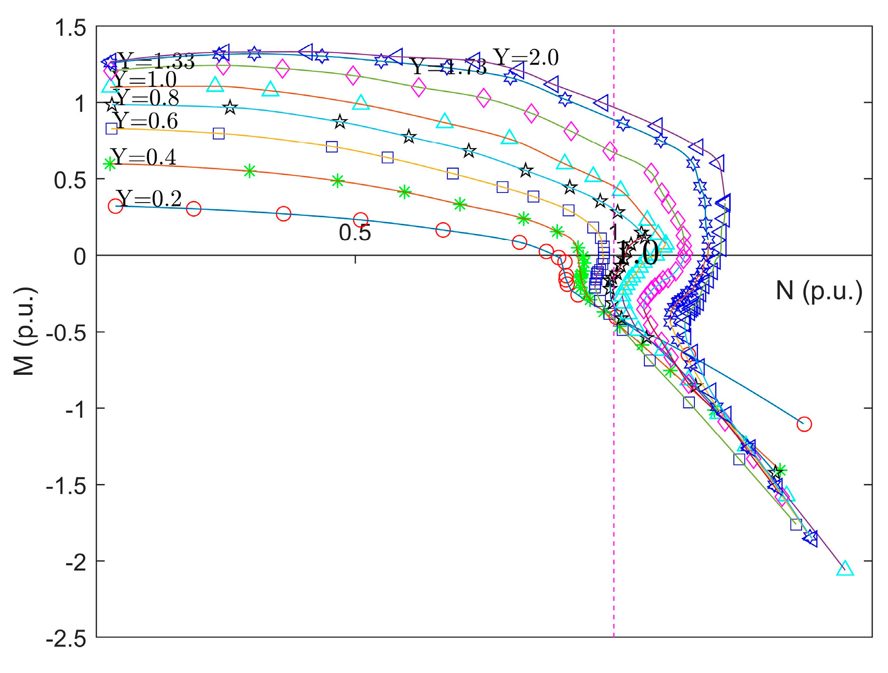
After standardizing the experimental data, the complete characteristic curve of the pump-turbine in the generating mode can be drawn, as shown in Figure 2 and Figure 3. As shown in the figures, N represents the pump-turbine speed, M represents the pump-turbine torque, and Y represents the guide vane opening. As shown in Figure 2, along the constant guide vane opening line, with the increase of the unit speed, the centrifugal braking function increases rapidly, which makes the flow and torque in the turbine direction decrease rapidly.

3.2.2. Acquisition of Transfer Coefficients

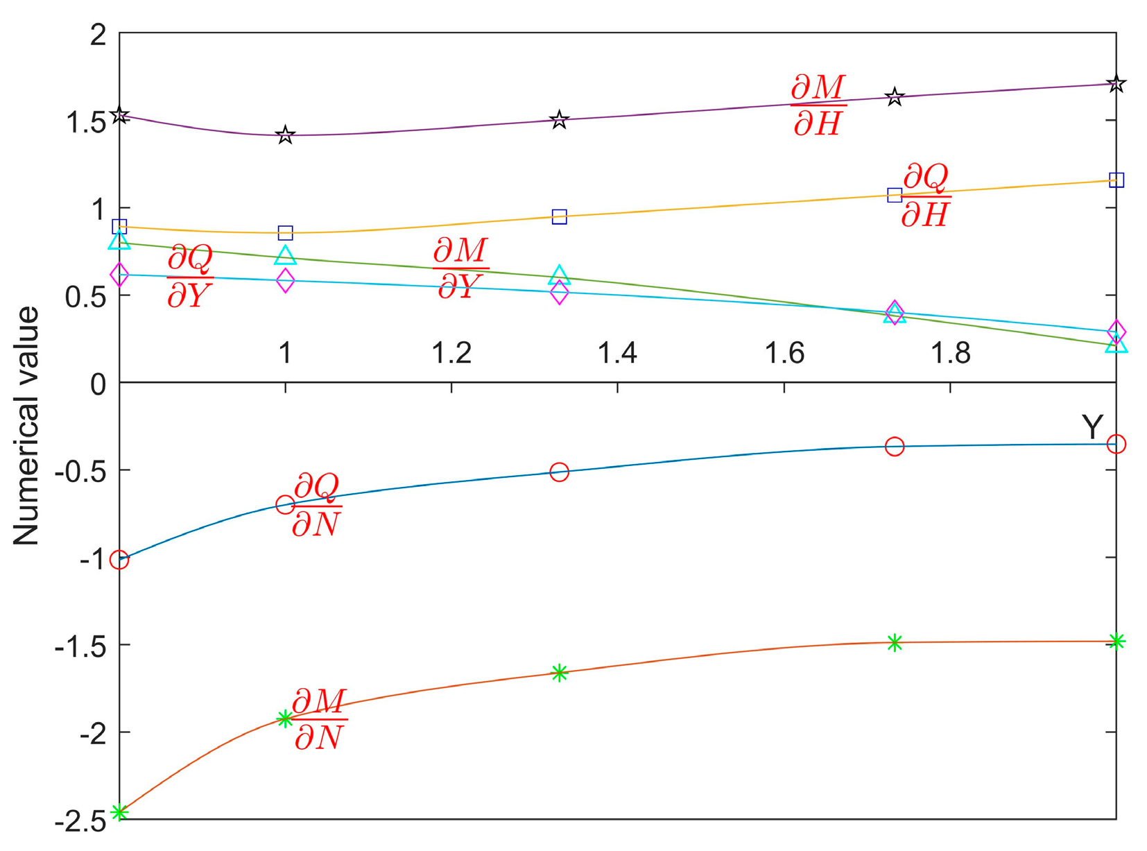
It is known that the tangent slope at different points of the complete characteristic curve is the value of the corresponding transfer coefficient. According to the complete characteristic curve in Figure 3, ex represents the derivative of the torque-speed relationship curve of the pump-turbine when the opening and the head of the operating guide vane are constant. The opening of the guide vane is always constant, and by taking multiple operating points on the equal opening line, the tangent slopes of multiple operating points in different opening lines can be obtained, and then the transfer coefficients of the torque with respect to the speed can be drawn according to these points. The change curve is shown in Figure 4. The remaining coefficients ey, eqx, and eqy can be calculated and obtained by using the same method in the torque diagram or flow diagram. In the approximate calculation, the nearby points can be selected for the difference equations, so as to obtain the tangent slope of the working point. The transfer coefficients eh and eqh of the torque and flow with respect to the head can be derived from other known coefficients according to the Formulas (21) and (22) of these two transfer coefficients [44,45]:
M H = M H N 2 H M N ,
Q H = Q 2 H N 2 H Q N ,
Through the above solving process, according to Figure 4, the transfer coefficients in front of the first partial derivative of the pump-turbine mathematical model can be obtained, and the transfer coefficients are applied to the Models (18)–(20) for load disturbance simulation test and dynamic analysis of the system.

4. Nonlinear Dynamics Analysis of the System

4.1. Nonlinear Dynamics Analysis of the System under Load Rejection Conditions

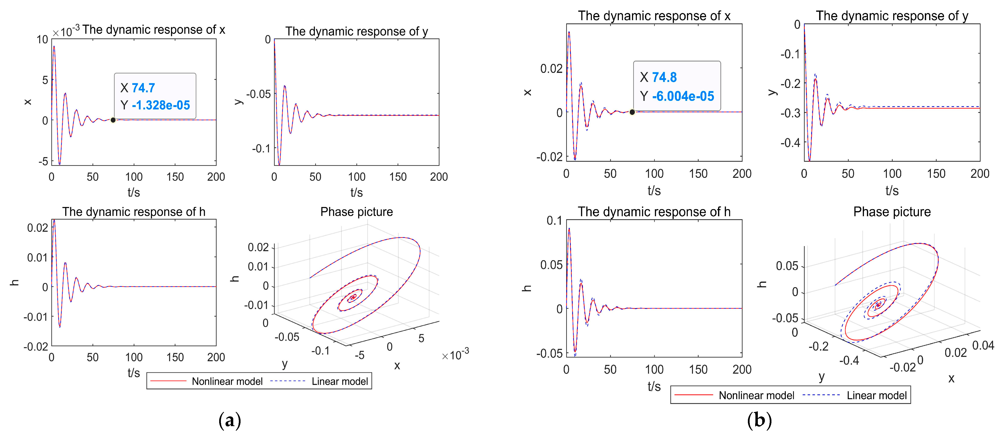
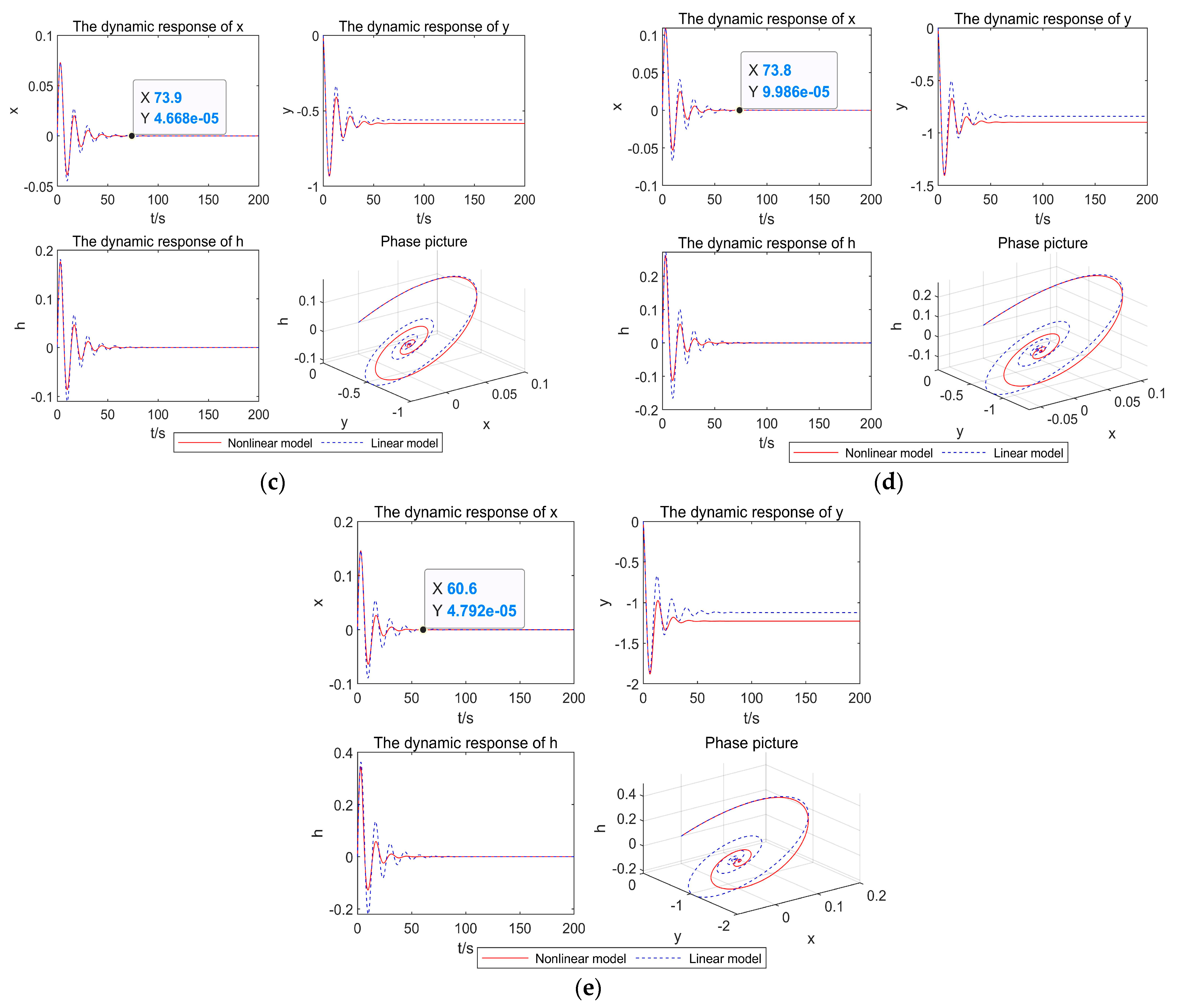
The system parameters are set to Ta = 8.86 s, Tw0 = 1.5 s, eg = 1.5, Kp = 2.0, Ki = 2.95, and the six transfer coefficients can be obtained from Figure 4, which are ex = −1.925, ey = 0.7133, eh = 1.413, eqx = −0.7, eqy = 0.5833, and eqh = 0.8555. In the transient process of load rejection fluctuation, dynamic analysis is performed on the space state equation under the working conditions of 5, 20, 40, 60, and 80% of load rejection, respectively, and the values of the coefficient mg are set to the values of −0.05, −0.2, −0.4, −0.6, and −0.8, respectively.
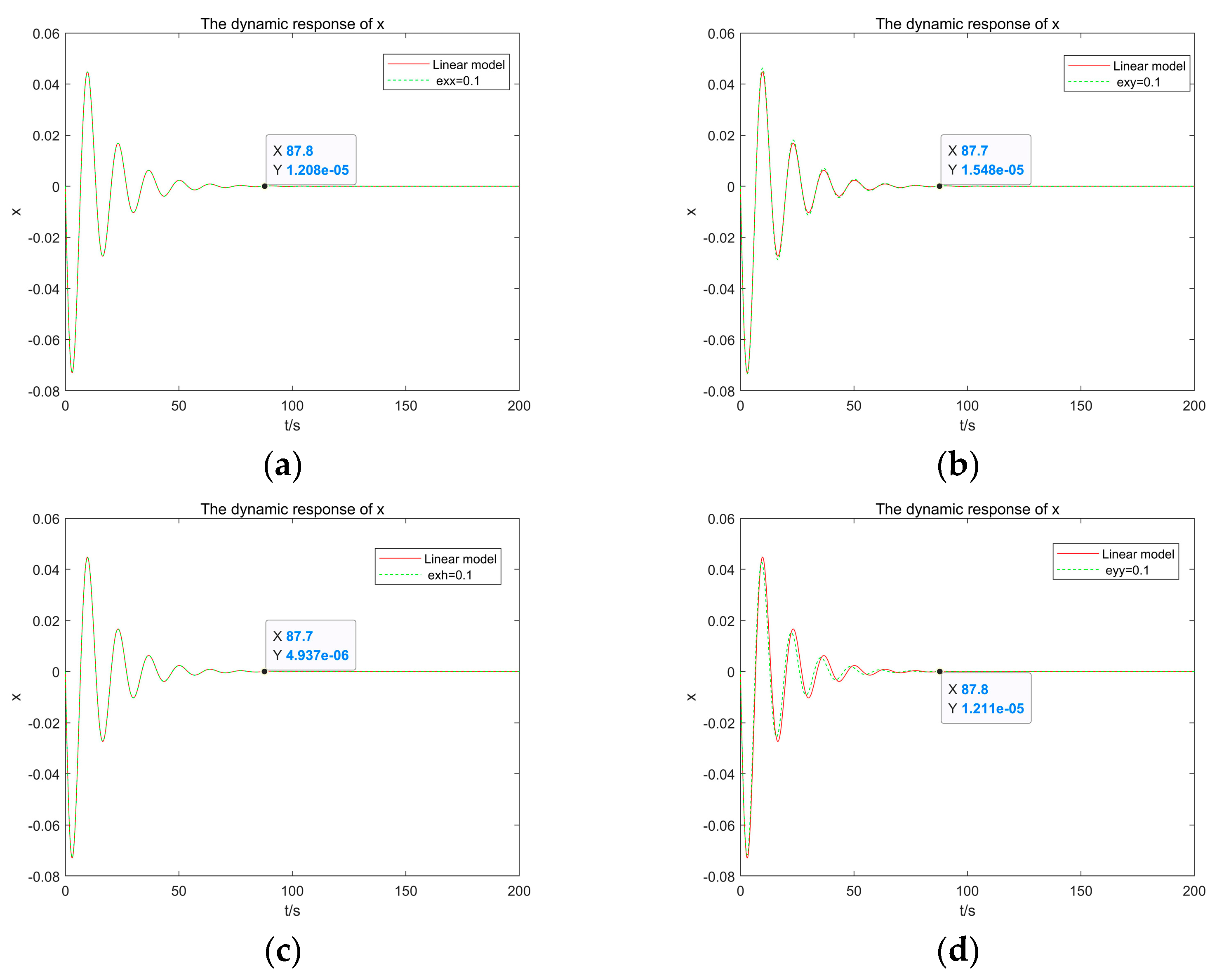
The coefficients of Taylor’s second derivative term in the space state are where Equations (18)–(20) are assigned. When the coefficients of Taylor’s second derivative term are all zero, the linear model of the system at this operating point can be obtained. Additionally, when the coefficients of Taylor’s second derivative term are not all zero, the nonlinear model of the system at this operating point can be obtained. Before the simulation, we perform a trial calculation on the coefficients of Taylor’s second-order derivative term, as shown in Figure 5. According to the simulation results, the smaller the coefficients of second derivative term, the closer the simulation results of the nonlinear model are to those of the linear model. When the coefficient of the second derivative term is larger, the difference between the simulation results of the nonlinear model and the linear model is larger. As the values of the second derivative terms are not completely known, in order not to amplify the influence of the second derivative terms on the simulation results of the nonlinear model, but also to form a certain contrast with the results of the linear model, we choose a conservative value of 0.1 for the coefficients of the second derivative term.
In this simulation, the coefficients of Taylor’s second derivative term of the nonlinear model are all set to 0.1, and the dynamic responses of each state variable in the linear model and the nonlinear model are obtained, respectively, and the phase trajectory diagram of the system can be drawn according to the dynamic response process of each variable. Taking x, y, h as the state variables, the dynamic response and the phase space trajectory of the three state variables; x, y, h of the linear model and second-order nonlinear model are drawn, respectively.
According to the above simulation results, we can get the approximate time for the system to reach the equilibrium point in the process of load rejection, which is listed in Table 2.
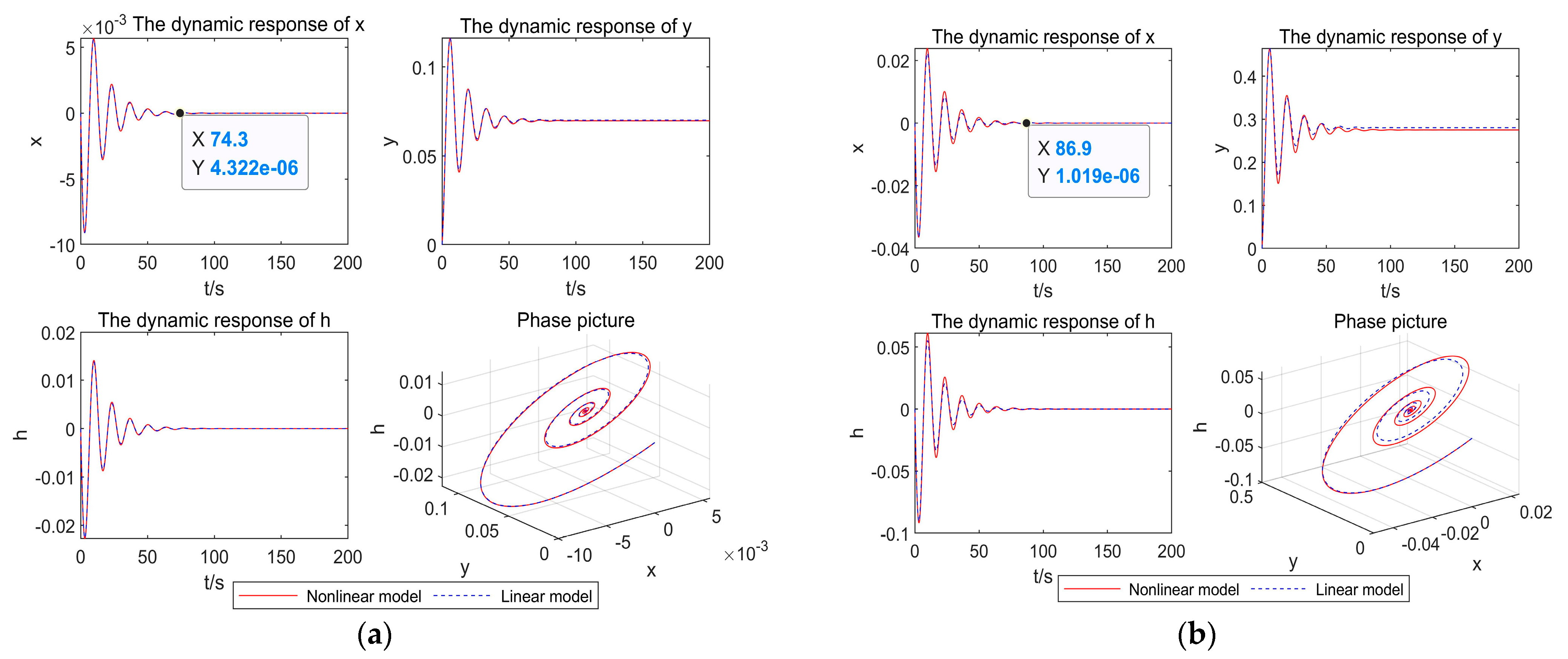
The results show that under load rejection conditions, the pump-turbine can resist external load interference through the speed control system to make the unit operate safely and stably. It can be seen from Figure 6 that the relative deviation value of the pump-turbine speed, the relative deviation value of the unit head, and the relative deviation value of the guide vane opening dynamically respond for the linear model and the nonlinear model, and they are all expressed as: the periodic damping oscillation occurs and this oscillation finally approaches to zero, the corresponding phase trajectories also show a trend of convergence, and finally, stabilize at the equilibrium point.
The specific situation is as follows: in the initial stage of load rejection, the load disturbance is extremely small. From the dynamic response diagram of 5% load rejection, it can be seen that the system can resist the external disturbance and finally make each state variable stable at the equilibrium point. When the disturbance is extremely small, the dynamic responses of each state variable in the linear model and the nonlinear model are approximately the same, and the time for each state variable to reach the equilibrium point is substantially the same after the adjustment by the regulating system.
As the disturbance of external load gradually increases, when the load rejection is 20%, the amplitude of each state variable in the linear model and the nonlinear model shows a continuous decay, and substantially decays to the equilibrium point at the same time, and the amplitude is substantially equal. However, with the continuous increase of load shedding disturbance, the gap between the dynamic responses corresponding to the linear model and the nonlinear model gradually becomes larger. The dynamic response of each state variable in the nonlinear model is more attenuated than that in the linear model. Besides, the time for each state variable to decay to the equilibrium point is shorter in the nonlinear model, so the corresponding phase trajectory diagram can converge to the equilibrium point more quickly.

4.2. Nonlinear Dynamics Analysis of the System under Load Increasing Conditions

The same system parameters are set as in the load rejection condition. In the process of load increase, the dynamic analysis of the space state equation is carried out at the operating points with load increase of 5, 20, 40, 60, and 80% respectively, and the corresponding mg are set to the values of 0.05, 0.2, 0.4, 0.6, and 0.8, respectively.
According to the above simulation results, we can get the approximate time for the system to reach the equilibrium point in the process of load increasing, which is listed in Table 3.
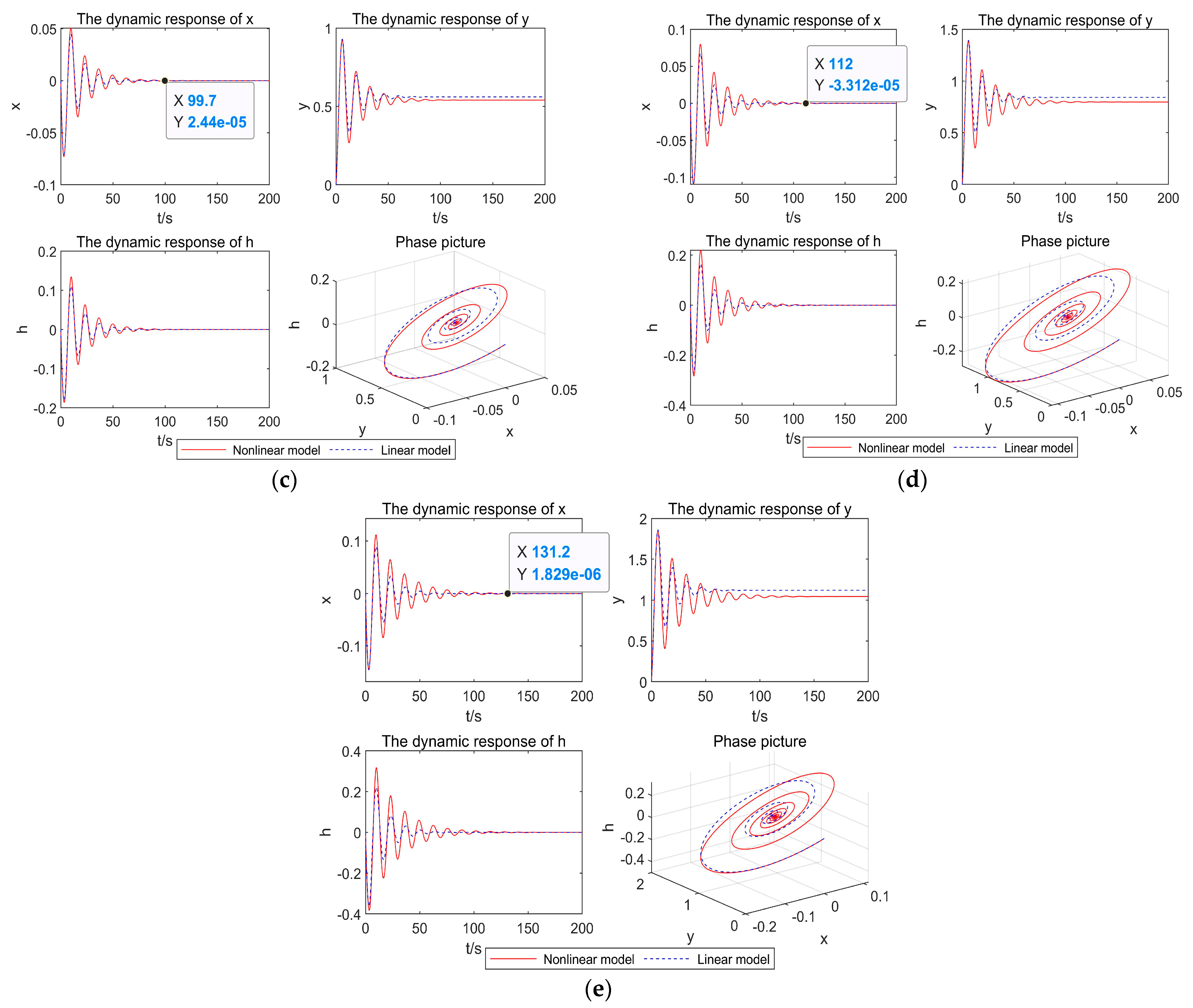
It can be seen from Figure 7 that the dynamic responses of each state variable in the linear model and the nonlinear model is as follows: the periodic damping oscillation occurs and this oscillation eventually approaches to zero, and the trajectory graph also shows a trend of convergence, and finally stabilizes at the equilibrium point. The above dynamic characteristics show that the pump-turbine can resist external load interference through the speed control system to make the unit operate safely and stably.
When the load is increased by 5%, the regulating system can quickly adjust the state variables to stabilize the state variables at the equilibrium point. When the load disturbance is small, the dynamic response diagrams for the linear model and the nonlinear model are roughly the same, and the time for each state variable to reach the equilibrium point after the system adjustment is also roughly the same.
As the disturbance of external load gradually increases, when the load is increased by 20%, the amplitudes of the state variables in the linear model and the nonlinear model both show continuous decay, and substantially decay to the equilibrium point at the same time, and the amplitudes are substantially the same. However, with the increase of load disturbance, the dynamic response for the linear model does not change much. The state variables in the nonlinear model oscillate more violently than those in the linear model, and the time for each state variable to decay to the equilibrium point increases with the increase of load disturbance.

4.3. Sensitivity Analysis of Second Derivative Terms

According to the dynamic response results of the pump-turbine governing system, we can find that there are some differences between the nonlinear model and the linear model. In order to better understand the influence of the design characteristics of pump-turbine on the system operation results, we analyzed the nonlinear second derivative terms.
In order to facilitate our observation, we choose the operating point where the dynamic response results of linear model and nonlinear model are quite different for analysis, and analyze the nonlinear model when the load is increased by 40%. The method we adopt is to set the coefficients of the second derivative term of the nonlinear model to simulate the system if and only if it is not zero, and compare the simulation results with those of the linear model to find the second derivative term that has influence on the nonlinear model in turn. In this simulation, we still use the previous parameter values for simulation.
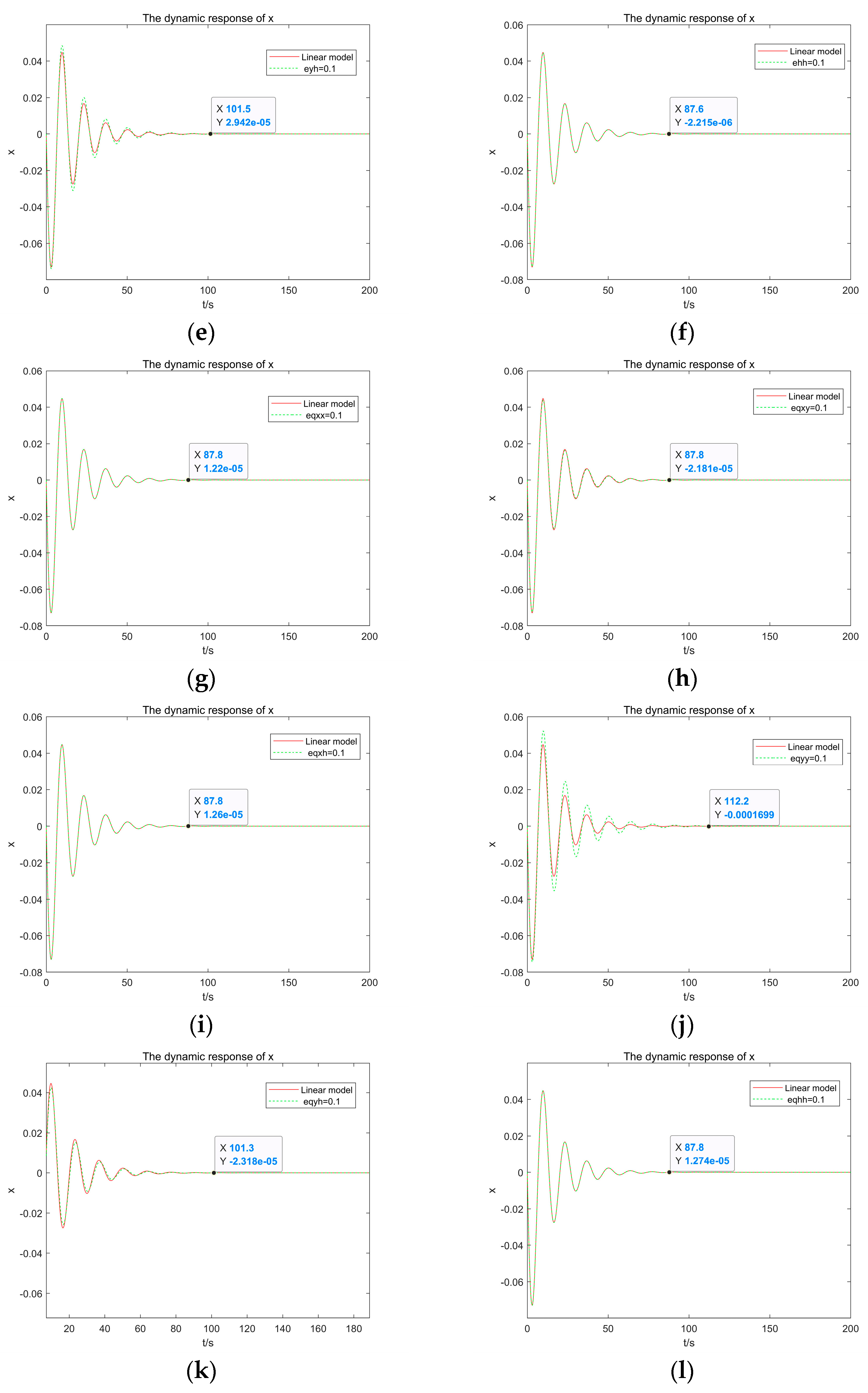
According to the simulation results in Figure 8, we found that when the coefficients eyh, eqyy, and eqyh are not zero, there is a gap between the linear model and the nonlinear model. When the other coefficients are not zero, there is a difference between the linear model and the nonlinear model. The influence of the model is very small and can be ignored. According to the simulation results in the previous chapter, the linear model roughly reaches the equilibrium state at t = 87.8 s. When the coefficient eyh is not zero, the nonlinear system roughly reaches the equilibrium point at t = 101.5 s, and the amplitude is larger than that of the linear model time domain diagram. Therefore, the product of the corresponding second derivative term yh has a significant impact on the nonlinear system. When the coefficient eqyy is not zero, the nonlinear system roughly reaches the equilibrium point at t = 112.1 s, and the graph oscillates more severely than the linear model time domain diagram, so the corresponding second derivative term y2 has an impact on the non-system which is more significant. When the coefficient eqyh is not zero, the nonlinear system roughly reaches the equilibrium point at t = 101.3 s, and the graph oscillation is gentler than that of the linear model time domain graph. However, when the linear model variables tend to stabilize in the later stage, the nonlinear model has been in a small oscillation state at this time, so the corresponding second derivative term y2 has a certain impact on the non-system.
According to the results of this system simulation, we can get that the second derivative terms yh and y2 have a certain influence on the nonlinear model, and they cannot be ignored.

5. Discussion

The nonlinear model for the pump-turbine is established by retaining Taylor’s second-order nonlinear terms of hydraulic turbine flow equation and torque equation. Then, a regulating system model containing the nonlinear pump-turbine model is established and simulated. When the load disturbance is reduced, there is little difference between the oscillation amplitude of each state variable in the linear model and the nonlinear model when load disturbance is small, and the time to reach the equilibrium point is roughly the same. However, with the increase of load disturbance, the nonlinear model can reach the equilibrium state more quickly, that is, the nonlinear model can reveal the equilibrium time of the system more accurately when the load reduction disturbance is greater, thus reducing the unnecessary adjustment time in the linear model and highlighting the adjustment quality by the regulating system.
When the load disturbance is increased and the load disturbance is small in the initial stage, the dynamic responses of each state variable in the linear model and the nonlinear model is approximately the same, the time for each state variable to reach the equilibrium point is approximately the same, and the attenuation degree of each state variable is substantially the same. With the increase of load disturbance, the state variables in the nonlinear model oscillate more violently, and the time for each state variable to reach the equilibrium point increases. Therefore, compared with the linear model, the nonlinear model can more accurately reveal the change process of unit speed, guide vane opening and water head when the load is increased. Therefore, it is possible to avoid the operation of the unit during the adjustment of the speed control system which is ignored by the linear model, so that the unit can operate more safely and stably.
After analyzing the second-order derivative terms, the second-order derivative terms yh and y2 that have a major influence on the results are found, which will also help to understand the design characteristics of the reversible pump-turbine more deeply.
Therefore, compared with the linear model, the establishment of the nonlinear model for the pump-turbine can reveal the dynamic response of the unit more effectively and accurately, improve the understanding of the system regulation process, enable a better grasp of the regulation quality of the speed control system and a deeper understanding of the operation state of the unit, thus meeting the requirements of high-precision simulation, and safe and stable operation of the unit. The establishment of the nonlinear model of the pump-turbine provides a further guarantee for the safe and stable operation of pumped storage units, promotes the development of hydropower energy development in a more efficient and mature direction, and is of great significance to the transformation of energy structure and the promotion of clean energy and renewable energy.
However, at present, the values of the second derivative coefficients of the nonlinear model are not completely known, and the nonlinear model is now in the theoretical research stage, and its application effect has not been verified in practical engineering, so it may still be reasonable to use the linear model in practical engineering. In the future research, the coefficients of second-order nonlinearity can be deduced and solved, so as to obtain a more accurate nonlinear model, which will play a vital role in the more stable and safe operation of the unit when applied to practical projects.

Author Contributions

Conceptualization, L.W. and W.Z.; methodology, L.W.; software, K.Z.; validation, L.W. and W.Z.; formal analysis, L.W. and W.Z.; resources, L.W.; writing—original draft preparation, K.Z.; writing—review and editing, L.W. and W.Z.; visualization, K.Z.; supervision, L.W.; project administration, L.W.; funding acquisition, L.W. All authors have read and agreed to the published version of the manuscript.

Funding

This work was supported in part by the National Natural Science Foundation of China (11972144 and 12072098), and the One Hundred Outstanding Innovative Scholars of Colleges and Universities in Hebei Province of China (SLRC2019022).

Institutional Review Board Statement

Not applicable.

Informed Consent Statement

Not applicable.

Data Availability Statement

Not available.

Conflicts of Interest

The authors declare no conflict of interest.

References

  1. Bitew, G.T.; Han, M.; Mekonnen, S.A.; Patrobers, S.; Khan, Z.W.; Tuan, L.K. Pumped energy storage system technology and its AC–DC interface topology, modelling and control analysis: A review. J. Eng. 2019, 2019, 705–710. [Google Scholar] [CrossRef]
  2. Xiong, Y. Analysis on Model Test of Pump Turbine for Fujian Zhouning Pumped-Storage Power Station. Hydropower Pumped Storage 2020, 6, 65–69. [Google Scholar]
  3. Cai, W.J.; Wang, Y.T.; Shi, H.D.; Zhang, M.J.; Xu, Q. Study on Optimization Strategy of Speed and Opening of Variable Speed Pumped Storage Unit. Large Electr. Mach. Hydraul. Turbine 2020, 4, 58–63. [Google Scholar]
  4. Liu, D.M.; Xu, W.L.; Zhao, Y.Z. Study on Cavitation and Operation Characteristics of Variable Speed Pumped Storage Units. Hydropower Pumped Storage 2020, 6, 36–45. [Google Scholar]
  5. Wang, L.K.; Lu, J.L.; Liao, W.L.; Zhao, Y.P.; Ji, Q.F. Numerical Analysis of the Hydraulic Force of a Pump Turbine under Partial Load Conditions in Turbine Mode; IOP Publishing: Bristol, UK, 2019; Volume 240, p. 72041. [Google Scholar]
  6. Lv, C.; Xu, Y.; Wu, X.; Zhang, Q. Characteristic Analysis and Optimal Regulation of Primary Frequency Regulation Condition in Low Water Head Area Based on Hydraulic-Mechanical-Electrical Coupling Model of Pumped Storage Unit. Complexity 2020, 2020, 6161784. [Google Scholar] [CrossRef] [Green Version]
  7. Men, C.S. Study on Dynamic Characteristics of Regulating System Based on Hydro-Turbine Compound Model Tocom-binedinternal Model and External Model. Ph.D. Thesis, Xi’an University of Technology, Xian, China, 2018. [Google Scholar]
  8. Zhao, W.; Shi, T.; Wang, L.; Cao, Q.; Zhang, H. An adaptive hybrid atom search optimization with particle swarm optimization and its application to optimal no-load PID design of hydro-turbine governor. J. Comput. Des. Eng. 2021, 8, 1204–1233. [Google Scholar] [CrossRef]
  9. Xu, Y.H. Study on Parameter Identification and Control Optimization of Governing System for Pumped Storage Unit. Ph.D. Thesis, Huazhong University of Science and Technology, Wuhan, China, 2017. [Google Scholar]
  10. Zhang, C. Study on Nonlinear Identification and Control Optimization of Pumped Turbine Governing System. Ph.D. Thesis, Huazhong University of Science and Technology, Wuhan, China, 2018. [Google Scholar]
  11. Xu, X.Y.; Guo, W.C. Stability of Speed Regulating System of Hydropower Station under Effect of Nonlinear Turbine Charac-teristics. Hydropower Energy Sci. 2020, 38, 121–125. [Google Scholar]
  12. Liu, J.Y. Characteristic Analysis of Typical Transient of Pumped Storage Power Station Based on Characteristic Curve. Master’s Thesis, Northwest Agriculture and Forestry University, Shanxi, China, 2017. [Google Scholar]
  13. Zhou, J.; Zhao, Z.; Zhang, C.; Li, C.; Xu, Y. A Real-Time Accurate Model and Its Predictive Fuzzy PID Controller for Pumped Storage Unit via Error Compensation. Energies 2017, 11, 35. [Google Scholar] [CrossRef] [Green Version]
  14. Zhang, H. Transient Dynamical Modeling and Stability Analysis of Hydroelectric Powersystems. Ph.D. Thesis, Northwest Agriculture and Forestry University, Shanxi, China, 2019. [Google Scholar]
  15. Zhao, Z.; Yang, J.; Yang, W.; Hu, J.; Chen, M. A coordinated optimization framework for flexible operation of pumped storage hydropower system: Nonlinear modeling, strategy optimization and decision making. Energy Convers. Manag. 2019, 194, 75–93. [Google Scholar] [CrossRef]
  16. Fang, Z. Research on intelligent control of hydraulic turbine governing system. Intell. City 2021, 7, 49–50. [Google Scholar]
  17. Xia, X.; Ji, J.; Li, C.-S.; Xue, X.; Wang, X.; Zhang, C. Multiobjective Optimal Control for Hydraulic Turbine Governing System Based on an Improved MOGWO Algorithm. Complexity 2019, 2019, 3745924. [Google Scholar] [CrossRef]
  18. Piraisoodi, T.; Siluvairaj, W.I.M.; Kappuva, M.A.K. Multi-objective robust fuzzy fractional order proportional–integral–derivative controller design for nonlinear hydraulic turbine governing system using evolutionary computation techniques. Expert Syst. 2019, 36, e12366. [Google Scholar] [CrossRef]
  19. Xiao, Y.; Liu, W.; Wang, G.H.; Xia, C.; Li, Z.Q.; Yu, D.H.; Ma, C.Y. Source-grid Coordination of Hydraulic Turbine Governing System. Power Syst. Technol. 2021, 45, 1852–1861. [Google Scholar]
  20. Chang, Y.; Su, H.C.; Li, X.Q.; Yang, Y.Q.; Hou, Y.Z. Analysis of Transient Stability Methods of Power System. Yunnan Electr. Power Technol. 2007, 2, 1–4. [Google Scholar]
  21. Zhang, J.L.; Ou, J.P.; Yu, D.R. Rule self-adjusting fuzzy control method based on phase plane trajectory characteris-tics. Control. Theory Appl. 2003, 4, 607–611. [Google Scholar]
  22. Zhang, H.; Su, D.; Guo, P.; Zhang, B.; Mao, Z. Stochastic dynamic modeling and simulation of a pump-turbine in load-rejection process. J. Energy Storage 2021, 35, 102196. [Google Scholar] [CrossRef]
  23. Xu, B.; Chen, D.; Zhang, H.; Wang, F. Modeling and stability analysis of a fractional-order Francis hydro-turbine governing system. Chaos Solitons Fractals 2015, 75, 50–61. [Google Scholar] [CrossRef]
  24. Chen, D.; Ding, C.; Do, Y.; Ma, X.; Zhao, H.; Wang, Y. Nonlinear dynamic analysis for a Francis hydro-turbine governing system and its control. J. Frankl. Inst. 2014, 351, 4596–4618. [Google Scholar] [CrossRef]
  25. Nagode, K.; Škrjanc, I. Modelling and Internal Fuzzy Model Power Control of a Francis Water Turbine. Energies 2014, 7, 874–889. [Google Scholar] [CrossRef] [Green Version]
  26. Liang, J.; Yuan, X.; Yuan, Y.; Chen, Z.; Li, Y. Nonlinear dynamic analysis and robust controller design for Francis hydraulic turbine regulating system with a straight-tube surge tank. Mech. Syst. Signal Process. 2017, 85, 927–946. [Google Scholar] [CrossRef]
  27. Li, G.; Wu, X.; Cui, W.; Qiu, W.; Zhou, T. Study of Hydraulic Disturbance of Pumped Storage Unit. IOP Conf. Ser. Earth Environ. Sci. 2021, 768, 12010. [Google Scholar] [CrossRef]
  28. Zhang, H.; Chen, D.; Xu, B.; Wang, F. Nonlinear modeling and dynamic analysis of hydro-turbine governing system in the process of load rejection transient. Energy Convers. Manag. 2015, 90, 128–137. [Google Scholar] [CrossRef]
  29. Guo, W.; Yang, J.; Wang, M.; Lai, X. Nonlinear modeling and stability analysis of hydro-turbine governing system with slopin-g ceiling tailrace tunnel under load disturbance. Energy Convers. Manag. 2015, 106, 127–138. [Google Scholar] [CrossRef]
  30. Xu, Y.; Li, C.; Wang, Z.; Zhang, N.; Peng, B. Load Frequency Control of a Novel Renewable Energy Integrated Micro-Grid Containing Pumped Hydropower Energy Storage. IEEE Access 2018, 6, 29067–29077. [Google Scholar] [CrossRef]
  31. Zhang, N. Study on Nonlinear Model Parameter Identification and Control Optimization of Pumped Storage Unit Governing System. Ph.D. Thesis, Huazhong University of Science and Technology, Wuhan, China, 2019. [Google Scholar]
  32. Li, H.; Chen, D.; Zhang, H.; Wu, C.; Wang, X. Hamiltonian analysis of a hydro-energy generation system in the transient of sudden load increasing. Appl. Energy 2017, 185, 244–253. [Google Scholar] [CrossRef] [Green Version]
  33. IEEE Working Gourp. Hydraulic turbine and turbine control models for system dynamic studies. IEEE Trans. Power Syst. 1992, 7, 167–179. [Google Scholar] [CrossRef]
  34. Chen, D.; Ding, C.; Ma, X.; Yuan, P.; Ba, D. Nonlinear dynamical analysis of hydro-turbine governing system with a surge tank. Appl. Math. Model. 2013, 37, 7611–7623. [Google Scholar] [CrossRef]
  35. Wang, L.; Han, Q.; Chen, D.; Wu, C.; Wang, X. Non-linear modelling and stability analysis of the PTGS at pump mode. IET Renew. Power Gener. 2017, 11, 827–836. [Google Scholar] [CrossRef]
  36. Li, H.; Chen, D.; Zhang, H.; Wang, F.; Ba, D. Nonlinear modeling and dynamic analysis of a hydro-turbine governing system in the process of sudden load increase transient. Mech. Syst. Signal Process. 2016, 80, 414–428. [Google Scholar] [CrossRef] [Green Version]
  37. Ling, D.J.; Shen, Z.Y. Bifurcation analysis of hydro-turbine governing system with saturation nonlinearity. J. Hydro Electr. Eng. 2007, 26, 126–131. [Google Scholar]
  38. Wei, S.P. Turbine Regulation; Huazhong University of Science and Technology Press: Wuhan, China, 2009. [Google Scholar]
  39. Wu, R.Q.; Chen, J.Z. Hydraulic Transition Process of Hydropower Station; China Water Conservancy and Hydropower Press: Beijing, China, 1996. [Google Scholar]
  40. Wu, Q.Q. A Dynamic Model Establishment and Numerical Simulation of Hydraulic-Mechanical-Electric-Structural System for Hydropower Station. Ph.D. Thesis, Dalian University of Technology, Dalian, China, 2017. [Google Scholar]
  41. Zhou, X.J.; Ni, J.B.; Han, W.F.; Yang, J.; Ding, J.H. Influence of pump-turbine complete characteristic curve on transient process trajectory. Water Resour. Hydropower Eng. 2021, 52, 85–93. [Google Scholar]
  42. Chen, Y.; Wang, Y.; Dai, L.Q. Numerical treatment of synthetic characteristic curves in turbine modeling. J. Water Resour. Water Eng. 2020, 31, 155–161. [Google Scholar]
  43. Zheng, Y.; Chen, Q.; Liu, W.; Yan, D. A predictive governing control method of the pumped-storage unit based on lumped-parameter model equivalence. IOP Conf. Series Earth Environ. Sci. 2021, 774, 012141. [Google Scholar] [CrossRef]
  44. Zheng, Y.; Zhang, J. Transition Process of Hydraulic Units; Peking University Press: Beijing, China, 2008. [Google Scholar]
  45. Izena, A.; Kihara, H.; Shimojo, T.; Hirayama, K.; Furukawa, N.; Kageyama, T.; Goto, T.; Okamura, C. Practical hydraulic turbine model. In Proceedings of the 2006 IEEE Power Engineering Society General Meeting, Quebec, QC, Canada, 18–22 June 2006; p. 7. [Google Scholar]
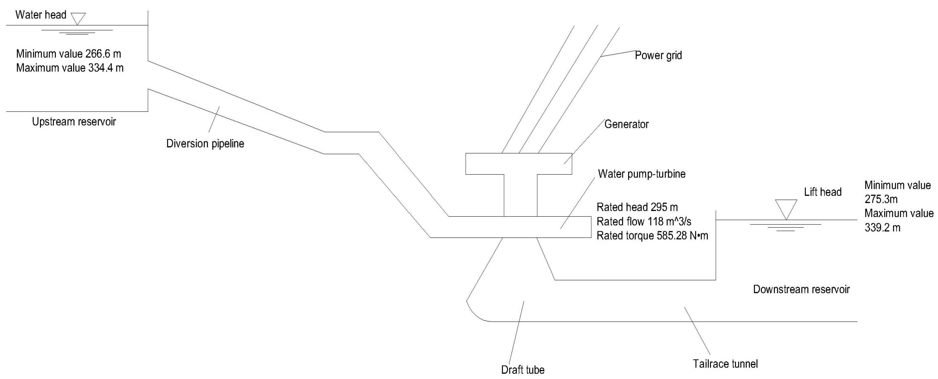
Figure 1. Schematic diagram of pumped storage power station structure.
Energies 15 00297 g001
Figure 2. N–Q standard characteristic curve of pump–turbine.
Energies 15 00297 g002
Figure 3. N–M standard characteristic curve of pump–turbine.
Energies 15 00297 g003
Figure 4. The transform curves of the transfer coefficients with respect to the guide vane opening Y ( N = 1 , H = 1 ).
Energies 15 00297 g004
Figure 5. Phase diagram of system with different coefficients.
Energies 15 00297 g005
Figure 6. Dynamic response of linear and nonlinear models with load rejection: (a) 5%; (b) 20%; (c) 40%; (d) 60%; (e) 80%.
Energies 15 00297 g006aEnergies 15 00297 g006b
Figure 7. Dynamic response of linear and nonlinear models with load increasing: (a) 5%; (b) 20%; (c) 40%; (d) 60%; (e) 80%.
Energies 15 00297 g007aEnergies 15 00297 g007b
Figure 8. Time domain plot of a nonlinear model with different second derivative terms: (a) e x x = 0.1 ; (b) e x y = 0.1 ; (c) e x h = 0.1 ; (d) e y y = 0.1 ; (e) e y h = 0.1 ; (f) e h h = 0.1 ; (g) e q x x = 0.1 ; (h) e q x y = 0.1 ; (i) e q x h = 0.1 ; (j) e q y y = 0.1 ; (k) e q y h = 0.1 ; (l) e q hh = 0.1 .
Energies 15 00297 g008aEnergies 15 00297 g008b
Table 1. Main parameters of water pump-turbine.
ParameterValue
CategoryMaximum valueMinimum value
Water head334.4 m266.6 m
Lift head 339.2 m275.3 m
Rated head295 m
Rated flow118 m3·s−1
Rated torque585.28 N·m
Table 2. Time for the system to reach the equilibrium point in the process of load rejection.
Operating PointTime/s
CategoryLinear modelNonlinear model
5%74.874.7
20%75.174.8
40%74.573.9
60%74.473.8
80%73.960.6
Table 3. Time for the system to reach the equilibrium point in the process of load increasing.
Operating PointTime/s
CategoryLinear ModelNonlinear Model
5%67.474.3
20%76.986.9
40%87.899.7
60%80.8112
80%67.4131.2
Publisher’s Note: MDPI stays neutral with regard to jurisdictional claims in published maps and institutional affiliations.