Modeling of Internal Combustion Engine Ignition Systems with a Circuit Containing Fractional-Order Elements ^†

Abstract

This paper discusses the research and analysis of the dynamics of high-voltage generating systems. The test subject is an ignition system modelled by a set of two induction coils with an open ferromagnetic core that constitutes an ignition coil. The essence of the tests involved the application of magnetic coupling of the fractional order that enabled taking into account the non-idealities of the coils and the connector that implements the ignition point. The paper contains the results of a theoretical analysis, supported by digital simulations. The conducted experiments confirm the purposefulness of the conducted analyses and the possibility of modeling real objects based on circuits with fractional-order elements.

1. Introduction

The environmental requirements imposed on modern vehicles led to a gradual withdrawal from the use of diesel engines in motor vehicles in favor of spark-ignition gasoline engines. In addition to purely electric propulsion, hybrid propulsion has become the answer to these requirements. A system composed of a gasoline engine and an electrical motor that is tasked to support the internal combustion engine at the most difficult times—when starting and during acceleration [1,2,3]—brings concrete savings in the operation of the vehicle. Hybrid cars have become an increasingly popular solution for drivers who value the environment. The two sources of propulsion work in synergy, complementing each other and providing better dynamics, greater economy, and much fewer toxic compounds released into the atmosphere.

The proper functioning of the ignition system in the operation of an internal combustion engine has a significant impact on the operation of a motor vehicle and thus has a significant impact on the environment. Its task is to provide an electric spark of the right amount of energy and at the right time, which is necessary for the ignition of the fuel–air mixture in the cylinder of the internal combustion engine [4,5,6]. Therefore, an analysis of the internal combustion engine operation and especially of its ignition system is very desirable, as it has a significant impact on the combustion process and consequently the power, torque, fuel consumption, and toxicity of exhaust gases. The ignition systems of modern vehicles are modeled with electrical circuits, the mathematical description of which in the general case is represented by a system of nonlinear equations [7,8,9].

Research on the dynamics of ignition systems is difficult and the results of analysis and digital simulations differ from experimental results. As the classical (standard) approach to the analysis of electrical systems and their modeling usually ignores the effects of non-ideality of the components, it does not always allow for the obtainment of accurate mathematical models. This is exactly the case with ignition system models.

The application of fractional order calculus to electrical circuits has opened up a new area of application that provides the possibility to approximate real elements to a degree that was not possible with the classical (integer order) approach. There are many interrelated electrical and magnetic phenomena in ignition systems in which differential calculus can be applied. These include losses in individual elements, relaxation of dielectric materials, electrochemical processes, magnetic non-homogeneity, nonlinearity, and simply operating conditions, such as temperature. For many years, there has been a significant increase in the number of research on the practical application of fractional order calculus. A review of the practical applications of this calculus is given, among others, in works on the study of electrotechnical components and devices, such as supercapacitors, resistors with memory referred to as “memristors” [10,11], as well as coils with inductance with a skin effect [12], and fractional mutual inductance coils [13,14]. Fractional order elements C_α and L described by fractional-order differentials and integral calculus are introduced as a generalization of classical elements [15,16,17,18,19].

It appears that mathematical models of a fractional order of dynamic systems are better able to describe the phenomena (processes) occurring in real objects. This is also true for electrical circuits, such as ignition systems, where hypothetical quasi-capacitive and quasi-inductive components are assumed to exist and the relationships between currents and voltages or voltages and currents are defined by a fractional-order derivative [20]:

$$i_C=C_{\alpha }\frac{d^{\alpha }{u}_C}{d{t}^{\alpha }}; u_L=L_{\alpha }\frac{d^{\alpha }{i}_L}{d{t}^{\alpha }}$$

(1)

The present paper is focused on the problem of the analysis of the operation in dynamic states of systems that generate high voltages, namely ignition systems, and their mathematical description with the use of fractional order calculus [21]. The main objective is to study two induction coils that constitute an ignition coil and its properties taking into account fractional order magnetic coupling.

This paper comprises an introduction, four sections, a conclusion, and a list of references. The introduction discusses the problem in question. Section 2 gives a synthetic presentation of the mathematical apparatus used in the analysis. The definitions of selected fractional-order derivatives are presented. The chapter discusses the basic methods used to determine the Laplace transform and its inverse for fractional-order systems, as well as the methods allowing for an approximation of the s^α, a factor with a quotient of polynomials containing integral powers of s. The next section presents a mathematical model of a distributorless ignition system with elements of the fractional order under analysis. The main part of the paper is Section 4, which shows an analysis of an ignition system model with fractional-order elements. The section contains the results of the theoretical analysis supported by digital simulation results. The results warrant the conclusion that with the developed model, it is possible to model the operation of a real ignition system more realistically. Experimental studies on a real object confirming the advisability of the analyses performed are presented in Section 5. The paper ends with a summary including a presentation of the objectives of further research and with references.

2. Selected Elements of Fractional Order Calculus

This section presents the definitions of fractional-order derivatives in Caputo’s sense and the corresponding Laplace transform. It shows the approximation methods for determining the inverse Laplace transform of fractional-order systems, including the continued fraction expansion (CFE) method and the Oustaloup method.

The definition of a derivative is obtained from the definition of the Riemann-Liouville fractional integral, which is a generalization of the formula of an nth-order integral:

$$I^{n}y\left(x\right)={{\displaystyle \int }}_0^x{{\displaystyle \int }}_0^{x_{n-1}}\cdots {{\displaystyle \int }}_0^{x_1}y\left(x_0\right)d{x}_0\dots d{x}_{n-2}d{x}_{n-1}=\frac{1}{\left(n-1\right)!}{{\displaystyle \int }}_0^x\frac{1}{{(x-t)}^{1-n}}y\left(t\right)dt$$

(2)

and from another well-known formula used in classical differential calculus:

$$\frac{d^n}{d{x}^n}f\left(x\right)=I^{k-n}\frac{d^k}{d{x}^k}f\left(x\right)$$

(3)

where the f(x) function is differentiable n times in the [a, b] interval, k, n ∈ N, and k > n.

Definition 1.

A derivative of the$\alpha \left(\alpha \in R_{+}\right)$order, in Caputo’s sense, is the operator:

$${}_a{}^{C}D{}_t^{\alpha }f\left(t\right)=I^{\left(k-\alpha \right)}\frac{d^k}{d{t}^k}f\left(t\right)=\frac{1}{\Gamma \left(k-\alpha \right)}{{\displaystyle \int }}_a^t\frac{f^{\left(k\right)}\left(\tau \right)}{{(t-\tau )}^{\alpha +1-k}}d\tau ,$$

(4)

where$k-1\le \alpha \le k$.

An important feature of Caputo’s derivative is that the initial conditions include integer-order derivatives. These derivatives have a more complete physical meaning than fractional-order derivatives; therefore, Definition (1) is of practical importance.

The Laplace transform method is a very commonly used tool for solving differential equations. The relationships on the basis of which the Laplace transform of fractional-order derivatives is determined can be calculated using the relationship for the transform of the classical nth-order derivative:

$$L\left\{f^n\left(t\right); s\right\}=s^{n}F\left(s\right)-{{\displaystyle \sum }}_{k=0}^{n-1}{s}^{n-k-1}{f}^{\left(k\right)}\left(0\right)=s^{n}F\left(s\right)-{{\displaystyle \sum }}_{k=0}^{n-1}{s}^k{f}^{\left(n+k+1\right)}\left(0\right),$$

(5)

and the convolution transform of the function:

$$L\left\{f\left(t\right)\ast g\left(t\right); s\right\}=F\left(s\right)G\left(s\right),$$

(6)

Thus, for fractional-order derivatives in the Riemann-Liouville sense:

$$L\left\{{}_0{}^{RL}D{}_x^{\alpha }f\left(t\right); s\right\}=s^{\alpha }F\left(s\right)-{{\displaystyle \sum }}_{k=0}^{n-1}{s}^k{\left[{}_0{}^{RL}D{}_x^{\alpha -k-1}f\left(t\right)\right]}_{t=0}, n-1\le \alpha <n.$$

(7)

The practical application of this transform is limited due to the lack of physical interpretation of the initial values of the fractional derivatives for the lower bound t = 0. By analogy, one can obtain a formula for the fractional derivative in the Caputo sense:

$$L\left\{{}_0{}^{C}D{}_x^{\alpha }f\left(t\right); s\right\}=s^{\alpha }F\left(s\right)-{{\displaystyle \sum }}_{k=0}^{n-1}{s}^{\alpha -k-1}{f}^k\left(0\right),n-1\le \alpha <n.$$

(8)

whose application in practice is much broader, since the initial conditions occurring here for t = 0 concern integer-order derivatives that have known physical interpretations.

For fractional-order derivatives, the Laplace transform, assuming zero initial conditions, is equal to:

$$L\left\{{}_0{}^{RL}D{}_t^{\alpha }f\left(t\right)\right\}=L\left\{{}_0{}^{C}D{}_t^{\alpha }f\left(t\right)\right\}=L\left\{{}_0{}^{GL}D{}_t^{\alpha }f\left(t\right)\right\}=s^{\alpha }F\left(s\right)$$

(9)

where F(s) is the Laplace transform of the f(t) function.

More characteristics are given in publications [22,23].

Determination of the inverse Laplace transform is done by decomposing the function into simple fractions. Therefore, the discretization of the continuous Laplace operator opens up possibilities to analyze fractional-order systems. Consequently, to achieve this, appropriate approximation techniques are required. There are a number of approximation methods used in the analysis of fractional-order systems. Examples include the following methods used for continuous time: the continued fraction expansion (CFE) method [24], Carson’s method [25], the Oustalou method [26], and the Matsuda method.

The most common methods used to determine the inverse Laplace transform of fractional-order systems are the ones that enable approximation of the s^α factor with the quotient of polynomials containing integral powers of s. One such method is the continued fraction expansion (CFE) method, which derives from an expansion into an infinite fraction of the expression (1 + x)^α,$0\le \alpha \le 1$. By substituting x = s − 1 and taking successive expressions for consideration, one obtains approximations s^α of the corresponding orders and hence of accuracy.

According to this method, the s^α factor can be represented as a quotient of polynomials of the s variable and the order of the α derivative—these variables appear here in integer powers [27,28].

$$s^{\alpha }\cong \frac{N\left(s,\alpha \right)}{D\left(s,\alpha \right)}=\frac{{{\displaystyle \sum }}_{k=0}^A{P}_{Ak}\left(\alpha \right)s^{A-k}}{{{\displaystyle \sum }}_{k=0}^A{Q}_{Ak}\left(\alpha \right)s^{A-k}}$$

(10)

where A is the order of approximation; P_Ak(α), Q_Ak(α) — α are polynomials of the A order.

As shown in publication [29], the approximation order A = 5 turns out to be the most optimal. Assuming the approximation order A = 5, these polynomials express the following form:

$$s^{\alpha }=\frac{P_{50}{s}^5+P_{51}{s}^4+P_{52}{s}^3+P_{53}{s}^2+P_{54}s+P_{55}}{Q_{50}{s}^5+Q_{51}{s}^4+Q_{52}{s}^3+Q_{53}{s}^2+Q_{54}s+Q_{55}}$$

(11)

where:

$$\begin{array}{c}{P}_{50}=Q_{55}=-a^5-15a^4-85a^3-225a^2-274a-120\hfill \\ P_{55}=Q_{50}=a^5-15a^4+85a^3-225a^2+274a-120\hfill \\ P_{51}=Q_{54}=5a^5+45a^4+5a^3-1005a^2-3250a-3000\hfill \\ P_{54}=Q_{51}=-5a^5+45a^4-5a^3-1005a^2+3250a-3000\hfill \\ P_{52}=Q_{53}=-10a^5-30a^4+410a^3+1230a^2-4000a-12000\hfill \\ P_{52}=Q_{53}=10a^5-30a^4-410a^3+1230a^2+4000a-12000\hfill \end{array}$$

It is worth noting that the polynomials present in the above approximations contain integer powers of s, so the inverse transform can be determined using the well-known methods [30,31,32,33].

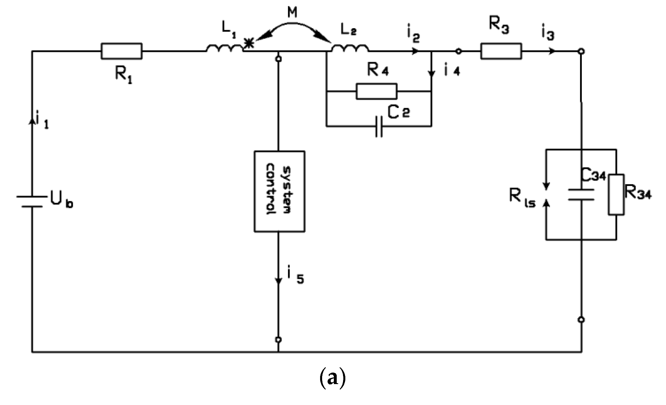
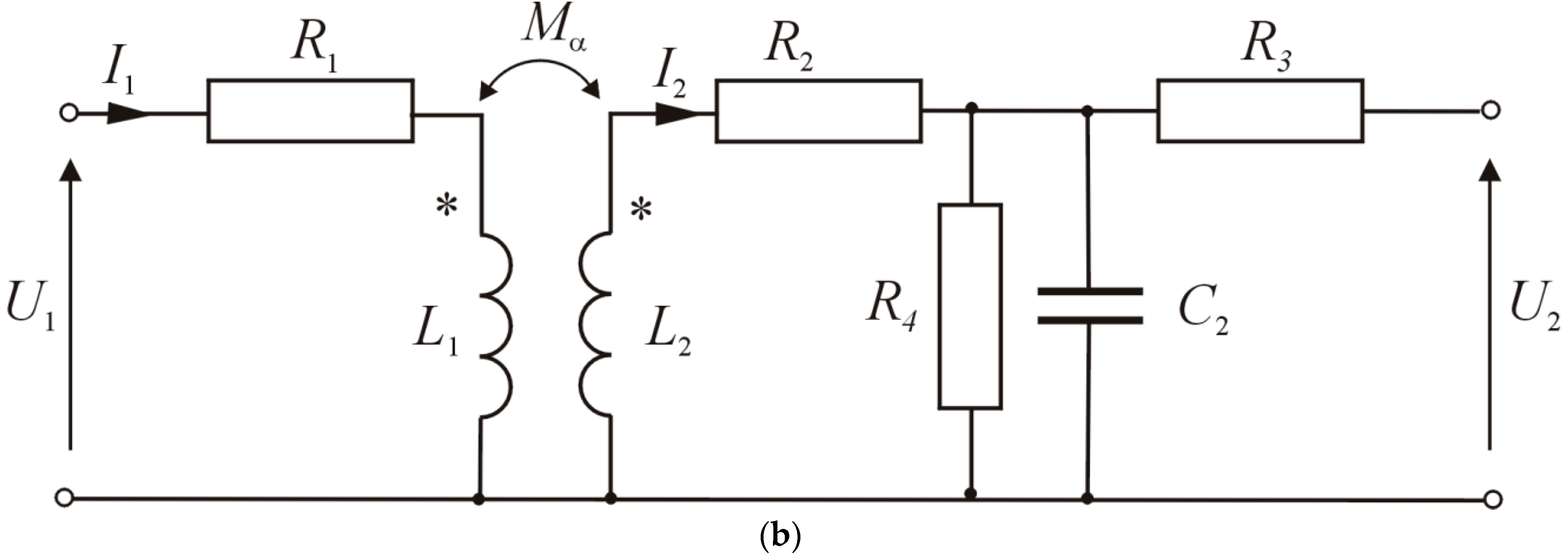
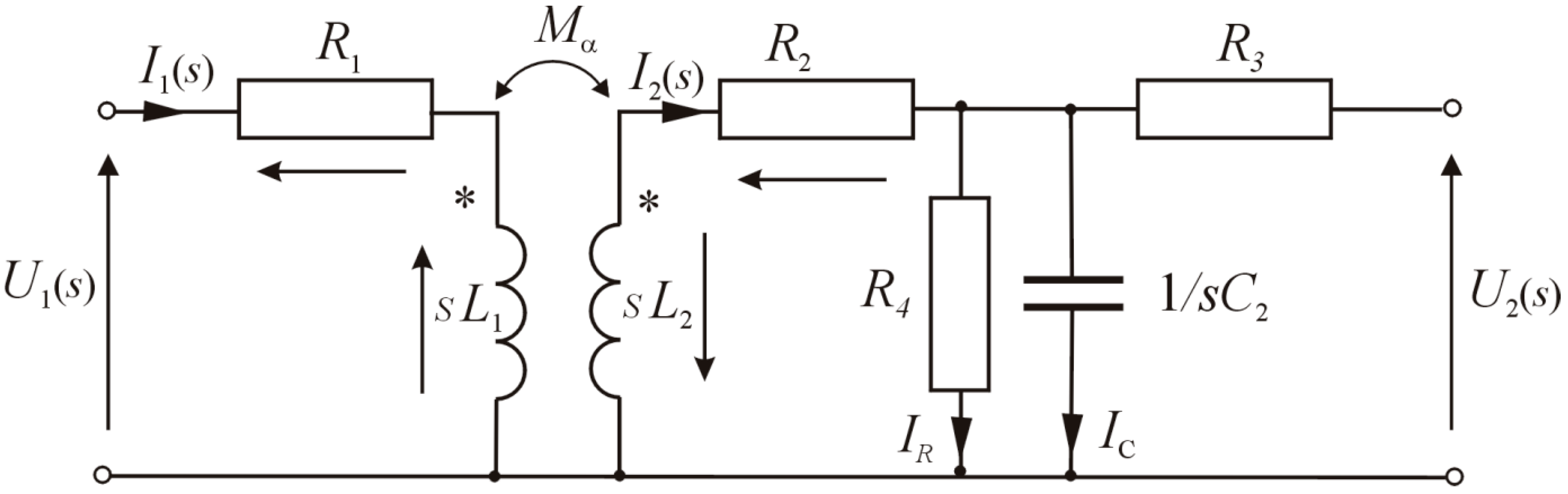
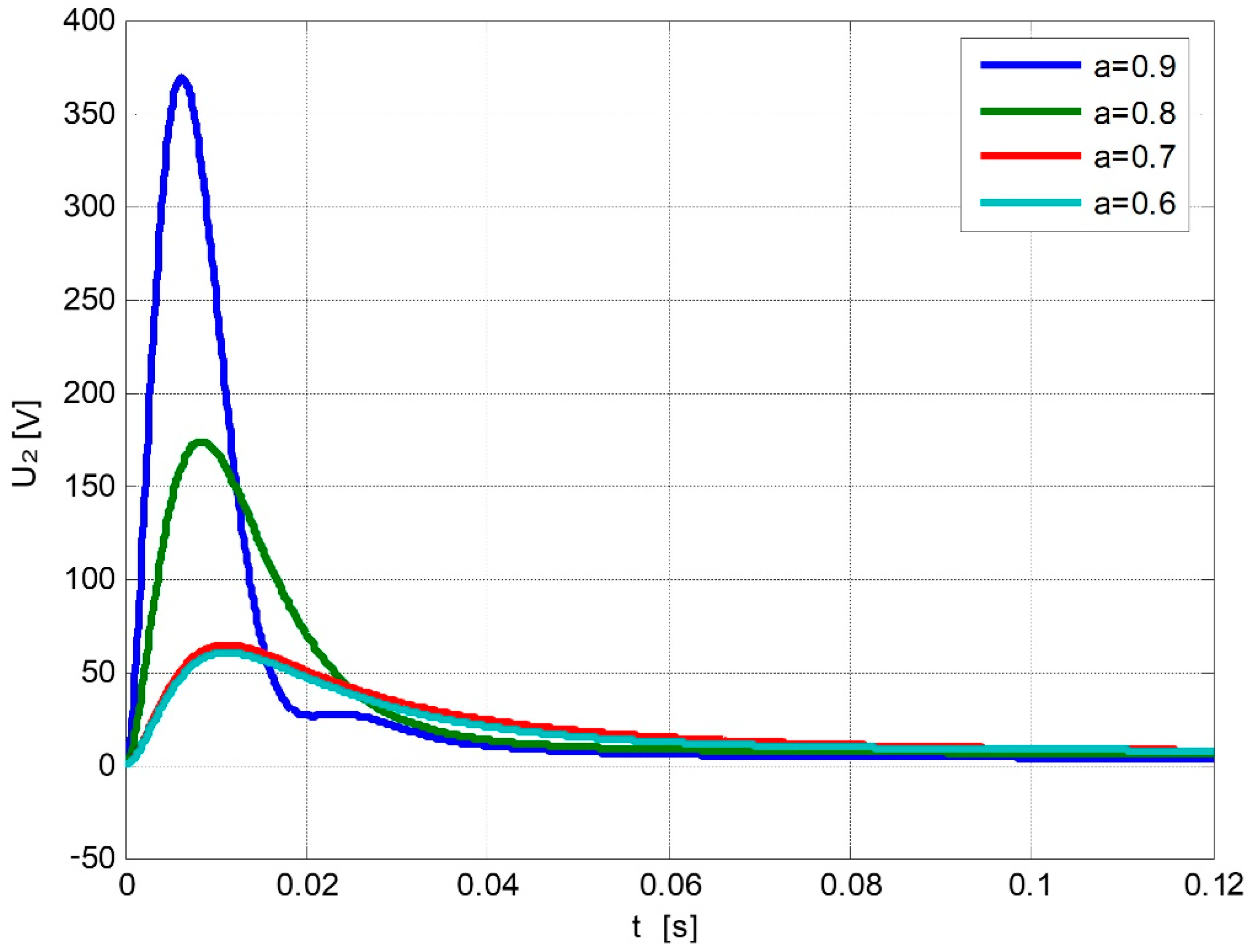
3. Distributorless Ignition System Model and Numerical Simulation Results

For the purpose of the analysis of the operation of an ignition system, a model of the ignition coil was adopted for which a fractional-order magnetic coupling was introduced between its two windings. When constructing the mathematical model of the ignition system, the following simplifying assumptions were made:

• the inductance, capacitance, and resistance of wires on the low-voltage side was omitted;
• the initial discharge voltage was assumed to be equal to the spark plug voltage; and
• the spark plug, at this stage of the analysis, was assumed to be a break in the circuit.

Considering the above assumptions, an equivalent diagram of the ignition system (Figure 1a) and an equivalent diagram of the fractional-order magnetic coupling ignition system of the ignition coil M, shown in (Figure 1b), were developed.

The following designations and values of ignition system parameters used for calculations were adopted in the analysis:

• U₁ = 13 V—battery voltage;
• R₁ = 0.9 Ω—coil primary winding resistance;
• L₁ = 0.0025 H—coil primary winding inductance;
• L₂ = 40 H—coil secondary winding inductance;
• R₂ = 6400 Ω—ignition coil secondary winding resistance;
• R₄= $\frac{1}{G_4}=$ 50 MΩ—resistance representing losses in the coil core;
• R₃ = 5 kΩ—radio interference reduction;
• C₂ = 170 pF—coil self-capacitance.

In reality, the operation of the ignition system can be divided into three stages: charging, discharging, and spark discharge represented by voltage U₂ (whose time waveform u₂(t) presents the waveform of the spark discharge voltage on the spark plug).

Currents are generally switched on or off in the primary circuit of the ignition system by mechanical–electrical or electronic switches. The electrical circuit switching is accompanied by a transient state of voltage and current, which is associated with the presence of inductance and capacitance in the circuit. Therefore, the following physical phenomena can be observed during the operation of an ignition system:

-

a current break in the ignition coil;

-

a transformation of the impulse from the primary to the secondary side (magnetic coupling);

-

conduction of a high-voltage impulse through high-voltage wires—treated as a long line;

-

an arc discharge on the spark plug.

The ignition of the fuel–air mixture in the cylinder at the right time as a result of spark discharge on the spark plug is very important from the point of view of operation of an internal combustion engine. A discharge occurs when the voltage applied to the electrodes of the spark plug ionizes the gas to the extent that an electric current can flow in the inter-electrode space and the value of the stored energy enables the initiation of this process.

A spark discharge consists of two phases:

-

a capacitive phase—a very short high-current impulse;

-

an inductive phase—a long arc discharge time (compared to the capacitive phase) with low current value.

Testing of the ignition system was carried out in two stages:

• Charging of the system—applying battery voltage to the ignition system with zero initial conditions—Figure 2a—for time $0<t<t_0$;
• Discharging the system—interruption of the power supply and opening of the primary side of the ignition coil—Figure 2b—for time $t>t_0$.

The analysis of the ignition system operation at the charging stage was carried out using the operator method based on the diagram shown in Figure 3.

For the diagram shown in Figure 3, based on Kirchhoff’s laws, it is possible (after the Laplace transform with zero initial conditions) to write a system of equations:

$$\{\begin{array}{c}{U}_1\left(s\right)=I_1\left(s\right)\left(R_1+s{L}_1\right)-s^{\alpha }{M}_{\alpha }{I}_2\left(s\right)\\ I_2\left(s\right)\left(R_2+s{L}_2\right)-s^{\alpha }{M}_{\alpha }{I}_1\left(s\right)+U_2\left(s\right)\\ I_2\left(s\right)=U_2\left(s\right)\left(G_4+s{C}_2\right)\end{array}$$

(12)

By determining U₂(s), I₁(s), and I₂(s) from that system of equations, the following equations were obtained:

$$\{\begin{array}{c}{U}_2\left(s\right)=\frac{s^{\alpha }{M}_{\alpha }{U}_1\left(s\right)}{\left(R_1+s{L}_1\right)\left(R_2+s{L}_2\right)\left(G_4+s{C}_2\right)+\left(R_1+s{L}_1\right)-s^{2\alpha }{M}_{\propto }^2\left(G_4+s{C}_2\right)}\\ I_1\left(s\right)=U_1\left(s\right)\frac{\left(R_2+s{L}_2\right)\left(G_4+s{C}_2\right)+1}{\left(R_1+s{L}_1\right)\left(R_2+s{L}_2\right)\left(G_4+s{C}_2\right)+\left(R_1+s{L}_1\right)-s^{2\alpha }{M}_{\propto }^2\left(G_4+s{C}_2\right)}\\ I_2\left(s\right)=\frac{s^{\alpha }{M}_{\alpha }\left(G_4+s{C}_2\right)U_1\left(s\right)}{\left(R_1+s{L}_1\right)\left(R_2+s{L}_2\right)\left(G_4+s{C}_2\right)+\left(R_1+s{L}_1\right)-s^{2\alpha }{M}_{\propto }^2\left(G_4+s{C}_2\right)}\end{array}$$

(13)

By replacing U₁(s) with U/s (where: U—fixed battery voltage) and replacing s^α and s^2α with the respective quotients of polynomials (determined from Equation (10)), the following equations were obtained:

$$\{\begin{array}{c}{U}_2\left(s\right)=\frac{N\left(s,\propto \right)D\left(s,2\propto -1\right)M_{\alpha }U}{Denom 1 }\\ I_1\left(s\right)=\frac{UD\left(s,2\propto -1\right)\left[\left(R_2+s{L}_2\right)\left(G_4+s{C}_2\right)+1\right]}{Denom 2 }\\ I_2\left(s\right)=\frac{UN\left(s,\propto \right)D\left(s,2\propto -1\right)M_{\propto }\left(G_4+s{C}_2\right)}{Denom 3 }\end{array}$$

(14)

in which:

$$\begin{array}{cc}\hfill Denom1& =D\left(s,\alpha \right)·\{D\left(s,2\alpha -1\right)·\left[\left(R_1+s{L}_1\right)·\left(R_2+s{L}_2\right)·\left(G_4+s{C}_2\right)+\left(R_1+s{L}_1\right)\right]\hfill \\ & -sN\left(s,2\alpha -1\right)·M_{\alpha }^2(G_4+s{C}_2\}\hfill \end{array}$$

$$\begin{array}{cc}\hfill Denom2& =D\left(s,2\alpha -1\right)·\left[\left(R_1+s{L}_1\right)·\left(R_2+s{L}_2\right)·\left(G_4+s{C}_2\right)+\left(R_1+s{L}_1\right)\right]\hfill \\ & -sN\left(s,2\alpha -1\right)·M_{\alpha }^2(G_4+s{C}_2\}\hfill \end{array}$$

$$\begin{array}{cc}\hfill Denom3& =D\left(s,\alpha \right)·\{D\left(s,2\alpha -1\right)·\left[\left(R_1+s{L}_1\right)·\left(R_2+s{L}_2\right)·\left(G_4+s{C}_2\right)+\left(R_1+s{L}_1\right)\right]\hfill \\ & -sN\left(s,2\alpha -1\right)·M_{\alpha }^2(G_4+s{C}_2\}\hfill \end{array}$$

By calculating the inverse transform for time $t>t_0$, the voltage waveforms u₂(t) at the output of the ignition system and the current waveform i₂(t) were obtained for different values of fractional α-orders of the magnetic coupling between two coils.

The voltage waveforms u₂(t) for the order α = 0.9, 0.8, 0.7, and 0.6, and the current waveforms i₂(t) for the order α = 0.9 are shown in Figure 4 and Figure 5, respectively.

The next stage of the analysis of the ignition system operation is the system discharge stage—a break in the power supply and a short circuit in the primary side of the ignition coil. At this stage, after opening of the W switch (Figure 2) after time t₀ for initial conditions i₁(t₀), i₂(t₀), and u₂₀(t₀), the following equations describing the system were obtained:

$$\{\begin{array}{c}{I}_1\left(s\right)=0 i_1\left(0\right)=i_1\left(t_0\right)\\ I_2\left(s\right)\left(R_2+s{L}_2\right)+U_{20}\left(s\right)+s^{\alpha -1}{i}_1\left(t_0\right)=0\\ I_2\left(s\right)=U_{20}\left(s\right)\left(G_4+s{C}_2\right)\end{array}$$

(15)

By determining U₂(s) and I₂(s) from that system of equations, the following was obtained:

$$\begin{array}{c}{U}_{20}\left(s\right)=\frac{-N\left(s,\alpha \right)i_1\left(t_0\right)}{sD\left(s,\alpha \right)\left[\left(G_4+s{C}_2\right)\left(R_2+s{L}_2\right)+1\right]}\\ I_2\left(s\right)=\frac{-N\left(s,\alpha \right)i_1\left(t_0\right)\left(G_4+s{C}_2\right)}{sD\left(s,\alpha \right)\left[\left(G_4+s{C}_2\right)\left(R_2+s{L}_2\right)+1\right]}\end{array}$$

(16)

The voltage waveforms u₂(t)and the current waveforms i₂(t) for the order α = 0.9 are shown in Figure 6 and Figure 7, respectively.

By combining the two stages considered, it is possible to present the complete operation cycle of the ignition system.

The results of numerical simulations that model the actual ignition system operation cycle and show the voltage waveforms u₂(t) at the output of the ignition system and the current waveforms i₂(t) for different values of the fractional orders α of the magnetic coupling between the two windings of the ignition coil are shown in Figure 8 and Figure 9.

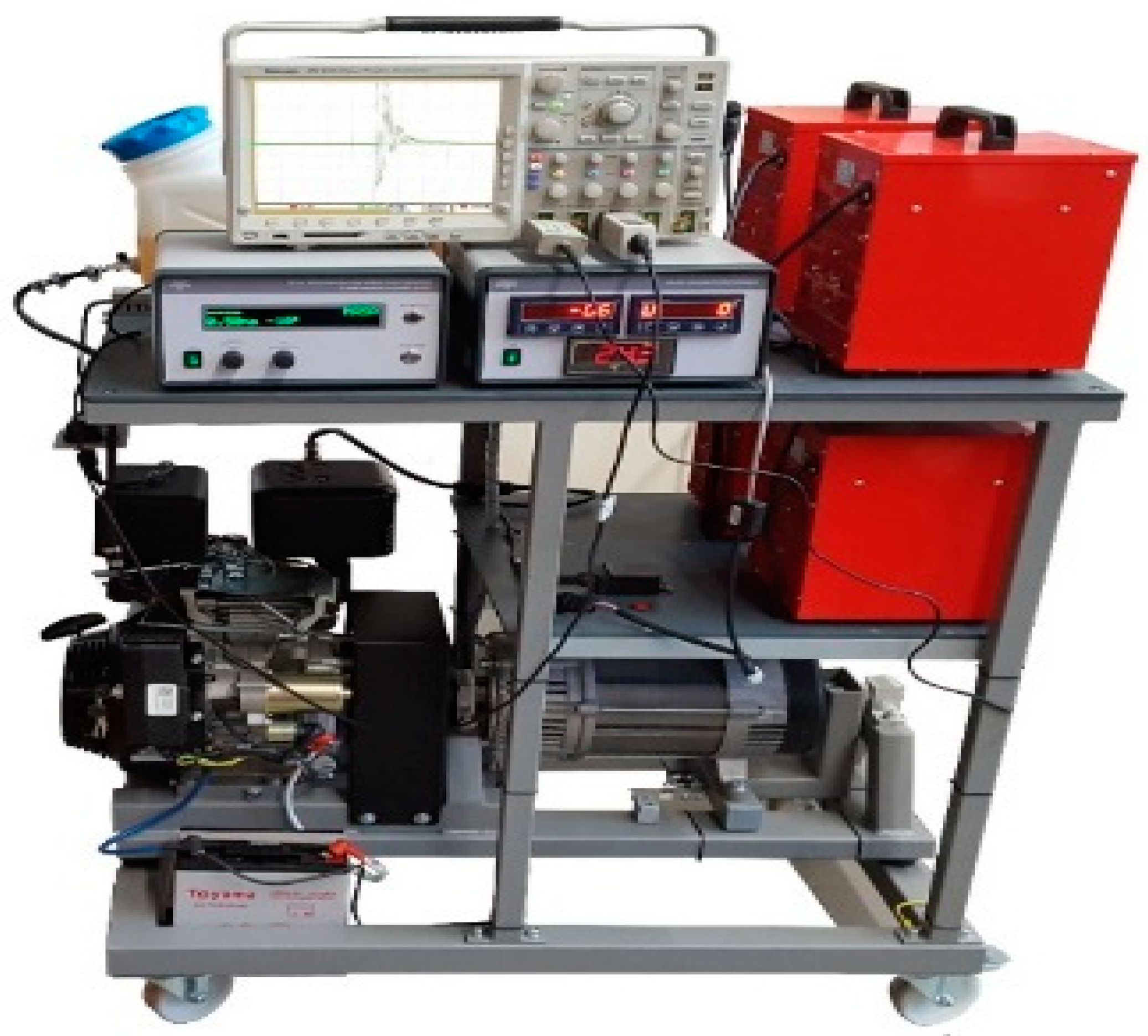
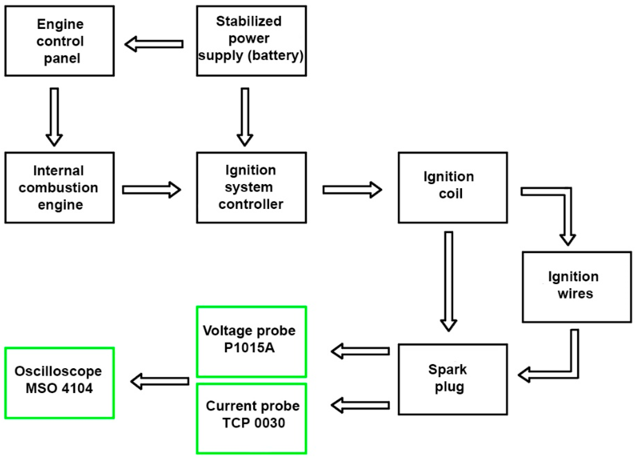
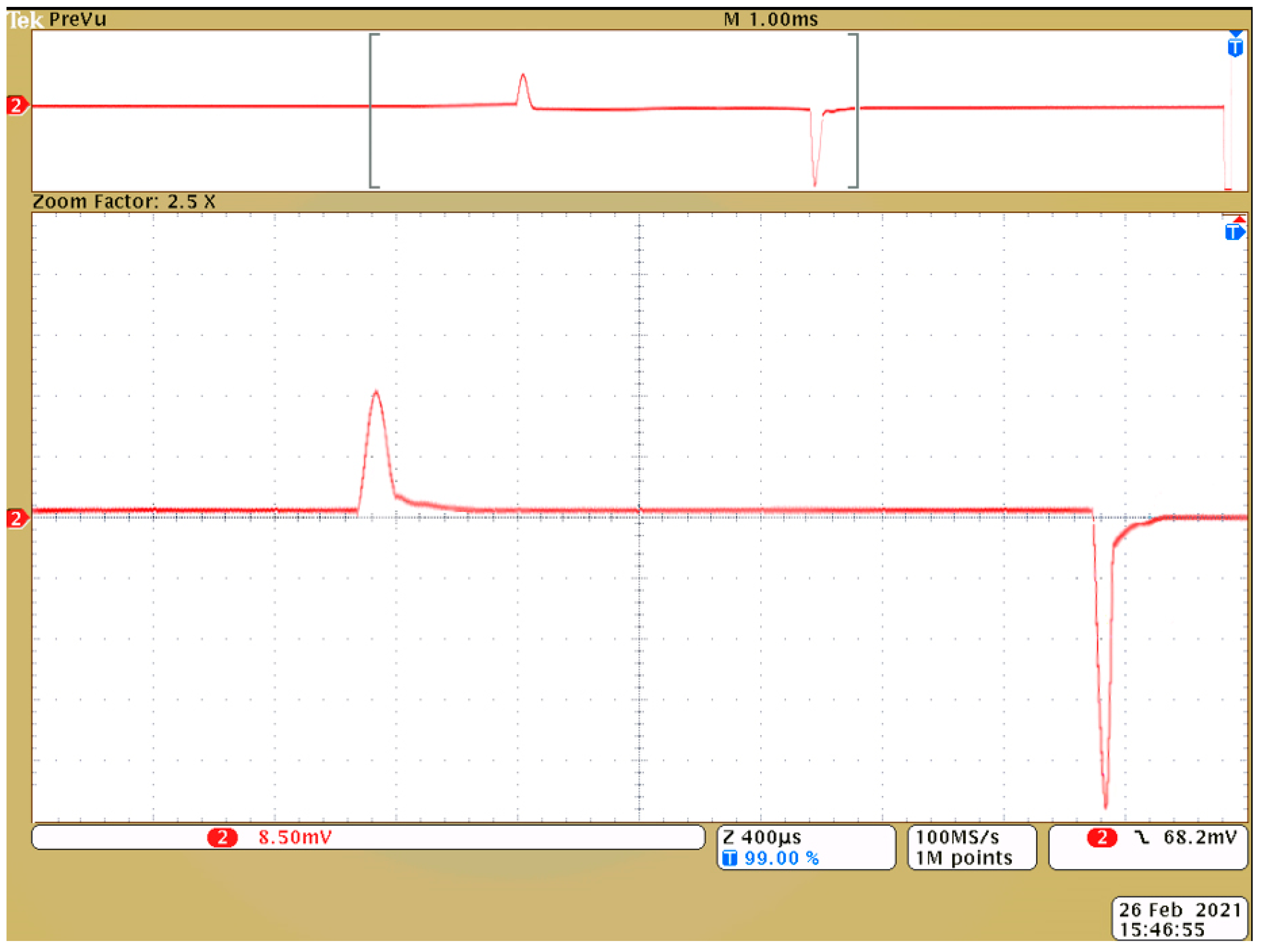
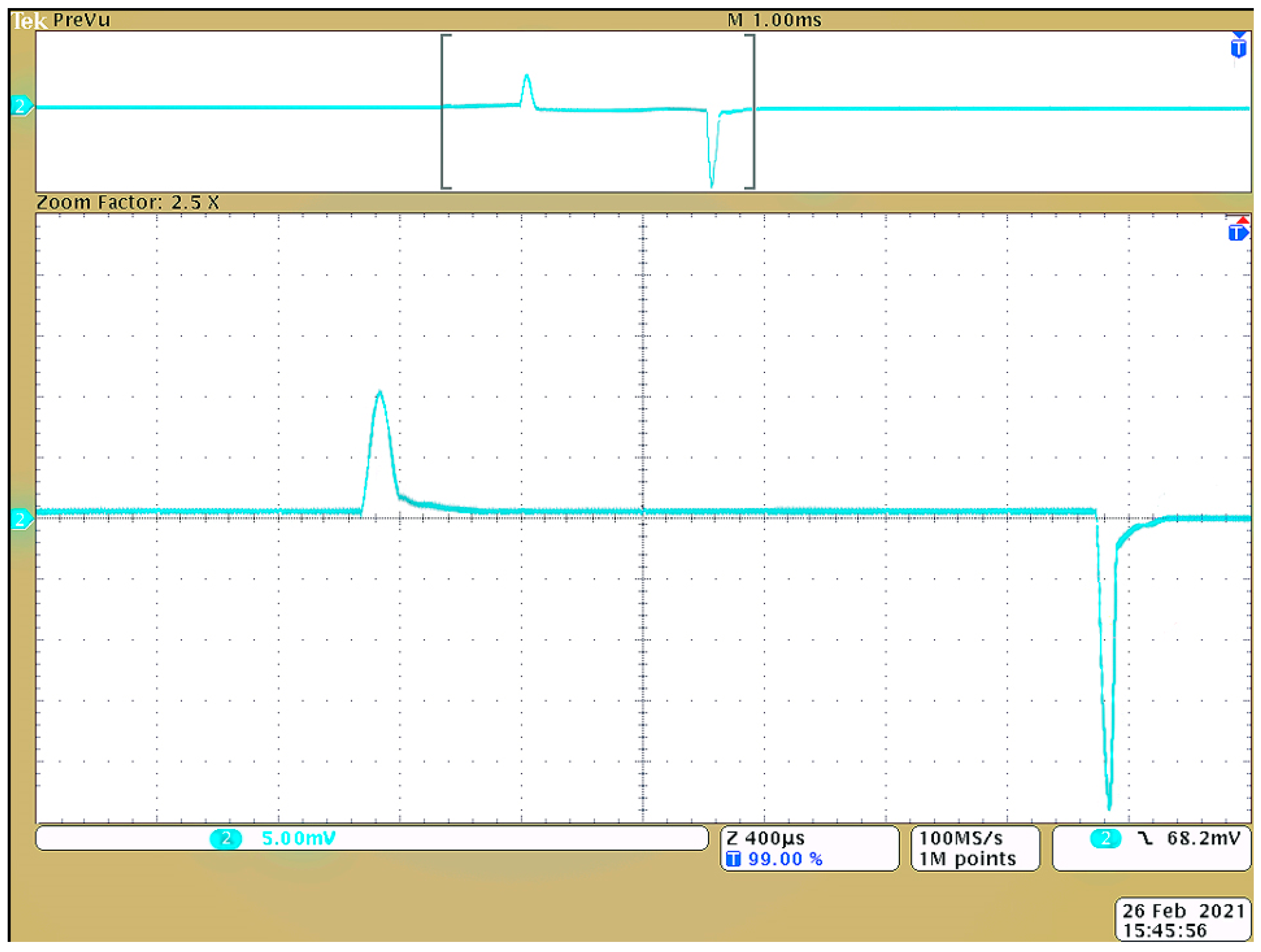
4. Experimental Studies of Spark Discharge

Experimental studies to confirm the advisability of the analyses carried out were carried out using a test stand equipped with a single-cylinder internal combustion engine working with a typical ignition system, as shown in Figure 10. A block diagram of the stand along with the measurement system are shown in Figure 11. The aim of the experiment was to record current oscillograms in the secondary circuit and the voltage generated by the ignition system during the spark discharge.

The experimental verification of the results of digital simulations was carried out with the use of an ignition coil used to generate high voltages in typical ignition systems of spark-ignition internal combustion engines. The tested ignition coil was a system of two induction coils with an open ferromagnetic core of compatible magnetization, the electrical diagram of which is shown in Figure 1. The recorded voltage waveforms u₂(t) and current waveforms i₂(t) are shown in Figure 12 and Figure 13.

As can be seen, the current waveforms i₂(t) and the voltage waveforms u₂(t) obtained from the experiments differ slightly from the results of the numerical experiments shown in Figure 8 and Figure 9.

When comparing the obtained waveforms with the results of the numerical simulations, it should be concluded that the waveforms have similar shapes. The differences between the actual and simulated waveforms are due to the existence of micro capacitances (e.g., between the coil windings) and the absence of a spark plug model in the tested circuit. Completing the circuit model from Figure 1 with capacitive and resistive components and then selecting α and treating the high-voltage wires as a line with distributed parameters in order to reproduce the experimental waveforms as closely as possible will be the subject of the next research [34,35,36]. This will enable obtaining an accurate mathematical description of the circuit under analysis.

5. Conclusions

The path to a mathematical description of reality is led through models based on certain simplifying assumptions. The research indicates that models of electric circuit components in the form of fractional-order models seem to be appropriate. It is often the choice of the correct assumptions (i.e., simplifications) that determines the success of an approach. Therefore, the attempt to eliminate simplifications makes fractional-order calculus particularly applicable in circuit theory as well and can be an excellent tool in the analysis of real systems. In conclusion, it can be stated that the use of fractional-order magnetic coupling between two coils makes it possible to avoid the Dirac impulse that is present in the classical approach. In the case of magnetic coupling of the first order (a classical example), the voltage is assumed to appear immediately and disappear just as immediately (Figure 3)—practically no mechanical or even electronic switch is able to achieve such a state. The use of fractional-order magnetic coupling in this case makes it possible to account for the non-ideality of the coils and the switch. Thus, it provides the possibility to approximate the results of those obtained experimentally in a practical setup. As can be seen, the actual waveforms presented in Figure 12 and Figure 13 are slightly different from the results of the numerical experiments—Figure 8 and Figure 9. The differences between the actual and simulated waveforms are due to the existence of micro capacitances (e.g., between the coil windings) in the tested circuit. An additional conclusion from this research is that the current waveform at the input of the system is the same as for classical coupling and the value of the degree of coupling α greatly influences the value of the voltage induced in the second coil. This means that the larger the value of α, the “stronger” the coupling.

References

1. Nowakowski, W. Układy Impulsowe; WKiŁ: Warszawa, Poland, 1982. [Google Scholar]
2. Hosseini, S.M. The Operation and Model of UPQC in Voltage Sag Mitigation Using EMTP by Direct Method. Emerg. Sci. J. 2018, 2, 148–156. [Google Scholar] [CrossRef]
3. Parsa, N.; Khajouei, G.; Masigol, M.; Hasheminejad, H.; Moheb, A. Application of electrodialysis process for reduction of electrical conductivity and COD of water contaminated by composting leachate. Civ. Eng. J. 2018, 4, 1034. [Google Scholar] [CrossRef] [Green Version]
4. Yu, S.; Tan, Q.; Ives, M.; Liu, M.; Li, L.; Chen, X.; Zheng, M. Parametric Analysis of Ignition Circuit Components on Spark Discharge Characteristics; SAE Technical Paper 2016-01-1011; SAE International: Warrendale, PE, USA, 2016. [Google Scholar] [CrossRef]
5. Stevenson, R.C.; Palma, R.; Yang, C.S.; Park, S.K.; Mi, C. Comprehensive Modeling of Automotive Ignition Systems; SAE Technical Paper 2007-01-1589; Visteon/ACH-LLC, CAE, University of Michigan: Dearborn, MI, USA, 2007. [Google Scholar] [CrossRef] [Green Version]
6. Qisong, W.; Yongping, Z.; Song, L.; Zhiwei, Z. Research on Energy Simulation Model for Vehicle Ignition System. In Proceedings of the IEEE Vehicle Power and Propulsion Conference (VPPC), Harbin, China, 3–5 September 2008. [Google Scholar]
7. Altronic Inc. Advanced Digital Ignition System for Industrial Engines; Altronic CPU-95: Girard, OH, USA, 1996. [Google Scholar]
8. Wang, Q.; Zheng, Y.; Yu, J.; Jia, J. Circuit model and parasitic parameter extraction of the spark plug in the ignition system. Turk. J. Electr. Eng. Comput. Sci. 2012, 20, 2012. [Google Scholar]
9. Sosnowski, M. Modelowanie i Analiza Przebiegu Wyładowania Iskrowego w Silniku z Zapłonem Wymuszonym. Ph.D. Thesis, Akademia Jana Dlugosza w Czestochowie, January 2008. [Google Scholar]
10. Coopmans, C.; Petras, I. Analogue fractional-order generalized memristive devices. In Proceedings of the ASME 2009 International Design Engineering Technical Conferences & Computers and Information in Engineering Conference IDETC/CIE, San Diego, CA, USA, 30 August–2 September 2009. [Google Scholar] [CrossRef]
11. Fouda, M.E.; Radwan, A.G. Fractional-order memristor Response under DC and Periodic Signals. Circuits Syst. Signal Processing 2015, 34, 961–970. [Google Scholar] [CrossRef]
12. Jalloul, A.; Jelassi, K.; Melchior, R.; Trigeassou, J.-C. Fractional modelling of rotor skin effect in induction machines. In Proceedings of the 4th IFAC Workshop Fractional Differentiation and its Applications, Badajoz, Spain, 18–20 July 2013. [Google Scholar]
13. Soltan, A.; Radwan, A.G.; Soliman, A.M. Fractional-order mutual inductance: Analysis and design. Int. J. Circuit Appl. 2016, 44, 85–97. [Google Scholar] [CrossRef]
14. Różowicz, S.; Zawadzki, A.; Włodarczyk, M.; Wachta, H.; Baran, K. Properties of fractional-order magnetic coupling. Energies 2020, 13, 1539. [Google Scholar] [CrossRef] [Green Version]
15. Jesus, I.S.; Machado, J.T.M. Application of Integer and Fractional Models in Electrochemical Systems. In Mathematical Problems in Engineering; Hindawi Publishing Corporation: London, UK, 2012. [Google Scholar] [CrossRef]
16. Martin, R.; Quintana, J.J.; Ramos, A.; de la Nuez, I. Modeling electrochemical double layer capacitor, from classical to fractional impedance. Conf. Pap. J. Comput. Nonlinear Dyn. 2008, 3, 61–66. [Google Scholar]
17. Radwan, A.G.; Fouda, M.E. On the Mathematical Modeling of Memristor, Memcapacitor, and Meminductor; Springer International Publishing: Cham, Switzerland, 2015. [Google Scholar]
18. Petras, I.; Chen, Y.Q. Fractional-Order Circuit Elements with Memory. In Proceedings of the 13th International Carpathian Control Conference (ICCC), High Tatras, Slovakia, 28–31 May 2012. [Google Scholar] [CrossRef]
19. Włodarczyk, M.; Zawadzki, A. Connecting a Capacitor to Direct Voltage in Aspect of Fractional Degree Derivatives. Przegląd Elektrotechniczny 2009, 85, 120–122. (In Polish) [Google Scholar]
20. Podlubny, I. Fractional Calculus: Methods for Applications; XXXVII Summer School on Mathematical Physics: Ravello, Italy, 2012. [Google Scholar]
21. Oldham, K.B.; Spanier, J. The Fractional Calculus: Theory and applications of differentiation and integration to arbitrary order. In Mathematics in Science and Engineering; Academic Press: New York, NY, USA, 1974. [Google Scholar]
22. Podlubny, I. Fractional Differential Equations; Academic Press: San Diego, CA, USA, 1999. [Google Scholar]
23. Caputo, M. Linear Models of Dissipation Whose Q Is Almost Frequency Independent-II. Geophys. J. R. Astron. Soc. 1967, 13, 529–539. [Google Scholar] [CrossRef]
24. Carlson, G.; Halijak, C. Approximation of fractional capacitors (1/s)ˆ(1/n) by a regular newton process. IEEE Trans. Circuit Theory 1964, 11, 210–213. [Google Scholar] [CrossRef]
25. Oustaloup, A.; Levron, F.; Mathieu, B.; Nanot, F.M. Frequency-band complex noninteger differentiator: Characterization and synthesis. IEEE Trans. Circuits Syst. I Fundam. Theory Appl. 2000, 47, 25–39. [Google Scholar] [CrossRef]
26. Krishna, B.T. Studies on fractional order differentiators and integrators: A survey. Signal Processing 2011, 91, 386–426. [Google Scholar] [CrossRef]
27. Różowicz, S.; Tofil, S.Z. The influence of impurities on the operation of selected fuel ignition systems in combustion engines. Archives of Electrical Engineering. 2016, 65, 349–360. [Google Scholar] [CrossRef] [Green Version]
28. Singh, S.N.; Chandler, P.; Schumacher, C.; Banda, S.; Pachter, M. Adaptive feedback linearizing nonlinear close formation control of UAVs. Proceeding of the 2000 American Control Conference, Chicago, IL, USA, 28–30 June 2000; pp. 854–858. [Google Scholar]
29. Zawadzki, A.; Włodarczyk, M. CFE Method—Quality Analysis of The Approximation of Reverse Laplace Transform Of Fractional Order. Prace Naukowe Politechniki Śląskiej. (in Polish). Elektryka 2017, 3–4, 243–244. (In Polish) [Google Scholar]
30. Różowicz, S. The effect of different ignition cables on spark plug durability. In Przegląd Elektrotechniczny; Wydawnictwo SIGMA: Warszawa, Poland, 2018; Volume 94, pp. 191–195. (In Polish) [Google Scholar]
31. Różowicz, S. Use of the mathematical model of the ignition system to analyze the spark discharge, including the destruction of spark plug electrodes. In Proceedings of the 18th International Symposium on Electromagnetic Fields in Mechatronics, Electrical and Electronic Engineering (ISEF), Lodz, Poland, 14–16 September 2017. [Google Scholar]
32. Różowicz, S.; Zawadzki, A. Experimental verification of signal propagation in automotive ignition cables modelled with distributed parameter circuit. Arch. Electr. Eng. 2019, 68, 667–675. [Google Scholar]
33. Różowicz, S. Voltage modelling in ignition coil using magnetic coupling of fractional order. Arch. Electr. Eng. 2019, 68, 227–235. [Google Scholar]
34. Zawadzki, A.; Różowicz, S. Application of input-state of the system transformation for linearization of selected electrical circuits. J. Electr. Eng.-Elektrotechnicky Casopism 2016, 67, 199–205. [Google Scholar] [CrossRef] [Green Version]
35. Zawadzki, A.; Różowicz, S. Application of input—State of the system transformation for linearization of some nonlinear generators. Int. J. Control. Autom. Syst. 2015, 13, 1–8. [Google Scholar] [CrossRef]
36. Szcześniak, A.; Myczuda, Z. A method of charge accumulation in the logarithmic analog-to-digital converter with a successive approximation. Przegląd Elektrotechniczny 2010, 86, 336–340. (In Polish) [Google Scholar]
Figure 1. (a) Model of the ignition system for the simulation studies. Ub—battery voltage, R1—resistance of the ignition coil primary winding, L1—inductance of the ignition coil primary winding, L2—inductance of the ignition coil secondary winding, R2—resistance of the ignition coil secondary winding, R4—resistance representing the losses in the coil core, R3—radioelectrical interference resistance, R34—flow resistance of the spark plug, Rls—discharge resistance, C2—self-capacity of the coil, C34—self-capacity of the spark plug, M—coupling. (b) Substitute diagram of a distributorless ignition system.
Energies 15 00337 g001aEnergies 15 00337 g001b
Figure 2. Block diagrams of the operating stages of the distributorless ignition system (IS); (a) charging the system; (b) discharging the system.
Energies 15 00337 g002
Figure 3. Operator diagram of the ignition system after the voltage is switched on at zero initial conditions.
Energies 15 00337 g003
Figure 4. Voltage waveforms u2(t) at the output of the ignition system for α = 0.9, 0.8, 0.7, and 0.6.
Energies 15 00337 g004
Figure 5. Current waveforms i2(t) at the output of the ignition system for α = 0.9.
Energies 15 00337 g005
Figure 6. Voltage waveform u2(t) at the output of the ignition system for α = 0.9.
Energies 15 00337 g006
Figure 7. Current waveform i2(t) at the output of the ignition system for α = 0.9.
Energies 15 00337 g007
Figure 8. Voltage waveforms u2(t) for the full ignition system operation cycle for α = 0.9, 0.8, 0.7, and 0.6.
Energies 15 00337 g008
Figure 9. Current waveforms i2(t) for the full ignition system operation cycle for α = 0.9, 0.8, 0.7, and 0.6.
Energies 15 00337 g009
Figure 10. Photograph of the test stand.
Energies 15 00337 g010
Figure 11. Block diagram of the test stand.
Energies 15 00337 g011
Figure 12. The recorded oscillogram of the spark discharge voltage waveform u2(t).
Energies 15 00337 g012
Figure 13. The recorded oscillogram of the spark discharge current waveform i2(t).
Energies 15 00337 g013
Publisher’s Note: MDPI stays neutral with regard to jurisdictional claims in published maps and institutional affiliations.