Calculation of Intake Oxygen Concentration through Intake CO₂ Measurement and Evaluation of Its Effect on Nitrogen Oxide Prediction Accuracy in a Heavy-Duty Diesel Engine

Abstract

A new procedure, based on measurement of intake CO₂ concentration and ambient humidity was developed and assessed in this study for different diesel engines in order to evaluate the oxygen concentration in the intake manifold. Steady-state and transient datasets were used for this purpose. The method is very fast to implement since it does not require any tuning procedure and it involves just one engine-related input quantity. Moreover, its accuracy is very high since it was found that the absolute error between the measured and predicted intake O₂ levels is in the ±0.15% range. The method was applied to verify the performance of a previously developed NOx model under transient operating conditions. This model had previously been adopted by the authors during the IMPERIUM H2020 EU project to set up a model-based controller for a heavy-duty diesel engine. The performance of the NOx model was evaluated considering two cases in which the intake O₂ concentration is either derived from engine-control unit sub-models or from the newly developed method. It was found that a significant improvement in NOx model accuracy is obtained in the latter case, and this allowed the previously developed NOx model to be further validated under transient operating conditions.

1. Introduction

Among the different techniques that are currently being investigated to improve the performance and reduce the environmental impact of the transport sector, the model-based control methodology represents an area of interest for both industry and academia. This interest can be confirmed by several studies that have recently been reported in the literature. Some examples are provided in [1,2,3,4,5,6], in which the authors show the advantages of model-based control for several applications, including vehicle speed management, hybrid powertrain energy management and engine management. In [1], the authors proposed a dynamic programming-based optimal speed-planning algorithm for heavy-duty vehicles based on V2X (vehicle-to-everything) communication and look-ahead function. In [2], the authors proposed a predictive driver-coaching system for fuel-economy driving in hybrid electric trucks based on upcoming static-map and dynamic traffic data. In [3], the authors described a hierarchical-model predictive-control framework that can be used to coordinate the power split and the thermal management of the exhaust in diesel hybrid electric vehicles, with the aim of reducing fuel consumption and optimizing the exhaust temperature. In [4], the authors applied a model-based technique to identify the optimal combustion parameters for an 8.42 L diesel engine by exploiting artificial neural networks and polynomial functions. In [5], the authors proposed a real-time physics-based combustion model for diesel combustion to predict the heat release rate, for model-based control purposes. Finally, in [6], the authors conducted a thorough review of model predictive control applications for internal combustion engines and included a discussion on future directions.

Interest in model-based control can also be confirmed by considering the research efforts that have recently been made within such research projects as EU H2020 IMPERIUM, a three-year collaborative project that had the goal of achieving a reduction in the consumption of fuel and urea of about 20% in heavy-duty trucks. The consortium, which was composed of several academia and industry partners [7,8], achieved these results by adopting the following techniques:

• Direct optimization of the control strategy for the main powertrain components (e.g., engine, transmission) to maximize their performance.
• Development of a model-based global powertrain energy-manager supervisor (EMS), which coordinates the different energy sources and optimizes their utilization, according to the current driving situation.
• A more comprehensive understanding of the mission (e.g., eHorizon, mission-based learning) to enable long-term optimization strategies.

In this context, the authors developed a combustion controller that is able to realize specific torque and engine-out nitrogen oxide (NOx) emission targets, as requested by the EMS in real-time, by acting on the injected fuel quantity and on the start of injection of the main pulse [9,10]. The activity was carried out on an 11L heavy-duty diesel engine prototype, which was installed on a vehicle demonstrator.

The developed controller is based on a physics-based 0D combustion model [9] that is capable of simulating the heat release rate, the in-cylinder pressure and the NOx emission formation inside the combustion chamber using a semi-empirical approach [11]. The model was used as a virtual sensor within a control loop to iteratively explore several combinations of the control variables until the predicted torque and NOx emission values were in line with the targets required by the EMS.

The combustion controller was developed and assessed at the test bench during the project [9] and on the vehicle demonstrator on public roads [10].

The controller showed a very good potential for controlling the engine torque under both steady-state and transient conditions. Moreover, the controller was effective in achieving the desired NOx emission targets when the cumulative emissions over transients were considered but was less effective in achieving the desired instantaneous NOx targets, especially for operating conditions in which exhaust gas recirculation (EGR) was adopted [10]. It was speculated, in [10], that the potential sources of errors could be due to either excessive simplifications of the model (such as disregarding the transient thermal effects of the engine) or to inaccuracies of some of the input quantities that were provided to the controller by the engine control unit (ECU), considering that prototypal hardware and software were adopted.

The aim of this study was to verify the latter aspect, in particular concerning the estimation of the oxygen concentration in the intake manifold, which is one of the parameters with the greatest influence on NOx formation [11] and which is therefore a key input variable for the NOx controller in terms of prediction accuracy.

It should be pointed out that the intake O₂ level that was used by the controller as input in the IMPERIUM project was not derived from a sensor, as none was available, but was estimated on the basis of the EGR rate that was provided by the engine control unit (ECU) through its internal sub-models. One of the main objectives of the present study has thus been to investigate the potential improvement of the performance of the previously developed NOx model, which can be obtained when a reliable intake O₂ concentration is provided as input. This allowed the NOx model to be further validated, especially under transient operating conditions.

Since the intake O₂ level was not measured during the transient tests acquired in the IMPERIUM project, and only the experimental intake CO₂ concentration was available, a new procedure was herein developed to derive the former quantity from the latter and from the measured ambient humidity.

1.1. Intake O₂ Estimation: State of the Art and Advantages of the Proposed Procedure

Several studies conducted to estimate the intake O₂ concentration in internal combustion engines have been reported.

In [12,13], the authors evaluated the intake O₂ concentration by correlating it with the ratio between the EGR rate and the relative air-to-fuel ratio and then exploited this correlation to develop an improved air-path controller. In [14], the authors estimated the EGR rate considering the position of the EGR valve and the pressure drop across the valve and then obtained the intake O₂ concentration through the use of a similar correlation to that reported in [12,13]. Alternative methods to estimate the intake oxygen concentration are based on physics-based or artificial intelligence models [15,16,17,18,19,20,21]. In [15], the authors proposed a nonlinear output error model based on artificial neural networks and applied it to a turbocharged diesel engine. In [16], the authors designed and implemented a Luenberger-style nonlinear observer to estimate the intake O₂ mass fraction in a 2.0 L turbo-charged direct-injected gasoline engine. In [17], the authors presented a mean-value modeling approach for a turbocharged light-duty diesel engine. This method can be used to estimate the intake O₂ concentration on the basis of the intake manifold pressure and air flow rate measurements, as well as the exhaust O₂ level. In [18], the authors developed a supervisory model predictive control approach to manage the air path system of a diesel engine under multi-mode operating conditions, where the intake O₂ concentration is modeled and controlled together with the air mass flow rate, the O₂ concentration at the compressor inlet and the pressure drop across the air throttle valve. In [19], the authors proposed a dynamic correction state with extended Kalman filter to improve the performance of intake O₂ estimation methods based on EGR orifice valve modeling. In [20], the authors presented an estimation algorithm based on a first-order linear dynamic model with time varying coefficients in which the necessary input quantities are the boost pressure, the fueling rate, the engine speed and the EGR valve lift. In [21], the authors modeled the in-cylinder oxygen concentration as a function of the ignition delay, which can be obtained by means of the measured in-cylinder pressure, and they applied a Kalman filter to fuse the previous results from the conventional dynamic model with those of the virtual measurements. Finally, in [22], the authors reported a very accurate procedure to estimate the intake O₂ concentration, which was obtained by using a detailed combustion reaction that requires the measurement of all the main chemical species at the engine exhaust, together with the intake CO₂ concentration, as input.

From the previous papers, it emerges that some methods (i.e., [12,13,14]) correlate the intake O₂ concentration with the ratio between the EGR rate and the relative air-to-fuel ratio. Although this correlation is very accurate, a precise estimation of the EGR rate, which may not be easily achievable, especially under transient conditions, is still needed. The EGR rate, in general, is estimated by means of orifice valve models [14], which may be affected by high uncertainties, especially under transient operating conditions [19]. An accurate estimation of the EGR rate requires the simultaneous measurement of the intake and exhaust CO₂ concentrations [22], but this would result in the need to use three input variables to evaluate the intake O₂ level (i.e., the intake/exhaust CO₂ concentrations and the relative air-to-fuel ratio), with the consequent arising of possible issues related to the time misalignment of the acquired signals, especially under transient operation conditions, as well as the combined uncertainty.

With reference to alternative methods based on physics-based or artificial intelligence models (i.e., [15,16,17,18,19,20,21]), they generally require a training procedure on a set of experimental data and may be thus subject to inaccuracies related to variances in the input variables since they generally require more than one input quantity.

Finally, accurate methods, such as that reported in [22], require the measurement of all the main chemical species in the exhaust gases, and this makes it necessary to install a dedicated exhaust gas analyzer.

The procedure developed in this study is instead based on a physics-based approach that requires the use of a single engine-related input quantity (i.e., the intake CO₂ concentration), together with the ambient humidity (which, however, remains quite stable over time). This makes the intake O₂ estimation very robust not only at steady-state conditions but also in transient operation. Moreover, the developed procedure does not require any calibration phase, which makes it easy and robust to implement.

Another advantage of the proposed method is that it allows for a reliable estimation of the intake O₂ concentration to be obtained without the need to install a dedicated sensor at the test bench and using only the measurement of the intake CO₂ concentration and of the ambient humidity, which are commonly acquired for diesel engine testing.

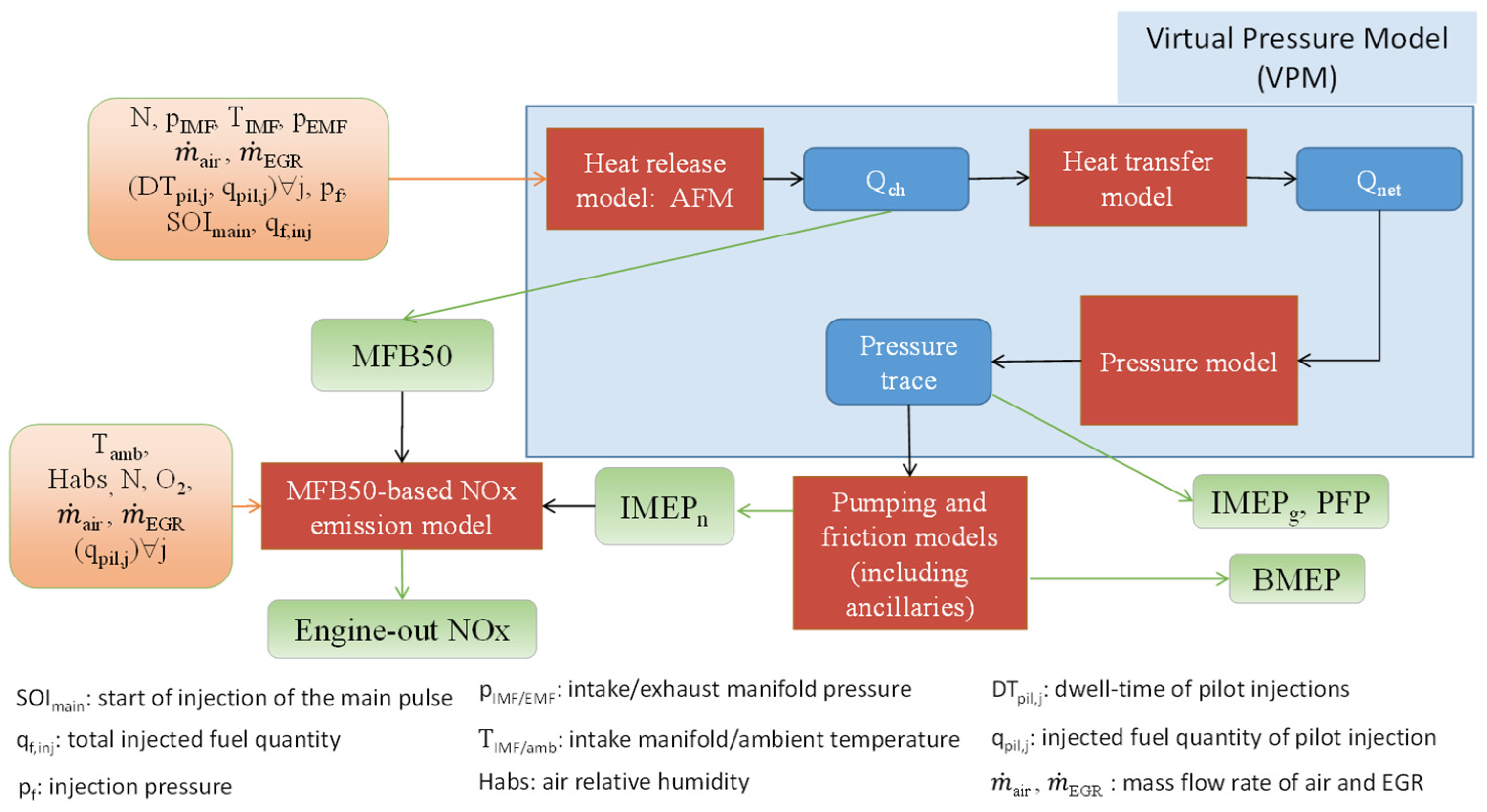
1.2. Summary on the Combustion Controller and Its Performance

A short description of the combustion model and of the combustion controller that was developed during the IMPERIUM project is reported in this section for the sake of clarity.

The schematic of the combustion model is represented in Figure 1.

As can be seen from the schematic, the model first evaluates the chemical energy released by the fuel (Q_ch) on the basis of the accumulated fuel mass (AFM) approach [23,24,25,26,27] and subsequently evaluates the net heat release (Q_net) on the basis of the estimation of the heat transfer to the wall by means of a dedicated sub-model.

The net heat release is then used as input for the pressure model, which is able to reconstruct the pressure evolution inside the combustion chamber over the entire engine cycle. The in-cylinder pressure is set equal to the manifold pressure during the intake and exhaust strokes, and a polytropic evolution is adopted during the compression and expansion phases, while the pressure evolution is evaluated during the combustion phase using the net heat release as input and applying the first law of thermodynamics [28].

Once the pressure trace has been obtained, the indicated mean effective pressure (IMEP_n) is evaluated by integrating the previous quantity over the engine cycle. The pumping losses and the friction losses are then estimated using semi-empirical models (the Chen-Flynn model is adopted for the friction losses [29]), and this allows the brake mean effective pressure (BMEP) to be evaluated, as well as the engine torque.

At this point, the main combustion metrics and parameters, such as the crank angle, at which 50% of fuel mass has burnt (MFB50), and the peak firing pressure (PFP), can be extracted.

The main tuning parameters of the model are derived from correlations, the inputs of which (such as boost pressure, intake temperature, engine speed, etc.) are selected to be representative of the current engine working conditions.

The semi-empirical approach described in [9,11] was adopted for NOx estimation. This model is based on the evaluation of the deviations of NOx emissions with respect to the nominal engine-calibration map values as a function of the deviations of the intake oxygen concentration and MFB50. This approach assumes that NOx formation is closely correlated with combustion phasing, which affects the temperatures of the burned gases, and with intake O₂ concentration [11,30].

The model was first calibrated and assessed in [9] and was then integrated in a control loop in order to set up a combustion controller that is capable of achieving the desired torque and engine-out NOx emission targets in real time.

A conceptual schematic of the controller is reported in Figure 2.

The loop uses the real-time combustion model as a virtual sensor that predicts the actual values of IMEP and engine-out NOx in real time on the basis of the main engine variables, which are provided as input, and then compares the results of the simulation with the required targets. The errors between the values estimated by the model and the targets (i.e., IMEP_error, NOx_error) are then used to correct the values of the control variables (i.e., q_f,_inj, SOI_main), and the iterative loop stops when the errors fall below the defined threshold values (εIMEP, εNOx). When the errors are smaller than the thresholds, the calculated values of the control variables are sent to the ECU to be actuated on the real engine.

The controller was assessed at the test bench using the ETAS ES910 rapid prototyping device to evaluate its capability of achieving the targets.

Several ramps were performed during the testing phase in which the NOx target was varied by a certain percentage with respect to the nominal value in order to evaluate the capability of the controller to reduce/increase NOx levels in real time while satisfying, at the same time, the torque target.

It was found that the controller was able to achieve the torque targets and to increase/decrease the emitted NOx levels when different targets were set (e.g., ±20% with respect to the nominal value), especially when cumulative emissions were considered. However, as previously stated, the controller was less effective in achieving the desired instantaneous NOx targets, especially when EGR was adopted in the engine. Since the EGR rate is an input quantity that is required by the controller to derive the intake O₂ concentration, which, in turn, is needed by the NOx model, it was speculated that the observed lack of accuracy in the NOx control could be ascribed to an inaccurate EGR estimation.

Unfortunately, only the intake CO₂ measurement was available in the performed transient tests, and this could not be used to derive the “experimental” EGR rate to verify this effect. Therefore, a new procedure based on the measured intake CO₂ concentration and ambient humidity was developed in this paper to estimate the oxygen concentration in the intake manifold. The procedure was developed and assessed using steady-state and transient datasets acquired for a 3L diesel engine and applied to the transient tests that had been performed during the IMPERIUM project. This allowed us to verify the potential improvement that could be obtained in the accuracy of the NOx model, especially under transient operating conditions, when a reliable intake O₂ concentration is provided to the model as input.

Section 2 reports a list of the tests that were considered in this work, as well as some details about the analyzers used for CO₂ and O₂ measurements. The new procedure for estimation of intake O₂ concentration is described in detail in Section 3, while the transient tests performed along the IMPERIUM project are simulated again in Section 4 by introducing the intake O₂ concentration evaluated with the new procedure described in Section 3 into the combustion model in order to verify the improvement in terms of NOx prediction accuracy.

2. Materials and Methods

Different experimental tests were considered in this paper. The tests can be divided into two different datasets. The first is composed of steady-state and transient tests, and the second is made up of transient tests. The two datasets can be divided as follows:

4.

Dataset 1: steady-state and transient tests for a 3L diesel engine.

5.

Dataset 2: transient tests for an 11L prototype diesel engine.

The specifications of the engines can be found in [9,10,31].

Dataset 1 was used in this work to assess the new intake O₂ calculation procedure developed in Section 3. Dataset 2 was instead used to evaluate the accuracy of the combustion model in terms of NOx estimation by comparing the cases in which the intake O₂ input is derived either from the EGR rate estimated by the ECU sub-models (baseline case, adopted during the IMPERIUM project) or from the newly developed procedure, which is based on measurement of the intake CO₂ and ambient humidity.

Dataset 1 was acquired at the dynamic test bench of the Politecnico di Torino during previous projects [11] and includes the following tests:

6.

A complete engine map (a total of 123 experimental points were acquired).

7.

An EGR-sweep at some key-points. An EGR percentage of 0 to 50% was explored in these tests, with different levels of trapped air mass (a total of 162 experimental points were acquired).

8.

Sweep tests of the start of injection of the main pulse (SOI_main) and injection pressure (p_f), which were carried out for different key points. SOI_main was varied by ±6 crank angle degrees with respect the nominal values, and p_f was varied by ±20% with respect to the nominal values. A pilot-main injection strategy was adopted (25 experimental points were acquired).

9.

A transient test, which was performed at constant engine speed and while varying the engine load along a “hat-shaped” profile.

A graphical representation of the tests is reported in Figure 3.

Details on the test bench facility used for the acquisition of dataset 1 and on the experimental procedure can be found in [11] and are not reported here for the sake of brevity, but the accuracy and the characteristics of the infrared detector (IRD) and paramagnetic oxygen detector (PMD) sensors used for measurement of the intake CO₂ and O₂ concentration, respectively, are reported in

Table 1. Characteristics of the IRD and PMD sensors.

	IRD i60 CO2 H (High Concentration)	IRD i60 CO2 L (Low Concentration)
Measured compounds:	CO2
Lowest Possible Meas. Range:	0…  0.5%	0…  0.1%
Highest Possible Meas. Range:	0…  20%	0…  6%
T10–90 Time for CO2:	≤1 s	≤1.2 s
T90 Time for CO2:	≤1.5 s	≤1.8 s
Drift:	≤1% full scale/24 h (at typical laboratory conditions, e.g. ambient temperature fluctuations within ±5 °C/41 °F)
Reproducibility:	≤0.5% full scale
Flow rate sample gas:	Approx. 60 L/h
Sample gas condition:	Dew point ≤30 °C (86 °F) Particulates ≤5 μm
	PMD i60 O2
Measured compounds:	O2
Lowest Possible Meas. Range:	0…  0.5%
Highest Possible Meas. Range:	0…  25%
T10–90 Time for CO2:	≤3.5 s
T90 Time for CO2:	≤4.5 s
Drift:	≤1% full scale/24 h (at typical laboratory conditions, e.g., ambient temperature fluctuations within ±5 °C/41 °F)
Reproducibility:	≤ 0.5% full scale
Flow rate sample gas:	Approx. 60 L/h
Sample gas condition:	Dew point ≤30 °C (86 °F) Particulates ≤5 μm
Cross sensitivity	All paramagnetic gases (identical for all paramagnetic sensors)

. The instruments are embedded in an AVL AMAi60 gas analyzer.

Dataset 2 is related to the 11 L diesel engine prototype. Details about the experimental setup can be found in [9]. This dataset was used during the IMPERIUM project to validate the combustion controller under transient conditions.

The dataset includes different load ramps for several engine speed conditions, with and without EGR. Two different load-variation strategies were considered, i.e., variations from 0% to 60–70% of maximum load with intermediate steps (hat-shaped ramp) and variations from 0% to 60% of maximum load with different ramp durations.

A graphical representation of the test types is reported in Figure 4.

The tests performed during the IMPERIUM project involved several repetitions of these ramps, with and without EGR, in which the combustion controller was activated or deactivated. Different NOx targets (nominal, ±20%, −40%) were set for each ramp test when the combustion controller was activated in order to fully assess its functionality. The nominal NOx target levels were identified by resorting to an internally built look-up table, which was a function of the engine speed and load. This table was derived from the measured NOx emissions under steady-state operating conditions over the full engine map, with the baseline configuration of the ECU in order to obtain a “reasonable” NOx target for each engine working condition. A summary of the tests is reported in

Table 2. Summary of the performed tests.

Ramp Test	Engine Speed	Load (Accelerator Pedal Position)	EGR	Combustion Controller	NOx Target When the Combustion Controller Is ON
Ramp test 1	800 rpm	0–60% with intermediate steps	ON/OFF	ON/OFF	Nominal/+20% −20% −40%
Ramp test 2	1300 rpm	0–60% with intermediate steps	ON/OFF	ON/OFF	Nominal/+20% −20% −40%
Ramp test 3	1900 rpm	0–60% with intermediate steps	ON/OFF	ON/OFF	Nominal/+20% −20% −40%
Ramp test 4	1100 rpm	0–60% with different ramp durations	ON/OFF	ON/OFF	Nominal/+20% −20% −40%
Ramp test 5	1500 rpm	0–60% with different ramp durations	ON/OFF	ON/OFF	Nominal/+20% −20%/−40%

.

The capability of the NOx model to increase/reduce the NOx emission levels of a required target along these ramps was evaluated in [9]. In this paper, the ramps were reprocessed by means of the combustion model by providing the intake O₂ level derived from the newly developed procedure as input, instead of the original one, which had been derived from the ECU sub-models. In other words, the ramps were reprocessed using the combustion model as a “virtual sensor”, i.e., by providing the values of the engine state variables as input, as well as of the control variables that had been acquired during the original tests performed during the IMPERIUM project, except for the intake O₂ concentration. This allowed us to evaluate the impact of the intake O₂ concentration on the accuracy of the NOx model under transient operating conditions in order to further assess its validation.

For the sake of clarity,

Table 3. Usage of the experimental datasets in the previous activities and for the present work.

Dataset	Old Usage	Usage in This Paper
Dataset 1 Steady-state tests and transient test for the 3 L diesel engine	Data used for different activities at Politecnico di Torino [11]	Validation of the new intake O2 concentration evaluation procedure
Dataset 2 Transient tests for the 11 L diesel engine	Validation of the combustion controller during the IMPERIUM project [9]	Evaluation of the impact of the intake O2 concentration on the NOx estimation accuracy under transient operating conditions

summarizes the usage of the various datasets in the previous activities and in the present work.

3. Conceptualization of the New Intake O₂ Estimation Method

The conceptualization and description of the new intake O₂ estimation method is reported in this section.

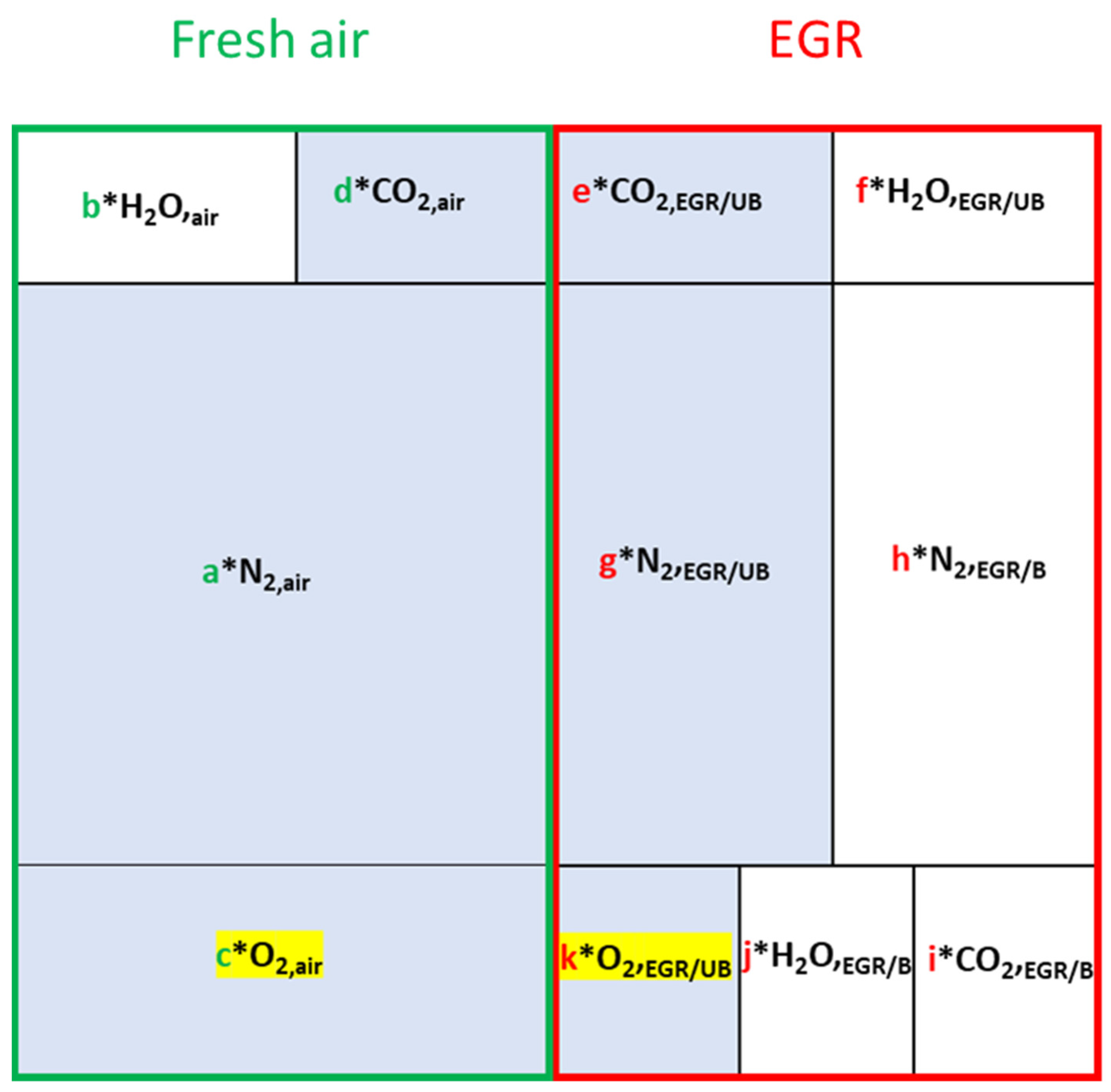
3.1. Description of the General Approach

The proposed method has the aim of estimating intake oxygen concentration by using only the measured intake CO₂ (carbon dioxide) concentration and the ambient humidity.

The method is based on the evaluation of the composition of the charge introduced into the combustion chamber, as reported in Figure 5.

As it is possible to see in the figure, the charge mass introduced into the combustion chamber is split into two contributions: fresh air mass, which is highlighted by the green rectangle, and EGR mass, as highlighted by the red rectangle.

The number of moles of the chemical species for each contribution is indicated in the figure with the letters a, b, …, j.

The fresh air composition includes:

10.

a N₂,_air, which represents the number of nitrogen moles in the fresh air.

11.

c O₂,_air, which represents the number of oxygen moles in the fresh air.

12.

d CO₂,_air, which represents the number of carbon dioxide moles in the fresh air.

13.

b H₂O,_air, which represents the number of water moles in the fresh air due to ambient humidity.

EGR composition is instead split into two contributions, i.e., EGR/B and EGR/UB.

The EGR/B contribution includes CO₂, H₂O and N₂ moles derived from a stoichiometric combustion of dry air with fuel, according to the following reaction [28]:

$$C_x{H}_y+\left(x+\frac{y}{x}\right)\left(O_2+3.773 N_2\right)=xC{O}_2+\frac{y}{2}{H}_{2}O+3.773\left(x+\frac{y}{4}\right)N_2$$

(1)

in which the $\frac{y}{x}$ ratio is set equal to 1.85.

The EGR/B contribution includes the following moles:

14.

i CO₂,_EGR/B, which represents the number of carbon dioxide moles in the EGR contribution due to combustion.

15.

j H₂O,_EGR/B, which represents the number of water-vapor moles in the EGR contribution due to combustion.

16.

h N₂,_EGR/B, which represents the number of nitrogen moles in the EGR contribution due to combustion.

The remaining EGR mass, which is denoted as EGR/UB, represents the EGR contribution from the unburned chemical species (i.e., the species that do not participate in the stoichiometric combustion of fuel with dry air) and represents the excess air that is typically adopted in diesel combustion. The EGR/UB contribution includes the following moles:

17.

e CO₂,_EGR/UB, which represents the number of carbon dioxide moles in the fresh air that is recirculated.

18.

f H₂O,_EGR/UB, which represents the number of water-vapor moles in the fresh air that is recirculated due to ambient humidity.

19.

k O₂,_EGR/UB, which represents the number of oxygen moles in the fresh air that is recirculated.

20.

g N₂,_EGR/UB, which represents the number of nitrogen moles in the fresh air that is recirculated.

The composition of the charge that is introduced into the combustion chamber can be written as follows:

aN_2,air + bH₂O,_air + cO_2,air + dCO_2,air + eCO_2,EGR/UB + fH₂O,_EGR/UB + gN₂,_EGR/UB +
hN₂,_EGR/B + iCO₂,_EGR/B + jH₂O,_EGR/B + kO₂,_EGR/UB = L

(2)

where the a, b, c, d, e, f, g, h, i, j and k indexes represent the number of moles of the related species, and L is the total number of moles of the charge.

The intake oxygen concentration is evaluated, starting from the modeling of the intake charge, which is described above, as the product between the “total volumetric dry-air fraction” present in the intake charge and the oxygen concentration present in the dry air, which is equal to 20.95, as follows:

$$Wet O2int (\%)=Dry Air Fraction\left[\frac{v}{v}\right]\ast 20.95$$

(3)

The total volumetric dry-air fraction can be defined as the sum of all the moles in the blue areas in Figure 5, divided by the sum of all the charge moles, i.e., L, as written in Equation (4):

$$DryAirFraction=\frac{a+c+d+e+g+k}{L}$$

(4)

The volumetric dry-air fraction can also be expressed, taking into account Equation (2), as follows:

$$DryAirFraction=1-\frac{b+f+h+i+j}{L}$$

(5)

It will be shown in the next sections that Equation (5) can be used for the evaluation of the dry-air fraction and therefore of the intake O₂ concentration as a function of the intake CO₂ concentration and ambient humidity.

It should be noted that a wet concentration of the intake O₂ is obtained from Equation (3). This can be verified, for example, by considering the condition in which no EGR is adopted. In this case, the intake O₂ concentration is calculated as follows:

$$Wet O2int=DryAirFraction\left[\frac{v}{v}\right]\ast \frac{20.95}{100}=\frac{a+c+d}{a+b+c+d}\ast \frac{c}{a+c+d}=\frac{c}{a+b+c+d}$$

(6)

which represents the intake O₂ concentration on a wet basis.

The different terms that are necessary to evaluate the intake dry-air fraction, according to Equation (5) (i.e., $\frac{b+f+h+i+j}{L}$), are estimated in the next sections.

3.1.1. Evaluation of the ‘(b + f)/L’ Parameter

The ‘(b+f)/L’ parameter depends directly on the ambient humidity.

The following expression can be derived for the “fresh air” side of the intake charge (see Figure 5) on the basis of the definition of ambient humidity:

$$\frac{\mathit{Habs}}{1000}=\frac{b M_{H2O}}{\left(a+c+d\right)M_{air,dry}}\to \frac{b}{a+c+d}=\mathit{Habs}\ast \frac{29}{18}/1000$$

(7)

where Habs is the measured ambient humidity, expressed in g of water per kg of dry air; 29 is the value adopted for the molar mass of the dry air; and 18 is the molar mass of oxygen.

It is possible to write, for the “EGR side” of the intake charge, that the mass fraction of water, due to the humidity in the intake air, remains the same when the burned gas products are considered. The following expression can be written for a given mass of dry air, m_air,dry, that participates in the oxidation of a mass of fuel, m_f, (thus producing a mass of burned gas m_b):

$$\frac{\mathit{Habs}}{1000}=\frac{M_{H2O} n_{H2O,air}}{m_{air,dry}}~\frac{M_{H2O} n_{H2O,air}}{m_b}=\frac{M_{H2O} n_{H2O,air}}{M_b n_b}~\frac{18 n_{H2O,air}}{29 n_b}$$

(8)

where n_H2O,air represents the number of water moles, due to ambient humidity, that accompanies the dry mass of air m_air,dry, which participates in combustion and which is transferred to the burned mass, m_b. Two assumptions were made in the previous equation. First, the fuel mass, ‘m_f’, was disregarded since m_b was set equal to m_air,dry. This assumption is reasonable for diesel combustion, in which lean combustion is adopted. Moreover, the average molar mass of the burned products (i.e., M_b) was set equal to 29, i.e., that of dry air. This assumption is acceptable since the EGR is composed of “unburned air” and of the stoichiometric burned gases, which feature a molar mass that is not so different from that of fresh air.

Therefore, by considering the last expression in Equation (8) and the EGR composition shown in Figure 5, the following equation can be written:

$$\frac{\mathit{Habs}}{1000}=\frac{18 f}{29\left(e+h+g+i+j+k\right) }\to \frac{f}{e+h+g+i+j+k}=\mathit{Habs}\ast \frac{29}{18}/1000$$

(9)

It is then possible, starting from Equations (7) and (9), to evaluate the ‘(b + f)/L’ factor as follows:

$$b+f=\frac{\mathit{Habs}\ast \frac{29}{18}}{1000}\ast \left(a+c+d+e+h+g+i+j+k\right)$$

(10)

Moreover, by expressing the sum of the moles present in the right side of the equation as the difference between the total mass and the ‘(b + f)’ term, we obtain:

$$b+f=\frac{Habs\ast \frac{29}{18}}{1000}\ast \left(L-b-f\right)$$

(11)

which can be elaborated to obtain the final expression:

$$\frac{b+f}{L}=\frac{\mathit{Habs}\ast \frac{29}{18}}{1000}/(1+Habs\ast \frac{\frac{29}{18}}{1000})$$

(12)

3.1.2. Evaluation of the ‘h/L’, ‘i/L’ and ‘j/L’ Terms

The remaining terms that need to be evaluated to estimate the total intake dry-air fraction are the nitrogen, carbon dioxide and water-vapor mole concentrations derived from combustion, i.e., ‘h/L’, ‘i/L’ and ‘j/L’.

The first concentration that can be evaluated is the CO₂ concentration derived from combustion, which can be derived from the intake CO₂ measurement.

The first step is to define a relation between the measured intake CO₂ concentration and the dry concentration of the charge introduced into the cylinder. In fact, although the CO₂ measured by the analyzer is measured on a “cold” or “dry” basis (since the water present in the burned gases needs to be extracted to avoid any interference with the measuring instrument), some residual water is present in the sampled gas used for the CO₂ measurement, downstream from the cooler. In order to consider this effect, the dry CO₂ concentration can be evaluated, starting from the measured one, as follows:

$$Dry intake CO2=Measured intake CO2\ast \frac{1}{1-H2O_{cooler}}$$

(13)

where $H2O_{cooler}$ is the molar fraction of water that is still present downstream from the gas-analyzer cooler.

The relation between the total dry CO₂ and the CO₂ concentration derived from combustion (‘i/L’) is expressed as follows:

$$\frac{i+d+e}{L-b-f-j}=Dry intake CO2$$

(14)

It can be noted, by analyzing Equation (14), that the ‘i/L’ term cannot be derived directly from the intake CO₂ concentration since that latter also includes the CO₂ ‘(d + e)’ moles that are present in the fresh air and in the air recirculated with the EGR. Moreover, since a dry CO₂ concentration is used, the number of water moles ‘(b + f + j)’ has to be subtracted from the overall number of moles of the intake charge (i.e., ‘L’) in the denominator of Equation (14).

The previous equation can be rearranged to make the ‘i/L’ factor explicit:

$$\frac{i}{L}=Dry intake CO2\ast \left(1-\frac{b}{L}-\frac{f}{L}-\frac{j}{L}\right)-\frac{d+e}{L}$$

(15)

It can be noted, by analyzing Equation (15), that the ‘(b + f)/L’ term is known from Equation (12), but it is still necessary to evaluate the ‘(d + e)/L’ and ‘j/L’ terms.

The ‘(d + e)/L’ term represents the CO₂ concentration in the intake charge that is naturally present in both fresh air and recirculated air. In order to derive this term, it is possible to assume that the mass fraction of the CO₂ that is naturally present in air, the concentration of which is assumed equal to 400 ppm, remains the same when the burned gas products are considered (excluding the CO₂ contribution that is derived from combustion). The following expression can be written for a given mass of dry air, ’m_air,dry’, which participates in the oxidation of a mass of fuel, ’m_f‘, (thus producing a mass of burned gas ‘m_b’):

$$\frac{M_{CO2} n_{CO2,air}}{m_{air,dry}}~\frac{M_{CO2} n_{CO2,air}}{m_b}\to \frac{M_{CO2} n_{CO2,air}}{M_{air,dry} n_{air,dry}}~\frac{M_{CO2} n_{CO2,air}}{M_b n_b}$$

(16)

By assuming that the molar mass of dry air, ‘$M_{air,dry}$’, is equal to the molar mass of the burned gases, ‘$M_b$’, and by using the number of moles of the different chemical species that are included in the fresh air and in the EGR, according to Figure 5, the previous relation can be written as follows:

$$\frac{d}{a+c+d}\left(=\frac{400}{1E6}\right)=\frac{e}{h+j+i+e+k+g}=\frac{e}{L-a-b-c-d-f}$$

(17)

The ‘(d + e)/L’ term can be derived from Equation (17) and, by means of simple mathematical steps, it is possible to obtain the following expression:

$$\frac{d+e}{L}=\frac{400}{1E6}\ast (1-\frac{b+f}{L})$$

(18)

The ‘j/L’ term, which represents the molar concentration of water in the intake charge, as derived from combustion, also needs to be evaluated in Equation (15). This term can be evaluated from the previously shown combustion reaction (i.e., Equation (1)).

It is possible, starting from that relation, to link the concentration of water derived from combustion, i.e., ‘j/L’, with the CO₂ concentration derived from combustion, i.e., ‘i/L’, as follows:

$$\frac{j}{L}=\frac{i}{L}\ast \frac{1.85}{2}$$

(19)

Thus, by replacing Equation (19) in (15), it is possible to write a relation between the intake dry CO₂ concentration and the CO₂ concentration derived from combustion as follows:

$$\frac{i}{L}=\frac{Dry intake CO2\ast \left(1-\frac{b}{L}-\frac{f}{L}\right)-\frac{d+e}{L}}{\left(1+\frac{1.85}{2}\ast Dry intake CO2\right)}$$

(20)

Since all the terms of this expression are known, it can be solved. The terms can, in fact, be derived from the measurements and from Equations (12), (13) and (18).

Once the ‘i/L’ and ‘j/L’ terms have been evaluated, it is possible to calculate the last term that is needed in Equation (5), i.e., the nitrogen concentration, derived from the air that takes part in the combustion in the intake charge (that is, the ‘h/L’ term).

Then, by considering the numbers of water and of carbon dioxide moles derived from combustion (i.e., ‘i’ and ‘j’, see Figure 5), it is possible to evaluate the number of O₂ moles (which is indicated as ‘n_O2b’) that have been involved in the combustion to produce the ‘i’ and ‘j’ moles according to the combustion reaction shown in Equation (1):

$$n_{O2b}=i+\frac{j}{2}$$

(21)

It is now possible to evaluate the number of nitrogen moles associated with the ‘n_O2b‘ moles and transferred to the combustion products as follows.

$$\to h=n_{O2b}\ast 3.773$$

(22)

The ‘h/L’ term is then calculated by means of the following expression:

$$\frac{h}{L}=\frac{n_{O2b}\ast 3.773}{L}=\frac{\left(i+j/2\right)\ast 3.773}{L}$$

(23)

Finally, once the ‘h/L’ quantity is known, it is possible to evaluate the dry-air fraction with Equation (5) and the intake oxygen concentration (on a wet basis) with Equation (3).

Furthermore, if needed, the dry-intake oxygen concentration can be evaluated as follows:

$$Dry O2int=Wet O2int\ast \frac{1}{1-\left(\frac{b+f}{L}\right)-\frac{j}{L}}$$

(24)

The complete procedure is summarized in

Table 4. Summary of the methodology, based on intake CO₂ dry concentration and ambient humidity measurements, used to estimate intake O₂ concentration.

Summary
Intake charge composition: aN2,air + bH2O,air + cO2,air + dCO2,air + eCO2,EGR/UB + fH2O,EGR/UB + gN2,EGR/UB + hN2,EGR/B + iCO2,EGR/B + jH2O,EGR/B + kO2,EGR/UB = L
$\mathrm{Step} 1: \frac{b+f}{L}=\frac{\mathit{Habs}\ast \frac{29}{18}}{1000}/\left(1+Habs\ast \frac{\frac{29}{18}}{1000}\right)$, Habs expressed in gvap/kgair,dry
$\mathrm{Step} 2: \frac{d+e}{L}=\frac{400}{1E6}\ast \left(1-\frac{b+f}{L}\right)$
$\mathrm{Step} 3: \frac{i}{L}=\frac{Dry intake CO2\ast \left(1-\frac{b}{L}-\frac{f}{L}\right)-\frac{d+e}{L}}{\left(1+\frac{1.85}{2}\ast Dry intake CO2\right)}$, $Dry intake CO2 expressed in mol/mol$ $Dry intake CO2=Measured intake CO2\ast \frac{1}{1-H2O_{cooler}}$
$\mathrm{Step} 4: \frac{j}{L}=\frac{i}{L}\ast \frac{1.85}{2}$
$\mathrm{Step} 5: \frac{h}{L}=\frac{\left(i+j/2\right)\ast 3.773}{L}$
$\mathrm{Step} 6: DryAirFraction=1-\frac{b+f+h+i+j}{L}$
$\mathrm{Step} 7: \mathrm{Wet} O2int (\%)=DryAirFraction\ast 20.95$
$\mathrm{Step} 8 (\mathrm{if} \mathrm{needed}): Dry O2int=Wet O2int\ast \frac{1}{1-\left(\frac{b+f}{L}\right)-\frac{j}{L}}$

, which reports the sequence of the calculations that are needed to evaluate the intake oxygen concentration.

4. Results and Discussion

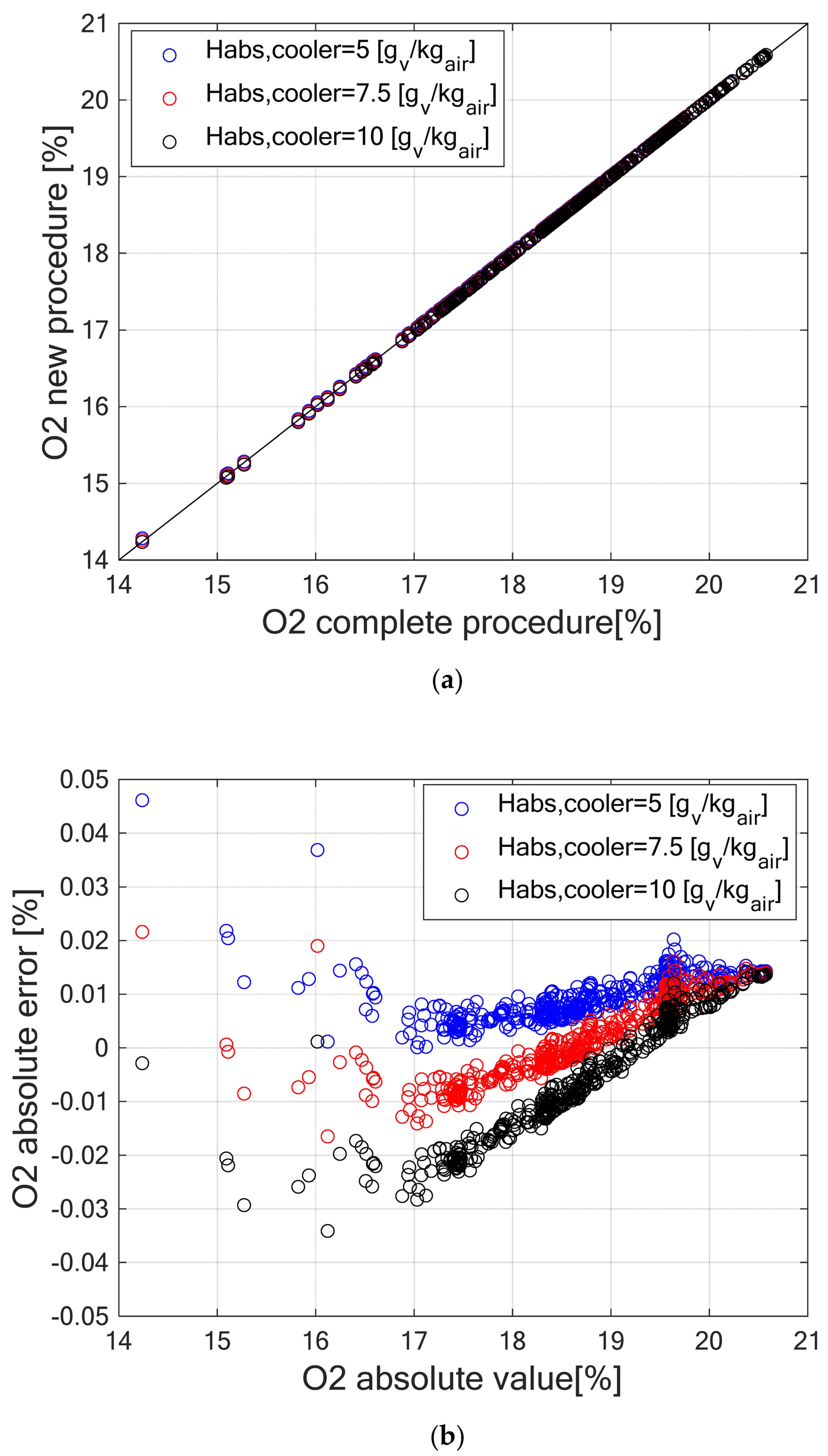
4.1. Validation of the Procedure under Steady-State Conditions

The O₂ model described in Section 3 was first validated under the steady-state conditions of dataset 1. The results of the procedure were then compared with those derived from the methodology reported in [22], which is based on the use of a detailed combustion reaction to evaluate the intake charge composition and requires the measurement of all the main chemical species at the engine exhaust, together with the intake CO₂ concentration. Moreover, the results were also compared with the intake O₂ concentration values that were measured directly by the gas analyzer of the test cell. Such an analyzer usually provides the O₂ concentration on a dry basis.

Two distinct effects should be taken into account for the validation procedure. First, a dry-intake CO₂ concentration has to be used in Equation (14), while the concentration that is measured by the CO₂ analyzer is not completely dry since it is affected by the efficiency of the analyzer cooler (see Equation (13)). Therefore, the residual water molar fraction in the gases exiting the cooler ($H2O_{cooler}$) is a parameter that has to be assumed, and this can lead to a certain degree of uncertainty in the predicted O₂ concentration. Moreover, the O₂ analyzer also provides a concentration of intake oxygen that is not completely dry, which depends on the residual molar fraction of water in the gases exiting the cooler. This effect should also be taken into account when the predicted and measured intake O₂ levels are compared.

In order to take into account these effects, the procedure developed in this paper was applied and validated considering three different levels of $H2O_{cooler}$ in Equation (13) in order to evaluate their impact on the results.

The three considered values of $H2O_{cooler}$ are reported in

Table 5. Values of $H2O_{cooler}$ adopted in Equation (13) for the validation of the procedure and the corresponding H_abs,cooler values in the cooled gases entering the CO₂ analyzer.

H2Ocooler	Habs,cooler [gv/kgair]
0.00868	5
0.0127	7.5
0.0160	10

.

The results of the new procedure were first compared with those obtained using the detailed method described in [22]. The results of the comparison are reported in Figure 6, where Figure 6a reports the intake O₂ concentration values predicted by means of the newly developed method vs. the values obtained using the detailed method reported in [22], while Figure 6b reports the absolute error as a function of the intake oxygen concentration evaluated with the complete method. Both procedures provide a wet intake O₂ concentration.

As it is possible to see in Figure 6, the difference between the values obtained with the proposed procedure and those obtained with the complete procedure described in [22] is very small, and this demonstrates a very good accuracy of the proposed method, despite the fact that it requires only two input quantities, i.e., the intake CO₂ concentration and the absolute humidity of the ambient air.

Moreover, the effect of the $H2O_{cooler}$ parameter does not affect the results to any great extent. Analyzing the results in Figure 6b, it emerges that the use of a value of H_abs,cooler equal to 7.5 g_v/kg_air, which corresponds to a value of $H2O_{cooler}$ equal to 0.0127, seems to provide the best match.

After this preliminary analysis, the results of the new procedure were compared directly with the measured intake O₂ levels provided by the test cell gas analyzer. As previously stated, the analyzer provides a concentration that is not completely dry since it is affected by the residual water present in the sampled gas downstream from the analyzer cooler. Therefore, a correction of the predicted values of the dry-intake O₂ concentration was made for a fair comparison with the measured values.

The first step of such a correction involved the conversion of the wet-intake oxygen concentration, obtained from Equation (3), into a completely dry concentration using Equation (24). The thusly obtained dry-intake O₂ concentration was further corrected to simulate the presence of a certain amount of water in the gas in order to make a fair comparison with the results provided by the analyzer, which are affected by residual humidity resulting from the inefficiency of the cooler.

Therefore, the dry-intake oxygen concentration estimated by Equation (24) (i.e., $Dry O2int$) was further corrected as follows:

$$O2int,corr=Dry O2int \ast \left(1-H2O_{cooler}\right)$$

(25)

where $O2int,corr$ is the predicted intake O₂ concentration, which was corrected to take into account the residual molar fraction of water ($H2O_{cooler}$) that was present in the gases entering the O₂ analyzer.

The results derived from Equation (25) were then compared with those derived from the measurements of the O₂ analyzer, assuming the three values of H₂Ocooler reported in Table 5.

Figure 7 reports the difference between the values of the intake O₂ concentration predicted by the newly developed procedure (corrected with Equation (25) to consider the presence of residual humidity downstream from the analyzer cooler) and the values measured by the O₂ analyzer, as a function of the absolute values of the intake O₂.

Again in this case, it can be seen that the procedure provides very good results, regardless of the residual water-fraction value that is considered, since the maximum absolute error is less than 0.25%. It can also be observed, from Figure 7, that the best matching occurs when a value of H_abs,cooler equal to 7.5 g_v/kg_air is assumed.

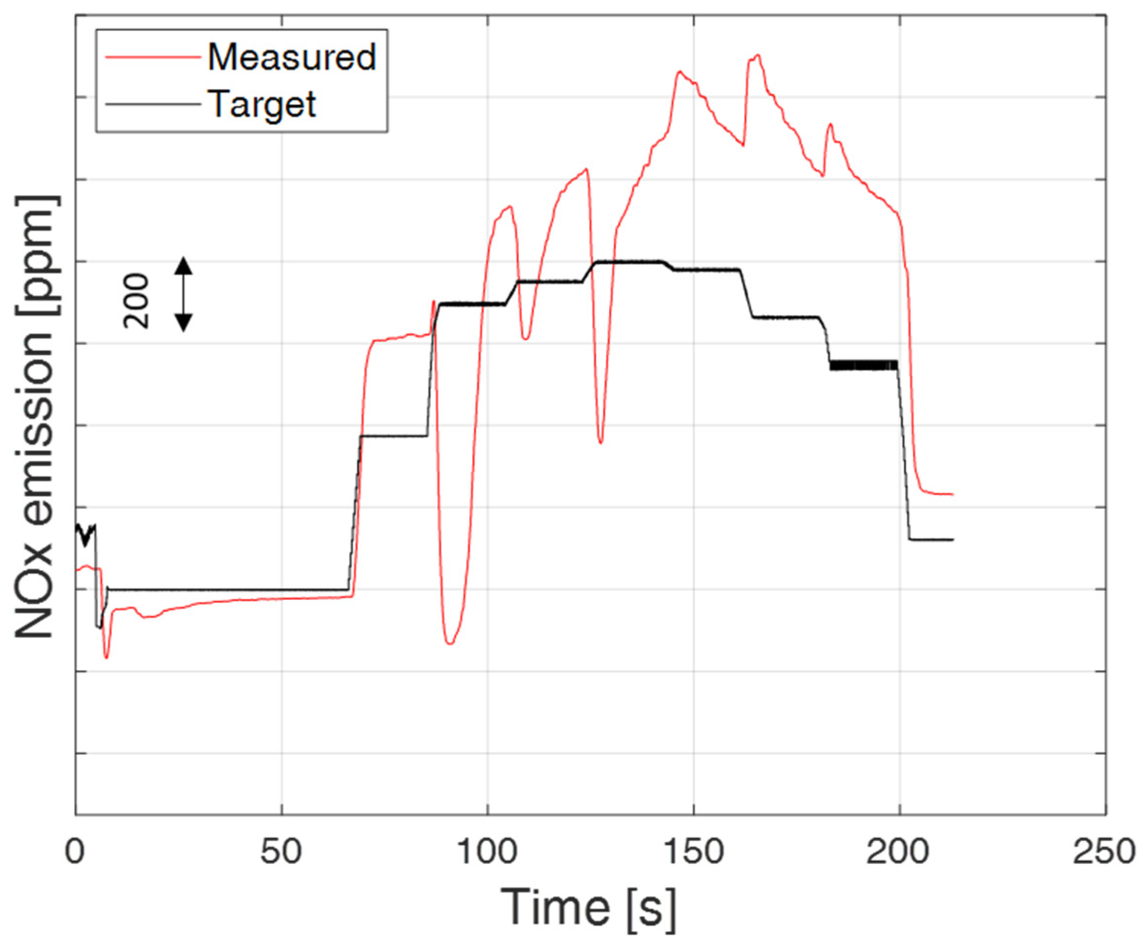
4.2. Validation of the Procedure under Transient Conditions

After the validation of the procedure under steady-state conditions, the accuracy of the methodology was also verified for the transient tests represented in Figure 3b.

Like the previous analysis carried out under steady-state operating conditions, the predicted values of the dry-intake O₂ concentration were corrected using Equation (25) in order to simulate the presence of residual water at the outlet of the gas analyzer cooler. Three different values of H_abs,cooler were assumed (i.e., those reported in Table 5), and the predicted levels of the intake O₂ concentration were compared with the measured levels provided by the test-bench analyzer. The results are reported in Figure 8.

As it is possible to see, the predicted levels of the intake O₂ concentration are in very good agreement with the measured levels, especially whenever a value of H_abs,cooler equal to 10 g_v/kg_air is considered. However, the results can also be considered acceptable when the other two levels of H_abs,cooler are adopted. Therefore, the impact of this parameter on the result is not significant.

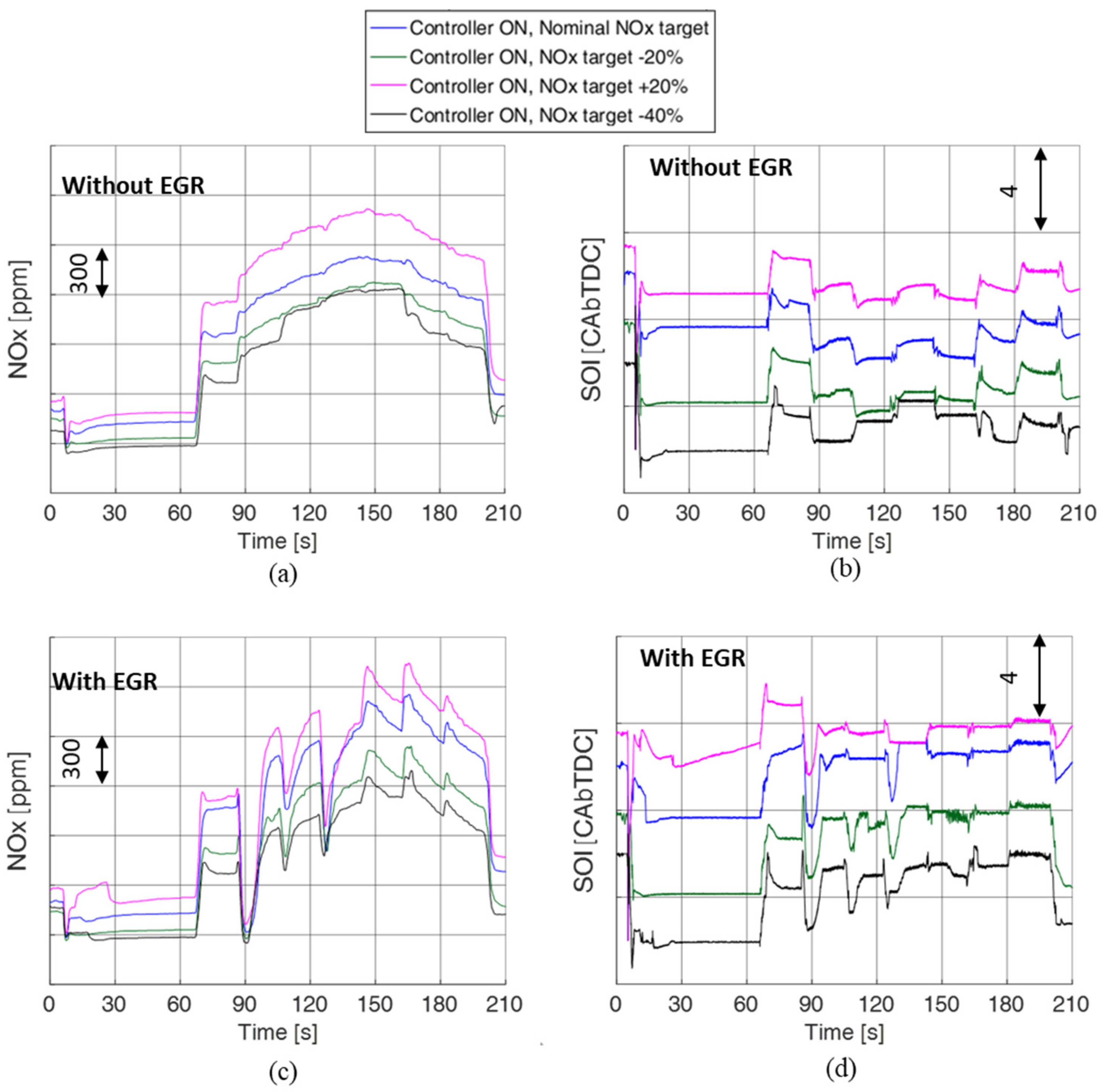
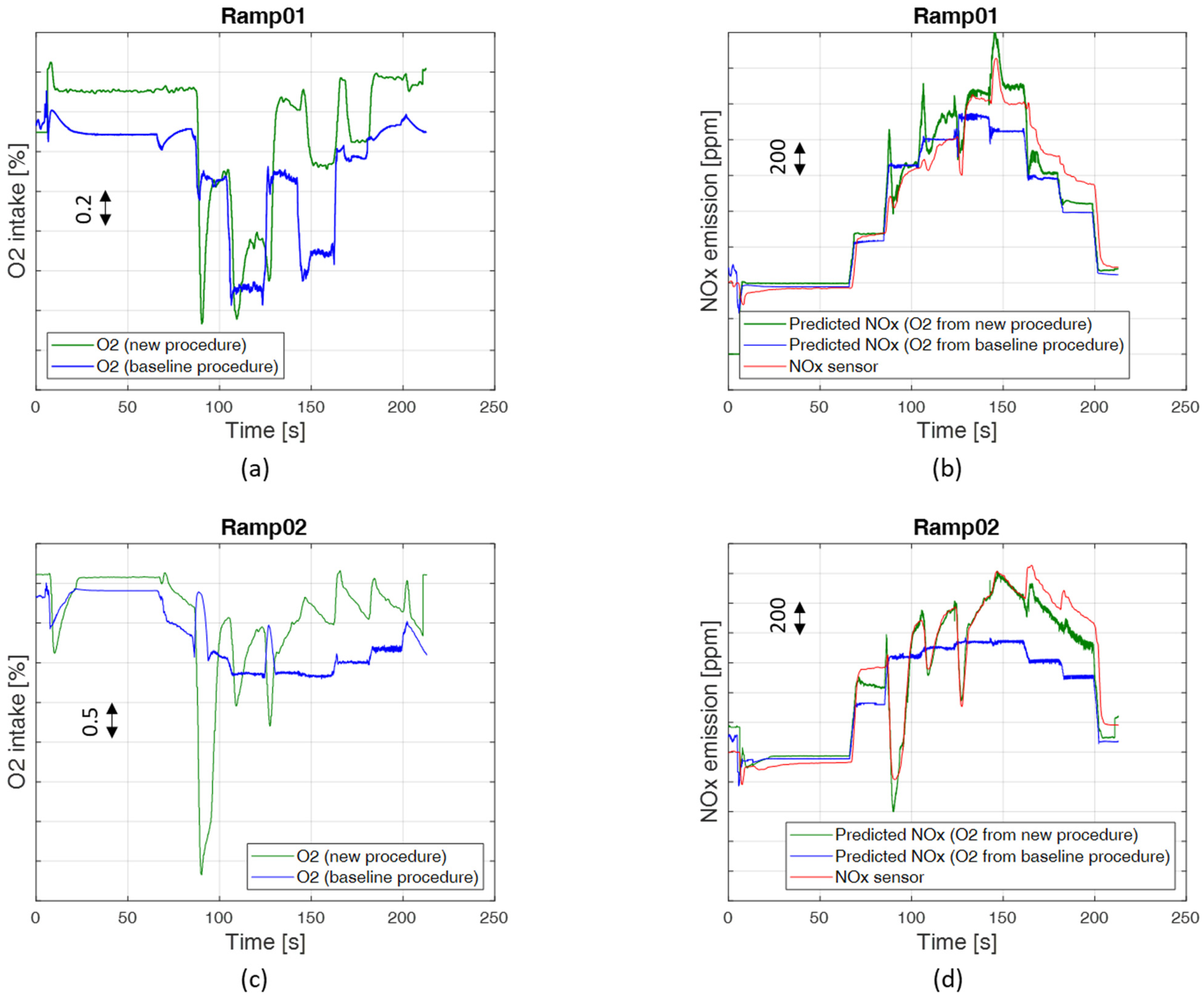
4.3. Validation of the NOx Model Using the Intake Oxygen Concentration Estimated by Means of the New Procedure

After the assessment of the new procedure for the evaluation of the intake O₂ concentration under steady-state operating conditions, the method was applied to the transient tests that were performed during the IMPERIUM project for the 11L diesel engine, that is, those corresponding to dataset 2. This allowed us to verify the improvement in the accuracy of the NOx model that can be obtained, under transient operating conditions, when a reliable intake O₂ concentration is provided to the model as input. In fact, the intake O₂ concentration was not measured during the original acquisition of the ramps, and the intake O₂ level provided to the controller was derived from the EGR rate estimated by means of the prototypal software embedded in the ECU.

As will be shown in the next paragraphs, this approach was able to provide a good NOx control on a cumulative basis but also led to an inaccurate control of the instantaneous NOx levels. However, the intake CO₂ concentration and the ambient humidity were acquired during those tests, and the newly developed procedure for intake O₂ estimation could therefore be applied.

For the sake of clarity, a short explanation of the tests performed during the IMPERIUM project and of the related results is reported hereafter (for further details, the reader may refer to [9,10]).

In short, all the load ramps described in dataset 3 were performed during the IMPERIUM project by activating the combustion controller, and they were repeated several times, either activating or de-activating the EGR system, and by varying the NOx target by fixed percentages with respect to the “nominal” case (i.e., +20%, −20%, −40%). Finally, the results were compared in order to understand whether the controller was effective in increasing/reducing the engine-out NOx levels in real time when different NOx targets were set.

Figure 9 reports, for ramp test 2, the time histories of the measured NOx emissions (Figure 9a,c) and of SOI_main (Figure 9b,d) as examples of the cases in which EGR is either closed or adopted with a nominal level with different NO_x targets.

Four different cases are considered in each chart, i.e.,:

21.

Engine operation with the controller enabled and the nominal NOx target (blue lines).

22.

Engine operation with the controller enabled and the NOx target increased by 20% with respect to the nominal target (magenta lines).

23.

Engine operation with the controller enabled and the NOx target decreased by 20% with respect to the nominal target (green lines).

24.

Engine operation with the controller enabled and the NOx target decreased by 40% with respect to the nominal target (black lines).

The NOx trends shown in the charts were measured by means of the engine NOx sensor.

In general, it can be seen from the charts how the controller progressively advances/delays the start of injection of the main pulse to increase/decrease the engine-out NOx levels.

The percentage differences of the cumulative NOx emissions, with respect to the baseline case with the nominal NOx target, were evaluated and were in line with the target requests (see

Table 6. Ref [10]. Relative differences in the values of the cumulative NOx index, with respect to the baseline case, in which the controller was activated with the nominal NOx target. The underlined values indicated in bold refer to the test conditions in which the boundaries of SOI_main were reached for a significant portion of the test, while the other underlined values indicate the test conditions in which the boundaries of SOI_main were reached but for a limited portion of the test.

Input Type	Controller ON, Nominal NOx Target	Controller ON, NOx Target +20%	Controller ON, NOx Target −20%	Controller ON, NOx Target −40%
Ramp test 1, EGR OFF	Reference	+17.44	−15.77	−26.62
Ramp test 1, EGR ON	Reference	+13.29%	−19.48%	−30.53%
Ramp test 2, EGR OFF	Reference	+21.33%	−16.26	−24.25%
Ramp test 2, EGR ON	Reference	+13.28%	−21.31%	−31.83%
Ramp test 3, EGR OFF	Reference	+21.17%	−18.86%	−28.24%
Ramp test 3, EGR ON	Reference	+19.85%	−22.71%	−35.81%
Ramp test 4, EGR OFF	Reference	+18.99%	−17.89%	−26.41%
Ramp test 4, EGR ON	Reference	+14.03	−14.56%	−28.35%
Ramp test 5, EGR OFF	Reference	+20.44%	−18.51%	−25.44%
Ramp test 5, EGR ON	Reference	+16.39%	−22.07%	−33.62%

, extracted from [10]).

Table 6 reports a summary of the performance obtained in the IMPERIUM project, when the controller was running online, over all the ramp types of dataset 2 [10]. A cumulative NOx index was estimated by integrating the instantaneous NOx concentrations for all the investigated tests. The relative differences in the values of the cumulative NOx index, with respect to the baseline case, in which the controller was activated with the nominal NOx target were then calculated. The underlined values indicated in bold in Table 6 refer to test conditions in which the boundaries of SOI_main were achieved for a significant portion of the test, while the other underlined values indicate the test conditions in which the boundaries of SOI_main were achieved but for a limited portion of the test. When the boundaries were reached, the cumulative values could not achieve the targets, in part due to safety limitations, and therefore, they should not be considered representative of controller accuracy.

As it is possible to see, the combustion controller proved to be effective in increasing/reducing the cumulative NOx emission over a transient test of the required percentage.

However, some discrepancies were found for the instantaneous values of NOx with respect the required instantaneous target.

The ramp test 2, run with the “nominal” NOx target and with an active EGR, is reported in Figure 10 as an example of such discrepancies.

The target values of the engine-out NOx emissions are reported in black, while the red line represents the measured NOx emission levels provided by the engine NOx sensor.

A significant mismatch between the actual and target instantaneous NOx values can be observed in the figure.

It was speculated in [10] that the main cause of this deviation could be related to a non-optimal estimation of the intake O₂ concentration, which was derived from the EGR rate provided by the prototypal software embedded in the engine control unit. The newly developed intake O₂ estimation procedure makes it possible to quantity this effect since the intake CO₂ concentration and the ambient humidity were acquired during the tests.

For this purpose, the combustion model was used as a “virtual sensor” since it was not possible to repeat the tests online with the combustion controller activated, and only the recordings of the acquired tests were available.

The tests were therefore reprocessed offline to the combustion model as input by giving the values of the engine-state variables and of the control variables (i.e., the start of injection of the main pulse and the injected fuel quantity) that had been acquired during the original tests, except for the intake O₂ concentration. The O₂ concentration, which had originally been derived from the ECU-derived EGR rate, was replaced with that derived from the new procedure. At this point, the values of the engine-out NOx emissions predicted by the combustion model were compared with those measured by the NOx sensor installed in the exhaust manifold of the engine.

The whole set of ramps was reprocessed in the same way, except for ramp number 3 because the intake CO₂ concentration was not available for that ramp.

Figure 11 and Figure 12 show the main results of this comparison. Figure 11a,c and Figure 12a,c show a comparison, for the different ramp tests, between the values of the intake oxygen concentration estimated with the new procedure (green line) and the values that had originally been derived from the baseline IMPERIUM procedure in which the EGR rate had been estimated by the ECU (blue lines).

Instead, Figure 11b,d and Figure 12b,d show a comparison, for the different ramp tests, between the NOx values predicted by the model when using the intake oxygen concentration from the baseline procedure (blue lines), the NOx values predicted by the model when using the intake oxygen concentration derived from the new procedure (green lines) and the values of the NOx emissions that were measured by the NOx sensor (red lines).

As it is possible to see from the charts, the use of the intake O₂ concentration values evaluated by means of the new procedure as input for the combustion model allows the estimation of the engine-out NOx emissions to be improved to a great extent for all of the considered ramps.

This suggests that the use of an intake oxygen sensor or the development of an intake O₂ model that is capable of capturing the transient effects in an accurate way could lead to a great improvement in the instantaneous control of NOx emissions.

5. Conclusions

A new procedure based on the measured intake CO₂ concentration and ambient humidity was developed and assessed in this study to evaluate the oxygen concentration in the intake manifold over several datasets for different diesel engines.

The method was assessed under steady-state and transient conditions for a 3 L diesel engine. The main outcomes can be summarized as follows:

-

The new method provides similar results to those obtained from a previously detailed methodology based on a detailed combustion reaction since the difference in the results of the two procedures is in the ±0.01% range.

-

The absolute error between the measured and predicted intake O₂ levels is in the ±0.15% range. It should be noted that the measured O₂ levels are affected by the presence of residual water downstream of the cooler of the gas analyzer. The absolute error of the method is in the ±0.25% range, even when this effect is disregarded.

-

The good accuracy of the method was also confirmed over a transient test.

-

The developed procedure was also applied to verify the performance, in transient operation, of a previously developed NOx model on a heavy-duty 11L diesel engine. It was found that a significant improvement in the accuracy of the NOx model could be obtained with respect to the case in which an ECU (engine control unit)-derived O₂ level was used, when the intake O₂ concentration derived from the new method was given to the NOx model as input.

The main advantages of the proposed method are related to the fact that it does not need any tuning procedure, it requires just one engine-related input quantity and it is very fast to apply and accurate under both steady-state and transient conditions. Therefore, this method is also suitable for engine testing and intake O₂ diagnostic purposes, and it makes it possible to avoid the use of a dedicated sensor.

References

1. Johanssonn, I.; Jin, J.; Ma, X.; Pettersson, H. Look-ahead speed planning for heavy-duty vehicle platoons using traffic information. Transp. Res. Procedia 2017, 22, 561–569. [Google Scholar] [CrossRef]
2. Chen, Y.; Rozkvas, N.; Lazar, M. Driving Mode Optimization for Hybrid Trucks Using Road and Traffic Preview Data. Energies 2020, 13, 5341. [Google Scholar] [CrossRef]
3. Zhao, J.; Hu, Y.; Xie, F.; Li, X.; Sun, Y.; Sun, H.; Gong, X. Modeling and Integrated Optimization of Power Split and Exhaust Thermal Management on Diesel Hybrid Electric Vehicles. Energies 2021, 14, 7505. [Google Scholar] [CrossRef]
4. Wang, H.; Zhong, X.; Ma, T.; Zheng, Z.; Yao, M. Model Based Control Method for Diesel Engine Combustion. Energies 2020, 13, 6046. [Google Scholar] [CrossRef]
5. Samuel, J.; Ramesh, A. An Improved Physics-Based Combustion Modeling Approach for Control of Direct Injection Diesel Engines. SAE Int. J. Engines 2020, 13, 457–472. [Google Scholar] [CrossRef]
6. Norouzi, A.; Heidarifar, H.; Shahbakhti, M.; Koch, C.R.; Borhan, H. Model Predictive Control of Internal Combustion Engines: A Review and Future Directions. Energies 2021, 14, 6251. [Google Scholar] [CrossRef]
7. Imperium Project Information. Available online: http://www.imperium-project.eu/project-information/ (accessed on 12 October 2021).
8. Danninger, A.; Armengaud, E.; Milton, G.; Lütznerc, J.; Haksteged, B.; Zurlo, G.; Schöni, A.; Lindbergg, J.; Krainer, F. IMPERIUM—IMplementation of Powertrain Control for Economic and Clean Real driving emIssion and fuel ConsUMption. In Proceedings of the 7th Transport Research Arena TRA, Vienna, Austria, 16–19 April 2018. [Google Scholar]
9. Finesso, R.; Hardy, G.; Mancarella, A.; Marello, O.; Mittica, A.; Spessa, E. Real-Time Simulation of Torque and Nitrogen Oxide Emissions in an 11.0 L Heavy-Duty Diesel Engine for Model-Based Combustion Control. Energies 2019, 12, 460. [Google Scholar] [CrossRef] [Green Version]
10. Cococcetta, F.; Finesso, R.; Hardy, G.; Marello, O.; Spessa, E. Implementation and Assessment of a Model-Based Controller of Torque and Nitrogen Oxide Emissions in an 11 L Heavy-Duty Diesel Engine. Energies 2019, 12, 4704. [Google Scholar] [CrossRef] [Green Version]
11. Finesso, R.; Hardy, G.; Maino, C.; Marello, O.; Spessa, E. A New Control-Oriented Semi-Empirical Approach to Predict Engine-Out NOx Emissions in a Euro VI 3.0 L Diesel Engine. Energies 2017, 10, 1978. [Google Scholar] [CrossRef] [Green Version]
12. Nakayama, S.; Fukuma, T.; Matsunaga, A.; Miyake, T.; Wakimoto, T. A New Dynamic Combustion Control Method Based on Charge Oxygen Concentration for Diesel Engines. SAE Tech. Pap. Ser. 2003, 1, 3181. [Google Scholar] [CrossRef]
13. Nakayama, S.; Ibuki, T.; Hosaki, H.; Tominaga, H. An Application of Model Based Combustion Control to Transient Cycle-by-Cycle Diesel Combustion. SAE Tech. Pap. Ser. 2008, 1, 850–860. [Google Scholar] [CrossRef]
14. Catania, A.; Finesso, R.; Spessa, E. Real-Time Calculation of EGR Rate and Intake Charge Oxygen Concentration for Misfire Detection in Diesel Engines. SAE Tech. Pap. Ser. 2011, 24, 0149. [Google Scholar] [CrossRef]
15. Malan, S.; Ventura, L. Intake O 2 Concentration Estimation in a Turbocharged Diesel Engine through NOE. SAE Int. J. Adv. Curr. Prac. Mobil. 2021, 3, 864–871. [Google Scholar] [CrossRef]
16. Rengarajan, S.; Sarlashkar, J.; Roecker, R.; Anderson, G. Estimation of Intake Oxygen Mass Fraction for Transient Control of EGR Engines. SAE Tech. Paper Ser. 2018, 1, 0868. [Google Scholar] [CrossRef]
17. Arsie, I.; Cricchio, A.; Pianese, C.; De Cesare, M. Real-Time Estimation of Intake O2 Concentration in Turbocharged Common-Rail Diesel Engines. SAE Int. J. Engines 2013, 6, 237–245. [Google Scholar] [CrossRef]
18. Shin, B.; Chi, Y.; Kim, M.; Dickinson, P.; Pekar, J.; Ko, M. Model Predictive Control of an Air Path System for Multi-Mode Operation in a Diesel Engine; SAE International: Warrendale, PA, USA, 2020. [Google Scholar] [CrossRef]
19. Min, K.; Shin, J.; Jung, D.; Han, M.; Sunwoo, M. Estimation of Intake Oxygen Concentration Using a Dynamic Correction State with Extended Kalman Filter for Light-Duty Diesel Engines. J. Dyn. Sys. Meas. Control 2018, 140, 011013. [Google Scholar] [CrossRef]
20. Diop, S.; Moraal, P.E.; Kolmanovsky, I.V.; van Nieuwstadt, M. Intake oxygen concentration estimation for DI diesel engines. In Proceedings of the 1999 IEEE International Conference on Control Applications, Kohala Coast, HI, USA, 22–27 August 1999; pp. 852–857. [Google Scholar] [CrossRef]
21. Zhang, Q.; Wen, B.; Zhang, X.; Wu, K.; Wu, X.; Zhang, Y. In-Cylinder Oxygen Concentration Estimation Based on Virtual Measurement and Data Fusion Algorithm for Turbocharged Diesel Engines. Appl. Sci. 2021, 11, 7594. [Google Scholar] [CrossRef]
22. D’Ambrosio, S.; Finesso, R.; Spessa, E. Calculation of mass emissions, oxygen mass fraction and thermal capacity of the inducted charge in SI and diesel engines from exhaust and intake gas analysis. Fuel 2011, 90, 152–166. [Google Scholar] [CrossRef]
23. Finesso, R.; Spessa, E.; Yang, Y. Development and Validation of a Real-Time Model for the Simulation of the Heat Release Rate, In-Cylinder Pressure and Pollutant Emissions in Diesel Engines. SAE Int. J. Engines 2016, 9, 322–341. [Google Scholar] [CrossRef]
24. Orthaber, G.C.; Chmela, F.G. Rate of Heat Release Prediction for Direct Injection Diesel Engines Based on Purely Mixing Controlled Combustion. SAE Tech. Paper Ser. 1999, 108, 152–160. [Google Scholar] [CrossRef]
25. Egnell, R. A Simple Approach to Studying the Relation between Fuel Rate Heat Release Rate and NO Formation in Diesel Engines; Society of Automotive Engineers: Warrendale, PN, USA, 1999. [Google Scholar] [CrossRef]
26. Ericson, C.; Westerberg, B. Modelling Diesel Engine Combustion and NOx Formation for Model Based Control and Simulation of Engine and Exhaust Aftertreatment Systems. SAE Tech. Paper Ser. 2006, 1, 0687. [Google Scholar] [CrossRef]
27. Finesso, R.; Spessa, E.; Yang, Y. HRR and MFB50 Estimation in a Euro 6 Diesel Engine by Means of Control-Oriented Predictive Models. SAE Int. J. Engines 2015, 8, 1055–1068. [Google Scholar] [CrossRef]
28. Heywood, J. Internal Combustion Engine Fundamentals; McGraw-Hill Intern: Columbus, OH, USA, 1988. [Google Scholar]
29. Chen, S.K.; Flynn, P.F. Development of a Single Cylinder Compression Ignition Research Engine; Society of Automotive Engineers: New York, NY, USA, 1965. [Google Scholar] [CrossRef]
30. Wu, C.; Song, K.; Li, S.; Xie, H. Impact of Electrically Assisted Turbocharger on the Intake Oxygen Concentration and Its Disturbance Rejection Control for a Heavy-duty Diesel Engine. Energies 2019, 12, 3014. [Google Scholar] [CrossRef] [Green Version]
31. D’Ambrosio, S.; Finesso, R.; Hardy, G.; Manelli, A.; Mancarella, A.; Marello, O.; Mittica, A. Model-Based Control of Torque and Nitrogen Oxide Emissions in a Euro VI 3.0 L Diesel Engine through Rapid Prototyping. Energies 2021, 14, 1107. [Google Scholar] [CrossRef]
Figure 1. Schematic of the baseline combustion model [9].
Energies 15 00342 g001
Figure 2. Schematic of the controller developed during the IMPERIUM project.
Energies 15 00342 g002
Figure 3. Representation of the steady-state tests (a) and the transient test (b) that constitute dataset 1.
Energies 15 00342 g003
Figure 4. Time histories of the accelerator-pedal position for the different ramps acquired at different speeds for the 11L diesel engine.
Energies 15 00342 g004
Figure 5. Graphical representation of the composition of the charge introduced into the combustion chamber.
Energies 15 00342 g005
Figure 6. (a): Wet-intake O2 concentration values predicted with the newly developed procedure vs. the values obtained using the detailed procedure reported in [22] for dataset 1, considering different absolute humidity values in the gases exiting the CO2 analyzer cooler. (b): Error provided by the complete procedure as a function of the intake O2 concentration. The error is evaluated as the difference between the absolute values.
Energies 15 00342 g006
Figure 7. Differences between the values of the intake O2 concentration predicted by the newly developed procedure (corrected with Equation (25), assuming different values of Habs,cooler, in order to consider the presence of residual humidity in the gases exiting the analyzer cooler) and the values measured by the O2 analyzer, as a function of the absolute values of the intake O2.
Energies 15 00342 g007
Figure 8. Values of the intake O2 concentration predicted by the newly developed procedure (corrected with Equation (25), assuming different values of Habs,cooler, in order to consider the presence of residual humidity in the gases exiting the analyzer cooler) and the values measured by the O2 analyzer for the transient test reported in Figure 3b.
Energies 15 00342 g008
Figure 9. Main results obtained in the IMPERIUM project [10]: comparison of the time histories of the measured NOx emissions (a,c) and of SOImain (b,d) for ramp test 2 without EGR (a,b) and with EGR (c,d). The origin of the y-axis is the same in all the figures.
Energies 15 00342 g009
Figure 10. Actual and target values of the engine-out NOx emissions over ramp test 2 with an active EGR and nominal NOx target and with the combustion controller enabled.
Energies 15 00342 g010
Figure 11. (a,c): Time histories of the ECU-derived intake O2 concentration values (blue lines) and of the intake O2 concentration values evaluated by means of the new procedure (green lines). (b,d): Time histories of the engine-out NOx values predicted by the combustion model using the intake O2 concentration derived from the baseline ECU-derived procedure (blue line) and the intake O2 concentration evaluated by the new procedure (green lines), together with the values of NOx emissions measured by the NOx sensor (red lines) for ramp tests 1 and 2.
Energies 15 00342 g011
Figure 12. (a,c): Time histories of the ECU-derived intake O2 concentration values (blue lines) and of the intake O2 concentration values evaluated by means of the new procedure (green lines). (b,d): Time histories of the engine-out NOx values predicted by the combustion model using the intake O2 concentration derived from the baseline ECU-derived procedure (blue line) and the intake O2 concentration evaluated by the new procedure (green lines), together with the values of the NOx emissions measured by the NOx sensor (red lines) for ramp tests 4 and 5.
Energies 15 00342 g012