New Ways for the Advanced Quality Control of Liquefied Natural Gas

Abstract

Currently, gas chromatography is the most common analytical technique for natural gas (NG) analysis as it offers very precise results, with very low limits of detection and quantification. However, it has several drawbacks, such as low turnaround times and high cost per analysis, as well as difficulties for on-line implementation. With NG applications rising, mostly thanks to its reduced gaseous emissions in comparison with other fossil fuels, the necessity for more versatile, fast, and economic analytical methods has augmented. This work summarizes the latest advances to determine the composition and physico-chemical properties of regasified liquid natural gas, focusing on infrared spectroscopy-based techniques, as well as on data processing (chemometric techniques), necessary to obtain adequate predictions of NG properties.

1. Introduction

The increasing number of new natural gas (NG) applications, such as in maritime transport and large trucks, demand faster and more versatile ways to determine its quality. Today, the standardized analytical characterization of the NG composition requires gas chromatography (GC). This is a well-established analytical methodology, capable of measuring accurately and reliably the NG components at very low concentrations (e.g., ca. 0.01% (v/v) [1]). On-line gas chromatographs are currently being implemented for routine measurements and quality control. They are fast (ca. 5 min/sample) but still rely on benchtop instruments for their validation (and frequent revalidation). That is time-consuming and not straightforward. In addition, contractual agreements usually focus on standardized benchtop chromatographs, whose overall running cost per sample is high [2,3,4,5].

In light of the rise of natural gas consumption in the last few decades (though mitigated recently by the COVID-19 pandemic) [6] and the new applications being proposed [7], it is expected that NG production will keep increasing for, at least, the next two decades [8], even considering the most optimistic predictions for the use of renewable energies.

This favors the development of new, faster, and versatile quality control methods. Some of them are based on physical measurements, such as combustion energy, speed of sound, or density, and they have been applied to determine the heating value [9], the lower heating value plus the Wobbe index (WI), and the stoichiometric air–fuel ratio [10], as well as the Methane number, WI, and CH₄, C₂H₆, and CO₂ concentrations [5,9,10,11]. Noteworthy, these methods require complex instrumentation.

Small electrochemical sensors offer a very appealing and convenient solution (likely, portable in a near future) for routine measurements, although they are still under development and have not been commercialized. Some of them are based on capacitive transducers whose signals depend on the presence (and quantity) of specific NG compositional gases [12,13,14].

In addition, different kinds of convenient spectroscopic measurements (although not fully portable, still) were proposed for NG quality control, mostly based on the use of infrared radiation [3]. They ranged from tunable-filter near infrared radiation [12] to common Fourier transform IR spectrometry (FTIR), both in the near region (NIR, 12500–4000 cm⁻¹, [15,16] because it contains the 1st and 2nd overtone regions –5700 and 8300 cm⁻¹, respectively, plus the 1st overtone of the combination mode of hydrocarbons, 7150 cm⁻¹), and in the medium region (MIR, 4000–450 cm⁻¹). Although NIR was initially suggested as an optimal spectral region, this has been shown not to be the case always and MIR provided very advantageous, as well [2].

Raman spectrometry has also been suggested to measure the chemical composition of gases [4,17,18] and was applied to evaluate the composition of NG and biogas [19] and fuel gas [20] (from CH₄ to C₄H₁₀).

It is worth noting that several difficulties arise when using IR and Raman spectrometry. In effect, as NG is composed of a variety of molecules, the resulting spectra are a complex combination of overlapping peaks and/or broad bands corresponding, more often than not, to several compounds (for example, the peaks around 2950 cm⁻¹ correspond to the C-H stretching vibrational mode, which belongs to every aliphatic molecule in the gas). The use of chemometric methods has been demonstrated to be useful to circumvent this problem [2].

The main objective of this work is to offer tutorial guidelines on how to develop an advanced MIR-based quality control methodology to estimate NG quality control parameters. The approach detailed here is based on measuring gaseous infrared spectra of regasified liquefied natural gas (LNG) and coupling them with multivariate statistical modeling. Details are given on the experimental setup used to gather reliable results and the workflow to get a sound prediction model.

2. Materials and Methods

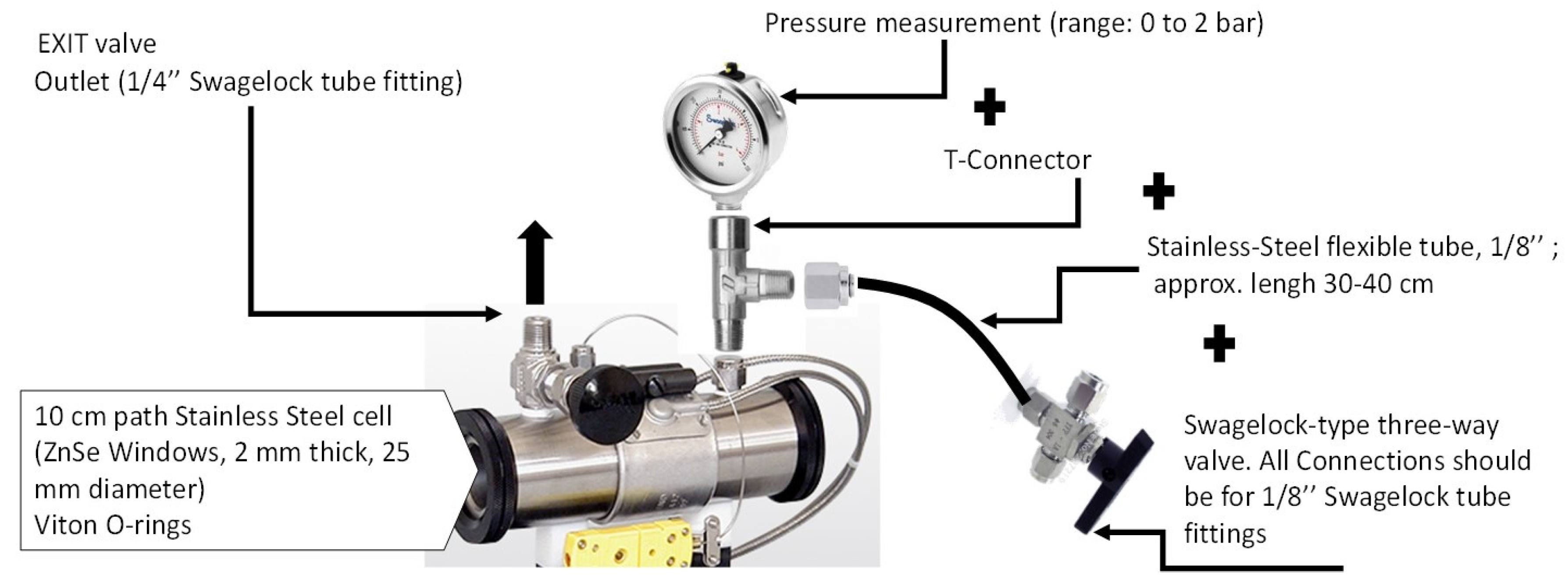
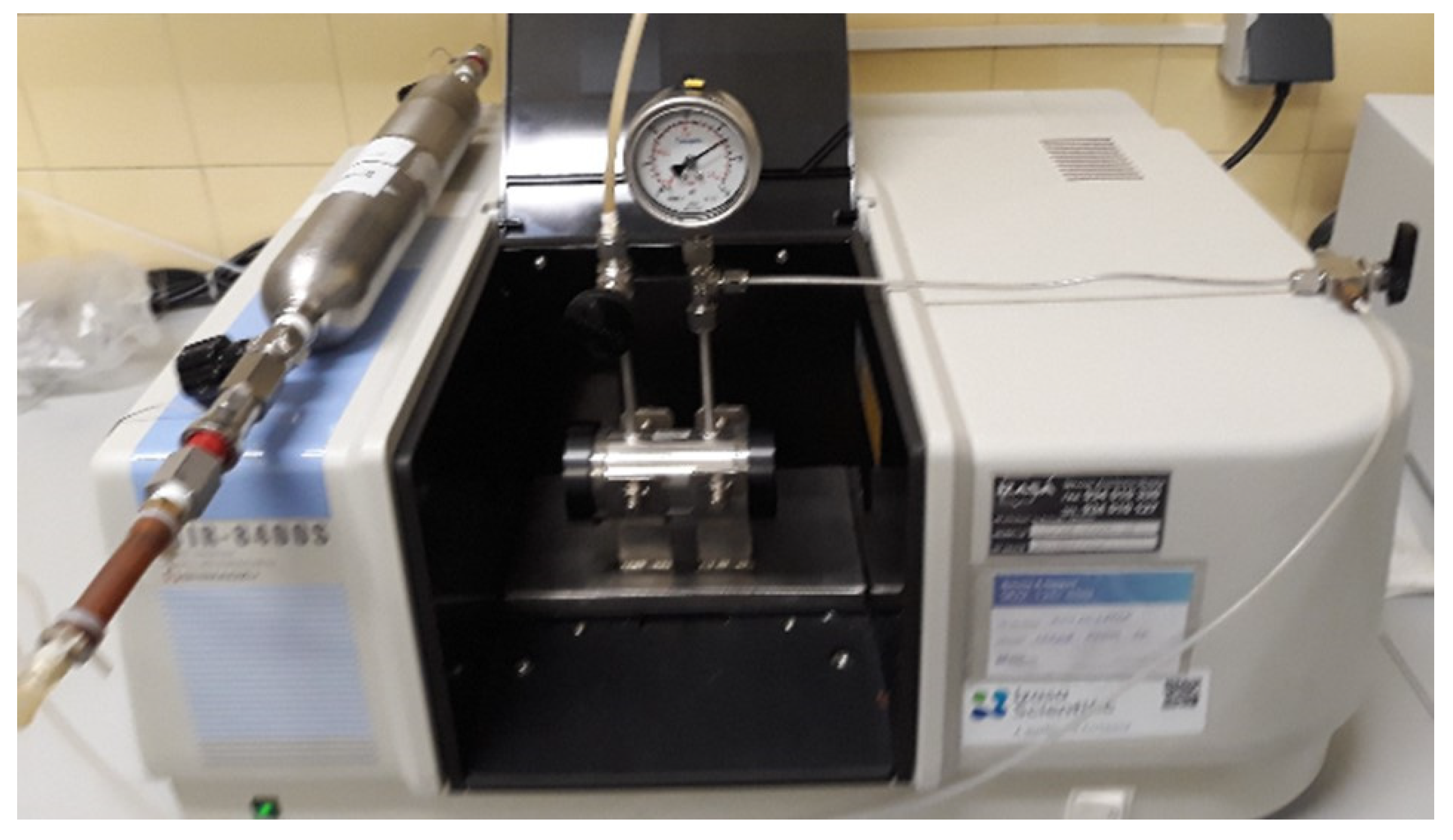
2.1. Instrumentation

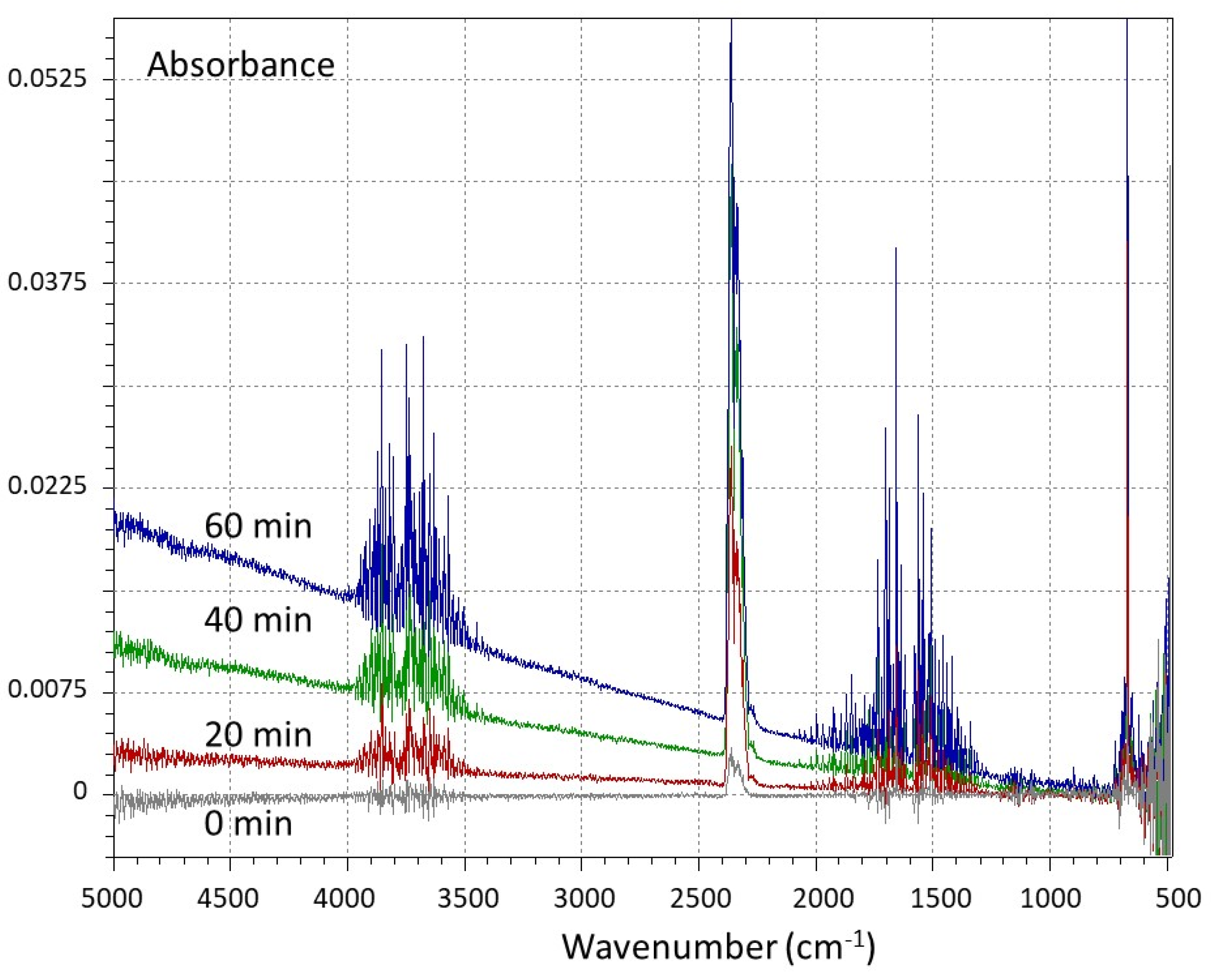
A relevant issue when analyzing NG is the gas cell. The most important factors defining it are the pressure it can withstand, the optical length, and the material of the windows. The first may affect the seals and the cell windows since an excessive pressure may cause leaks and damage the usually expensive and fragile cell crystals (windows), also creating security concerns, as NG is flammable. In our experience, a sample pressure around 0.2 bar is enough to obtain well-defined spectra, although the signals are improved using additional an inert gas, as explained in Section 2.2.

The optical path impacts directly on the intensity of the spectral peaks (so, on the Lambert-Beer-Bouguer’s law). Single-pass, multireflection, and hollow-core fiber cells can be used to study NG. The first type is very straightforward, as it only consists of a capsule (the simplest one made of glass) with IR-transparent windows, which the IR beam traverses linearly. Such a cell tends to be not very long, often not exceeding 10 cm, thus yielding a relatively short optical pathlength. More robust 10-cm single-pass cells are of stainless steel and might be thermostatized, as well [21,22,23].

Multireflection cells contain a series of internal mirrors that reflect the IR incident beam, augmenting the pathlength. The limiting factor in these cells is the reflection coefficient of the mirrors, which determines the maximum number of reflections. Typical pathlengths can range between 1 and 15 m [21,22,23,24].

A hollow-core fiber cell consists of a hollow internal-reflection fiber filled with the gas (Figure 1). A laser beam (usually from a quantum cascade laser [25]) is focused on the hollow core space and travels inside the coil to the detector, with a pathlength equal to the longitude of the fiber. The main limitation is the loss of energy in the beam as it travels through, which is affected by both the length and the curvature of the fiber [24]. Typical pathlengths are between 0.1 and 5 m. Even though there have been some studies with methane samples [26], hollow-core fibers are not still of common usage; so, we will focus on traditional cells.

At first, multireflection cells may appear as a good choice because of the many reflections they have, which increase the S/N (signal to noise) ratio. However, they might not be the best option, as they are very expensive and need large sample quantities, not only for the measurement itself but for the previous purge required to avoid cross-contamination. In addition, major sample components might be an issue because their signals can saturate the spectrum. In addition, those cells are quite fragile because of their glass body, and the mirrors need regular realignment (not difficult, but time-consuming).

Figure 2 compares two spectra of a regasified LNG sample measured with a 10 cm pathlength single-pass cell and with a 1 m pathlength multireflection cell. It can be seen that even though the intensity is considerably higher for the latter (indeed, too high, with absorbances up to 2.5), the general spectral profiles are identical, and no peaks were lost when the short cell was used.

Nevertheless, for a simple and straightforward working protocol, the single-pass cell can (and should) be customized so that the filling and emptying of the cell become simple, and the backgrounds are recorded easily. Figure 3 shows an example that we have used quite successfully. It consists of a 10 cm path, stainless steel Harrick gas cell (Harrick Scientific, Pleasantville, NY, USA) with 2 mm-thick, 25 mm-diameter ZnSe windows, an input tube with a Swagelock 3-way valve, an exhaust tube, and an internal pressure gauge.

As for any traditional IR application, the material of the windows is a very important parameter, as it can reduce the range of wavenumbers in which the analysis can be performed. This is also exemplified in Figure 2. The spectra obtained for the short cell with ZnSe windows is well defined in the 500–950 cm⁻¹ region, which is totally obscure when CaF₂ windows were used in the multireflection cell. This region is relevant when studying hydrocarbons. For the sake of information, the most common window materials are summarized in

Table 1. Some common gas cell window materials and their transmission working range [27,28,29] (there may be slight discrepancies in the wavenumbers among the references).

Window Material	Effective Range (cm−1)	Window Material	Effective Range (cm−1)
AgCl	25,000–360	KBr	40,000–340
AMTIR (GeAsSe)	11,000–625	KRS-5 (TlBr + TlI)	16,600–250
BaF2	50,000–740	NaCl	40,000–625
CaF2	50,000–1025	Sapphire (Al2O3)	50,000–1525
Chalcogenide (AsSeTe)	4000–900	Si	8000–660
CsI	33,000–200	SiO2	50,000–2500
Diamond	40,000–12.5	ZnS	17,000–690
Ge	5500–475	ZnSe	10,000–550

, along with their effective wavenumbers working ranges [27,28,29].

When selecting an instrument to perform IR measurements several important parameters need to be addressed. A first factor to take into consideration is the wavenumbers range, ideally from 5000 to 450 cm⁻¹ so it includes the 3rd methane overtone around 4400 cm⁻¹ and the aliphatic C-C skeletal vibrations around 600 cm⁻¹. A basic setup might be the one depicted in Figure 4, with a Shimadzu 8400S Spectrometer (Shimadzu, Kyoto, Japan) and the gas cell depicted in Figure 3.

A second issue is the nominal spectral resolution. In gas analysis, this is a particularly relevant parameter as gas spectra contain very narrow rotovibrational peaks very close to each other. Resolution can be defined as the wavenumber interval at which two consecutive datapoints are recorded. A high resolution means small intervals (closely adjacent intensity signals), more data, well defined spectra, and less overlap between peaks. However, it also decreases the speed of the analysis and reduces the S/N ratio, which implies that a higher number of scans is required to get a satisfactory spectrum [30]. A minimum 1 cm⁻¹ resolution is required to resolve the signals; otherwise, the spectral bands will overlap in excess (see Figure 5). Such a resolution is easily attainable by most modern FTIR instruments, and they even offer much better ones (current benchtop instruments offer up to 0.25 cm⁻¹ resolution). However, one must be sure that the wealth of data per spectrum can be retrieved and saved fast (more than 15,000 digitized values per spectrum for highest resolutions) and handled by statistical software, which is not always the case. So, depending on the available instruments and computers, a compromise might be needed.

There are more thorough definitions of resolution, based on the Rayleigh or the full width at half-height (FWHH) criteria. The Rayleigh criterion states that two adjacent spectral lines (with a sinc²(x) form and equal intensity) “are considered to be just resolved when the center of one line is at the same frequency as the first zero value of the other” [31]. Visually, a slight drop (approximately 20%) between the two maxima can be seen. On the other hand, the FWHH criterion states that two triangular shaped lines are resolved when the spacing between the lines is greater than the FWHH of either line [31]. This latter definition, however, is not very appropriate for FTIR devices [31]. The nominal resolution is going to affect the required time of analysis, so a trade-off between time and quality of the spectra must be obtained.

A third issue is the number of scans recorded by the instrument to get the final spectrum. It influences the time required to retrieve the final spectrum, as well as its quality. As for any instrumental device, there is always a certain degree of variability in the signal due, in part, to the motion of the gaseous molecules in the sample, which causes many IR bands/peaks to be of low intensity [30], but also due to instrumental noise [32,33]. Too few scans will yield a spectrum with a poor S/N ratio, whereas a high amount of scans helps in removing this variability by averaging out random noisy signals, thus offering a more precise result. However, recall that noise gets only reduced by a factor of 1/√n (n = number of scans) [32,33]. The optimal number of scans depends on several factors, such as the physical state of the sample (gases need more scans than solids), temperature control of the room, externally caused bench vibrations, real-time processing capabilities of the microprocessors, etc. In our experience (room temperature controlled to ±1 °C), around 200 scans per spectrum offer an optimal result, though 100 scans yielded suitable final spectra many times.

A well-known point for all IR practitioners is the need to background-correct the spectra. However, the stressing environment of industrial laboratories, with tight delivering times, much workload, and adjusted personnel, may tempt analysts to measure gas samples in a ‘continuous mode’ without recording new backgrounds. Now, taking into account that 200 scans (1 sample) need ca. 15 min to be recorded (this obviously depends on the instrument being used and the number of scans and resolution), it is clear that the atmosphere of the laboratory is prone to fluctuate; thus, the background after 15, 30, … min will definitely not be constant. Therefore, it is critical to perform a background before every sample is measured, especially whenever extensive recording times are needed. Failure in doing so will lead to ‘tilted’ spectra and more intense peaks associated to environmental water, CO, and CO₂ (at least, but any organic volatile solvent from the laboratory can also be detected). This will be more dramatic as time goes by (Figure 6) and becomes very important as soon as after 60 min. A way to avoid this is to tightly close the space where the gas cell was installed and continuously purge with N₂, which is not always feasible as it happens in Figure 4.

Finally, apodization is a mathematical operation applied after the Fourier transform that minimizes the appearance of secondary peaks at both sides of the actual peak [34]. For natural gas analysis, medium-strong functions, such as Happ-Genzel or Beer-Norton, are used commonly. The strongest the function is, the lower the secondary, undesired, peaks are, but, also, the required signal of interest decreases, as well. To select the best level of apodization preliminary trials have to be performed considering the various possibilities of the instrument-controlling software. Different vendors offer different algorithms, although the ‘strong’ functions are good many times. It is recommended to report the apodization function applied in your particular study and maintain the selection throughout all the measurements.

2.2. Gas Broadening

A typical problem when measuring LNG is that the product contains major constituents (>75%, v/v concentrations, e.g., methane) and minor components (<1%, v/v concentrations, e.g., butanes and pentanes), all of them being of importance for quality control purposes. Hence, there is some difficulty in obtaining representative signals for each compound, despite the overall spectrum has visually nice characteristics (low noise, well-shaped bands, etc.). A way to address this problem consists of boosting the less intense bands using a so-called broadening gas (or filling gas). That consists of an inert gas that, when added to the gas sample, enhances the signal of weakest peaks. The effect has been known since the first half of the 20th century [35,36,37] but not too applied in routine quality control measurements. Briefly, the molecules of the inert gas collide with those of the sample compounds, momentarily blocking the rotation of the atoms in the moment of the collision. This enhances the analytical signal of the rotational modes, increasing the intensity of the spectral peaks.

The operational procedure when dealing with a broadening gas is not difficult and we found nice results considering the next steps [38]: (i) purge the cell with the filling gas (0.5 bar, 1 min); (ii) record background; (iii) purge with a small flow of the sample gas; (iv) fill the cell with the sample (0.2 bar), and, then, add the broadening gas until a total pressure of 1.5 bar; and (v) record spectra.

In previous studies [38] a suite of inert gases (N₂, He, and Ar) was evaluated to determine which improves most the sensitivity of selected weak bands when measuring commercial LNG samples. Out of them, Ar arose as the most adequate one to enhance the low intensity peaks (as shown in Figure 7), while N₂ and He just increased the signal of the overall spectra equally.

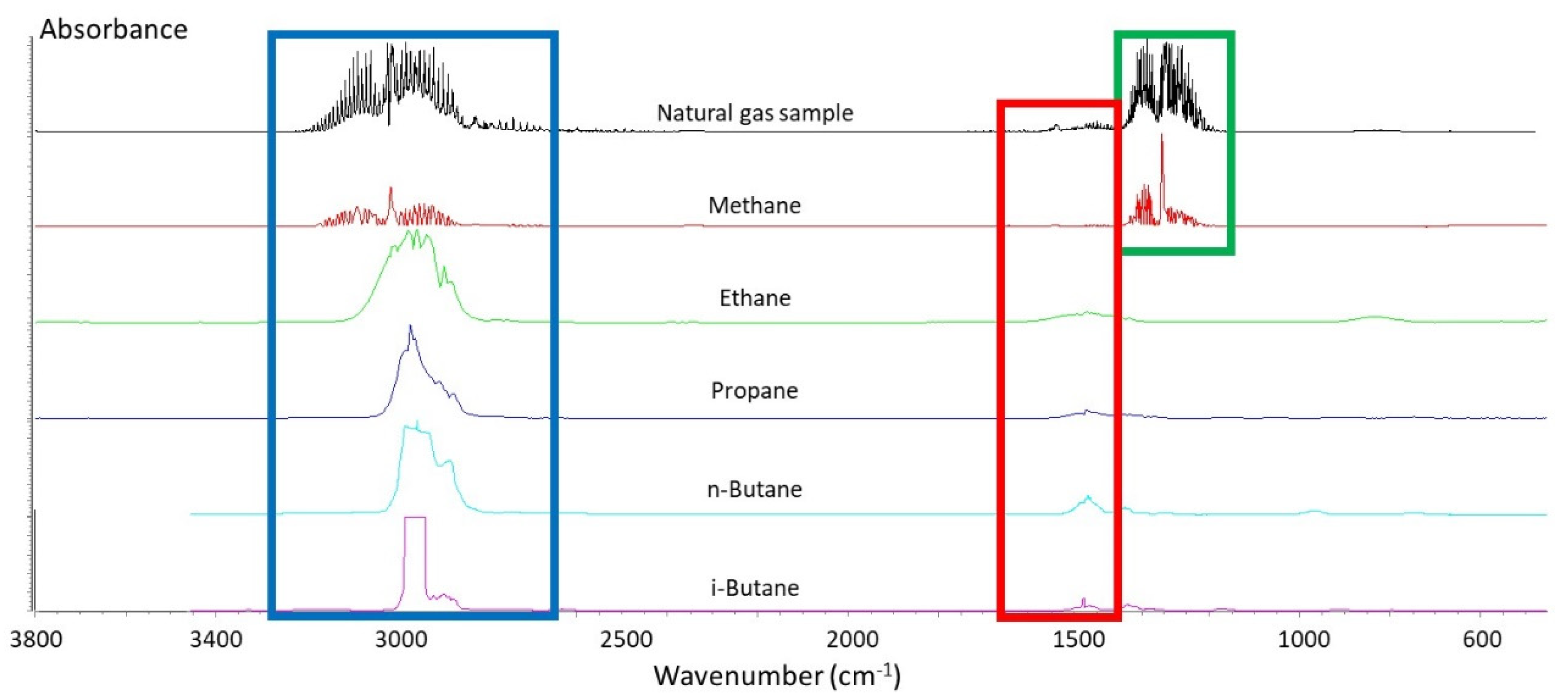
2.3. Peak Identification

Determining the components of LNG is a major issue for industries, customers, and interested parties. They are relevant to evaluate the combustion properties for its use in engines (measured experimentally by the motor methane number); for trade and energy custody activities and billing; and to evaluate the interchangeability of different gas mixtures (measured experimentally by the Wobbe index). IR spectra contain much information on the nature of the chemical constituents but, unfortunately, their spectral peaks overlap strongly because all of them have just unsubstituted hydrocarbon chains (methane, ethane, propane, butanes (i- and n-), pentanes, and, scarcely, hexane). Therefore, it is not easy to differentiate each constituent or characterize each and every compound by a unique distinctive wavenumber. Some chemical interpretation of the spectra can be obtained using reference databases, as that from NIST [39]. For example, the band at 2800–3200 cm⁻¹ (Figure 8, blue rectangle) has contributions from all the aliphatic molecules, as it corresponds to the C-H bond stretching, which is present in all components. The band at 1200–1380 cm⁻¹ (Figure 8, green rectangle) corresponds only to methane, while the band at 1380–1550 cm⁻¹ (Figure 8, red rectangle) has, again, contributions from all the other aliphatic compounds as it corresponds to the CH bending.

In the close-up image of the 1300–500 cm⁻¹ region (Figure 9), the peaks corresponding to ethane and propane can be seen. The band between 800–750 cm⁻¹ is mainly due to ethane, but for a small peak at 795 cm⁻¹ corresponding to isobutane, which is not possible to appreciate visually in the LNG spectrum. For propane, the small peaks around 750 cm⁻¹ (CH₂ and CH₃, twisting, rocking), 950–900 cm⁻¹ (CH₃, CCH deformation), and 1075–1025 cm⁻¹ (C-C, asymmetric stretching) can be seen. It is very difficult to visualize the butane peaks in the NG spectra due to its very low concentrations although, nevertheless, a small band can be ascertained at 1000–950 cm⁻¹ (corresponding to n-butane), but it could only be observed in those samples with the highest concentrations of butane (usually not exceeding 0.4%).

Table 2. Collection of the most relevant MIR spectral peaks, and their chemical assignations, for typical hydrocarbon constituents of LNG.

Methane [40]		Ethane [41]		Propane [42,43]
Description	ῦ (cm−1)	Description	ῦ (cm−1)	Description	ῦ (cm−1)	Description	ῦ (cm−1)
CH asymmetric stretch	3019	CH3 asymmetric stretch	2985	CH stretch	2957	CH3 & CH2 rocking	1186
CH symmetric stretch	2917	CH3 symmetric stretch	2895	CH stretch	2870	CH3 wagging, deformation	1155
CH symmetric bend	1543	CH3 Asymmetric deformation	1469	CH3 & CH2 scissoring	1466	C-C asymmetric stretch	1051
CH asymmetric bend	1311	CH Symmetric deformation	1379	CH3 & CH wagging (in phase)	1384	CH3 & CCH deformation	919
		CH3 rocking	821	CH3 & CH wagging (out of phase)	1368	C-C symmetric stretching	869
				CH2 & CH wagging	1331	CH2 & CH3 twisting & rocking	746
n-Butane [41]				i-Butane [44]
Description		ῦ (cm−1)		Description		ῦ (cm−1)
CH3 asymmetric stretch		2968		CH3 asymmetric stretch		2968
CH3 asymmetric stretch		2965		CH3 symmetric stretch		2956
CH3 asymmetric stretch		2912		CH3 symmetric stretch		2894
CH3 symmetric stretch		2872		CH asymmetric stretch		2872
CH2 symmetric stretch		2853		CH3 asymmetric stretch		2748
CH3 asymmetric deformation		1460		CH3 symmetric stretch		2629
CH3 scissoring		1442		CH3 asymmetric stretch		1477
CH3 twisting		1300		CH3 asymmetric bend		1379
CH3 rocking		1151		CH asymmetric bend		1334
CC stretching		1059		CCH3 bend		1177
CC stretching		837		CC stretch		925
				CC bend		797

compiles the usual positions (wavenumbers) of some relevant vibrational peaks of the constituents of a LNG sample.

2.4. Chemometric Predictive Models

The IR spectra of complex gas mixtures are too complicated to interpret by usual means. The large number of peaks and their interactions makes it almost impossible to apply simple calibration techniques and the typical Labert-Beer-Bouguer’s direct correlation is not feasible. Some of the minor components cannot be quantified directly using a specific peak, and even those with highest concentrations have a considerable number of overlapping spectral features, as seen at Figure 8 and Figure 9. Thus, considering both the full spectrum and multivariate calibration to gather relevant information is a must.

Here, the statistical and data treatment methods included in the ‘chemometrics’ field take the lead. Unfortunately, introducing the various multivariate regression methods (even only the most frequent ones) would be too lengthy, and it is out of the scope of this manuscript. Interested readers are kindly directed to some introductory texts [45,46,47,48]. It is worth citing a few important methods, namely Principal Components regression (PCR), Locally Weighted Regression (LWR), Support Vector Machines Regression (SVM(R)), or Artificial Neural Networks (ANN). Noticeably, ANNs [49] and SVM [50] were applied for quality control of natural gas, though none was applied to determine its composition. Our focus here will concentrate on the commonest, widely applied, one: PLS (partial least squares) regression, which has become a standard [2,15,51,52]. As a matter of example, PLS regression allowed the prediction of a mechanical/engine property, the methane number [53] with average prediction errors (or RMSEP) < 0.2 [16], the concentrations of ethane (error < 0.19 [16]), propane (error < 0.03 [2]), and iso and n-butane (error < 0.012 [16]), as well as the Wobbe index, a combustion property [2]. Multivariate regression models can be developed using different commercial software, such as, for instance, MATLAB’s PLS_Toolbox [54], Grams [55], Unscrambler [56], GenEx [57], SPSS [58], or Statgraphics [59], to cite some common ones. Other packages are available as freeOpen Source, e.g., CAT [60].

2.4.1. Samples

Every multivariate regression method requires a collection of samples to develop the model. In industrial environments, this can be achieved by collecting samples during a period broad enough to get a sound representation of the typical samples received/processed by the units. Different raw materials and finalized products are also welcome. This collection is then subdivided in, at least, two datasets: one for modeling and one for validating the proposed model (it is crucial to remember that the latter should always be used independently of the former). If enough samples are available, a third independent test set is advised, in order to determine the optimal number of factors. These samples have to be characterized using both the infrared procedure and the official analytical methods associated to the properties we want to predict. The absorbance of the different IR wavenumbers will act as the predictors within the models, whereas the results of the official methods will be the predictands (i.e., the values of the property to be predicted). As a rule of thumb, the proportion of samples should be around 70% for calibration, 20% for validation, and 10% for the test dataset. No doubt, it is strongly advised that all datasets represent the concentration working ranges (values of the property of interest).

2.4.2. Simplified Workflow for Model Development

In order to depict how to get a reasonable PLS model, it must be stressed from the very beginning that, although we tried to separate the workflow in individual steps for the sake of simplicity, developing a predictive regression model is an iterative and ongoing process where decisions are taken and models reformulated until a satisfactory one is obtained. This is nicely explained in public documents related to the pharmaceutical arena, where these methods are quite common today. Some of them can be of interest as introductory texts [61,62,63]. The basic steps when developing a predictive PLS model are schematized below:

• Stage 1: Preliminary assays: it is always important to visualize the spectra in order to evaluate gross differences among them, unusual signals, potential range of variables to be considered, presence of outlying samples, etc. A preliminary model can also be done to feel what its results look like and whether the samples spread through the working range of interest.
• Stage 2: spectra usually need what is called data pre-processing. This step attempts to get rid of useless information or undesired characteristics that may be detrimental for the predictions. For instance, baseline correction or noise filtering are typical steps before developing models. Very common pre-processings are the first derivative [16,64] (sometimes the 2nd derivative is also used) and mean centering [2]. Combinations of pre-processings are also common. Several options used for LNG modeling are shown in

  Table 3. Pre-processing options used by several authors before LNG multivariate modeling.

  Author	Pre-Processing
  Haghi et al. [16]	1st derivative (Savitzky–Golay algorithm), smoothing over five points plus orthogonal signal correction (OSC).
  Ferreiro et al. [2]	Iterative baseline correction (automatic weighted least squares, using a polynomial of order 2), spectral normalization (total area = 1), and mean centring.
  Barbosa et al. [4]	2nd derivative with Savitzky-Golay smoothing using 21-point windows and a 2nd order polynomial.
  Rohwedder et al. [64]	1st derivative (Savitzky–Golay algorithm) employing a 7-points window, 2nd order polynomial for baseline correction and smoothing.
  Nurida et al. [52]	Baseline correction and mean center (for CO2 absorption).

  . This stage of model development is in general recommended, although some applications argued that no pre-processing was needed [4]. There is not a definitive answer to this issue, and the unique ‘true’ advice is to try different pre-processings and see which one improves the models.
• Stage 3: A critical point to develop a satisfactory PLS model (also critical for many other techniques that use abstract factors) is to ascertain the number of factors that must be included in the model (this is called model dimensionality). Although including many factors to take account of the majority of the variance (consider variance and information as synonymous for this purpose) contained into the spectra might seem to be a good idea, it is worth considering that those factors might be unrelated to the property of interest. They might be related to baseline effects or some spurious behavior of a peak, contributing to bad predictions. Of course, we also assume that too few factors will not be sufficient to extract enough relevant information to get a sound model. So, we need to equilibrate overfitting (too many factors) with underfitting (too few factors). One of the best options for this, though not perfect, consists of performing cross-validation. This empirically evaluates a cost function so that a minimum in the error is searched for [65]. Cross-validation is iterative and sometimes takes some computer time. Its conceptual idea can be resumed in a pseudo-code as follows:
  • Fix a number of factors, let us say 1.
  • Extract, momentarily, a reduced set of samples (spectra) from the data set assigned to ‘calibration’. Several approaches can be used for this purpose, such as ‘leave-one-out’, ‘venetian blinds’, and ‘random selection of the subsets’ [66,67].
  • Develop a model, and test how well it predicts those samples left out of it. The error can be stored in the computer memory.
  • Reintegrate those spectra to the calibration set and extract another small subset of samples.
  • Develop a model, test it with the second set of left-out spectra, and sum the error to the previous one.
  • Continue the process until all samples (or possible subsets of samples) are excluded from the calibration stage and predicted afterwards. The summed errors yield the overall prediction error (=RMSECV).
  • Return to 1 and increase the number of factors by one, and repeat the process again.
  • At the end of a number of factors (for example, 20), a plot of the prediction errors will show which number of factors leads to the lowest overall prediction error (Figure 10). More details can be consulted elsewhere [65].

The procedure thus schematized is also termed ‘internal validation’, but it can still yield models that overfit the calibration set. The best way to avoid this problem is to use an external test set, if it is possible, or an external validation set (mentioned at the very beginning of this section). If the errors obtained for the internal validation (RMSECV) and the external validation (RMSEP) are similar, we can assume that the model does not overfit. That would be our best number of factors for the model (or latent variables, as it is a more correct denomination for PLS). Unfortunately, in many occasions, a clear minimum is not seen, and an inflection point where from the error do not decrease significantly has to be selected.

A nice and conceptually simple alternative to avoid overfitting without resorting to cross-validation or excluding samples consists of performing randomization. In essence, it breaks the ‘natural’ relation between spectra and their corresponding reference values (obtained after analyzing the samples with the reference methodologies), so that they are now related randomly. Then, PLS regression models that should reflect the absence of a real association between the X- and Y-variables are calculated. The randomization step is repeated a large number of times to get a sound significance, and a test statistic is calculated from all of them. Then, a critical value is derived from the distribution of those statistics. Finally, the statistic obtained for the model with the (not randomized) original data for a given number of factors is calculated. Both values are compared. A significant factor should lead to a statistic greater than the critical one. This is done successively for each factor being introduced into the model so that it is possible to decide when new factors are useless [68,69].

• Stage 4: A reason why developing a model is an iterative process is because we have to check for the existence of outlying samples. If they are present, all the previous stage is biased, and the model is not reliable. The problem is how to detect them. Likely, in the same way as you detect wrong points in a traditional calibration plot: by calculating statistics to evaluate the behavior of the samples into the model. Two of the most important and useful ones are the ‘Q residuals’ and the ‘Hotelling’s T²′ statistics [70] (another usual statistic is the leverage, although it is closely related to the T² one). The former detects whether a spectrum has some new or different spectral characteristic(s) that could not be modeled with the present model (note: ‘different’ refers to its comparison with the residuals of the other calibration spectra in the model), whereas the second evaluates how close the spectrum is to the average spectrum of the calibration set. Clearly, we would like samples with spectra close to the average and without new spectral characteristics.

From a practical viewpoint inspect graphical outputs such as, typically, the ‘Q residuals versus Hotelling’s T² plot’ and the ‘Y_residuals (predicted minus actual values for the property) versus leverage plot’. Briefly, an outlier at the former plot (a point further away from the statistical limits), such as that shown in Figure 11a (red point), will have either spectral characteristics not considered at the calibration set or much higher/lower amounts of one/several components. An outlier on the latter plot (Figure 11b) will have a high residual value, either positive or negative, which denotes that it contains more unmodeled spectral characteristics than the calibration samples do. Finally, samples deemed to be outliers should be deleted and the model reformulated (and validated) again.

• Stage 5: The external validation set of samples is of use not only to assess that the model yields no overfitting but to evaluate how good the predictions of new samples are. A typical plot, such as that in Figure 12, is of most information as it yields insight on the closeness of the individual predictions to the true values, and samples predicted badly (possible outliers?), in addition to the overall average error.

If the slope of the regression line calculated using the pairs of data in Figure 12 is statistically equal to one, both methods lead to statistically comparable results, but, for a possible background, which is given by the intercept (although it may not always hold a true significance, for instance, when large extrapolations to the zero are required). If the intercept is statistically different from zero, it indicates that there is a general offset in the predictions towards higher or lower values (when compared to the reference ones).

Furthermore, the ‘actual versus predicted’ regression line (Figure 12) is of use to calculate the procedural bias and the average precision of the multivariate model. Bias can be, simply, $\frac{\sum \left({\mathrm{x}}_{\mathrm{pred}}-{\mathrm{x}}_{\mathrm{true}}\right)}{\mathrm{m}}$, (m = number of samples). Repeatability precision can be evaluated quite easily as the standard error of the regression line (s_y/x), just assuming that the error in the reference values is negligible in comparison to the PLS predictions [65,71]. That is true when using standardized chromatographic methodologies but not so evident when complex methods, such as the motor methane number, are used. Reproducibility precision can be roughly the average prediction error, calculated as $\mathrm{RMSEP}=(\sqrt{\frac{\sum {\left({\mathrm{x}}_{\mathrm{pred}}-{\mathrm{x}}_{\mathrm{true}}\right)}^2}{\mathrm{m}}})$, m = number of validation samples, and ‘pred’ stands for predicted. This term can be bias-corrected considering RMSEP_corrected = RMSEP − bias (if bias is zero, the usual statement that RMSEP is the reproducibility precision holds fine).

It is also worth noting that Figure 12 can be used to calculate figures or merit related to the modern limits of detection (where the risks of false positives and false negatives are controlled [72,73,74,75,76]) and to derive a sample-specific confidence interval associated to each prediction. Calculations for the former topic are not trivial, and readers are kindly forwarded to the references given above. As a snapshot, the classical, old (1970s decade) limit of detection is today termed critical limit, and it only takes account for the risk of false positives. It can be estimated as x_c = (t_(α,N-2)·w₀·s_y/x)/b, with t = one-tail Student’s statistic, and w₀·s_y/x = standard error at zero concentration derived from the ‘predicted versus actual’ regression; b is the slope [72,74]. The ‘limit of detection’ (indeed, this term has been superseded, and it should be now called capability of detection or minimum detectable net concentration) has a very similar equation, although using a non-central t distribution instead of the current Student’s one in order to consider the risks of false positives and false negatives simultaneously (both at 95% confidence level).

With regard to the second topic, in simple terms, the sample-specific confidence interval can be formulated as [predicted value ± t·S_xo], where t is the Student’s t value for ν degrees of freedom at a 95% confidence level. S_xo is the specific standard error of the prediction [77,78], which can be estimated as ${\left[\left(1+{\mathrm{h}}_i\right)·{\mathrm{RMSEC}}^2-{\mathrm{S}}_{ref}^2·\left(\raisebox{1ex}{$\mathsf{\nu }$}\!\left/ \!\raisebox{-1ex}{${\mathrm{X}}^2$}\right.\right)\right]}^{1/2}$, where h_i is the leverage for sample i, RMSEC is the standard error of the calibration, S_ref is the measurement error in the reference value, and X² is the X² statistic (ν degrees of freedom and 95% confidence level) used to avoid overcorrection of the bias term [79]. The fact that the equation includes the leverage of the sample (which depends on its position in the factorial space of the model) particularizes the equation for each sample. Hence, the denomination sample-specific as it calculates a different confidence interval for each sample. Note also that it takes account of the error in the reference values.

3. Conclusions

The new analytical methodology proposed in this work for routine LNG quality control is composed of two major steps: infrared spectral measurement of a gaseous sample and chemometric model development. It was reviewed that the most important parameters that affect the measurements are the instrument (spectral range, operational characteristics, such as resolution, number of scans, apodization, and background collection) and the gas cell (pathlength, internal pressure, broadening gas, windows). The tiered development of a chemometric model was reviewed, and it was found to be composed of several intertwined steps: pre-processing, outlier detection, regression method, cross-validation, and validation.

The combination of the spectrometric and chemometric methods has some interesting advantages for routine quality control: high speed, reduced costs, reduced use of reagents, and high flexibility (as the same spectrum can be used to predict several LNG properties). Hence, the hybridization of FTIR and multivariate regression (in particular, PLS) yields a reliable, powerful alternative to the traditional, standardized Gas Chromatography approach for routine measurements.

References

1. ISO 6974-1: 2013 Natural Gas—Determination of Composition and Associated Uncertainty by Gas Chromatography—Part 1: General Guidelines and Calculation of Composition; ISO: Geneva, Switzerland, 2013.
2. Ferreiro, B.; Andrade, J.; López-Mahía, P.; Muniategui, S.; Vázquez, C.; Pérez, A.; Rey, M.; Vales, C. Fast quality control of natural gas for commercial supply and transport utilities. Fuel 2021, 305, 121500. [Google Scholar] [CrossRef]
3. Kiefer, J. Recent advances in the characterization of gaseous and liquid fuels by vibrational spectroscopy. Energies 2015, 8, 3165–3197. [Google Scholar] [CrossRef] [Green Version]
4. Barbosa, M.F.; Santos, J.R.B.; Silva, A.N.; Soares, S.F.C.; Araujo, M.C.U. A cheap handheld NIR spectrometric system for automatic determination of methane, ethane, and propane in natural gas and biogas. Microchem. J. 2021, 170, 106752. [Google Scholar] [CrossRef]
5. Koturbash, T.; Karpash, M.; Darvai, I.; Rybitskyi, I.; Kutcherov, V. Development of new instant technology of natural gas quality determination. In Proceedings of the ASME 2013 Power Conference, Boston, MA, USA, 29 July–1 August 2013; Volume 1. [Google Scholar] [CrossRef] [Green Version]
6. Looney, B. Statistical Review of World Energy 2021. Rev. World Energy Data 2021, 70, 8–20. [Google Scholar]
7. Hosseini, M.; Dincer, I.; Ozbilen, A. Expert Opinions on Natural Gas Vehicles Research Needs for Energy Policy Development; Elsevier: Amsterdam, The Netherlands, 2018; ISBN 9780128137352. [Google Scholar]
8. BP, P.L.C. Natural Gas Demand. Available online: https://www.bp.com/en/global/corporate/energy-economics/energy-outlook/demand-by-fuel/natural-gas.html (accessed on 20 October 2021).
9. Rahmouni, C.; Tazeroutb, M.; Le-Corre, O. Determination of the combustion properties of natural gases by pseudo-constituents. Fuel 2003, 82, 1399–1409. [Google Scholar] [CrossRef]
10. Roy, P.S.; Ryu, C.; Park, C.S. Predicting Wobbe Index and methane number of a renewable natural gas by the measurement of simple physical properties. Fuel 2018, 224, 121–127. [Google Scholar] [CrossRef]
11. Karpash, O.; Darvay, I.; Karpash, M. New approach to natural gas quality determination. J. Pet. Sci. Eng. 2010, 71, 133–137. [Google Scholar] [CrossRef]
12. Sweelssen, J.; Blokland, H.; Rajamäki, T.; Boersma, A. Capacitive and Infrared Gas Sensors for the Assessment of the Methane Number of LNG Fuels. Sensors 2020, 20, 3345. [Google Scholar] [CrossRef]
13. Sweelssen, J.; Blokland, H.; Rajamäki, T.; Sarjonen, R.; Boersma, A. A versatile capacitive sensing platform for the assessment of the composition in gas mixtures. Micromachines 2020, 11, 116. [Google Scholar] [CrossRef] [Green Version]
14. Boersma, A.; Sweelsen, J.; Blokland, H. Gas Composition Sensor for Natural Gas and Biogas. Procedia Eng. 2016, 168, 197–200. [Google Scholar] [CrossRef]
15. Makhoukhi, N.; Péré, E.; Creff, R.; Pouchan, C. Determination of the composition of a mixture of gases by infrared analysis and chemometric methods. J. Mol. Struct. 2005, 744–747, 855–859. [Google Scholar] [CrossRef]
16. Haghi, R.K.; Yang, J.; Tohidi, B. Fourier Transform Near-Infrared (FTNIR) Spectroscopy and Partial Least-Squares (PLS) Algorithm for Monitoring Compositional Changes in Hydrocarbon Gases under In Situ Pressure. Energy Fuels 2017, 31, 10245–10259. [Google Scholar] [CrossRef]
17. Ribessi, R.L.; Neves, T.D.A.; Rohwedder, J.J.R.; Pasquini, C.; Raimundo, I.M.; Wilk, A.; Kokoric, V.; Mizaikoff, B. IHEART: A miniaturized near-infrared in-line gas sensor using heart-shaped substrate-integrated hollow waveguides. Analyst 2016, 141, 5298–5303. [Google Scholar] [CrossRef] [Green Version]
18. Dąbrowski, K.M.; Kuczyński, S.; Barbacki, J.; Włodek, T.; Smulski, R.; Nagy, S. Downhole measurements and determination of natural gas composition using Raman spectroscopy. J. Nat. Gas Sci. Eng. 2019, 65, 25–31. [Google Scholar] [CrossRef]
19. Eichmann, S.C.; Kiefer, J.; Benz, J.; Kempf, T.; Leipertz, A.; Seeger, T. Determination of gas composition in a biogas plant using a Raman-based sensorsystem. Meas. Sci. Technol. 2014, 25, 075503. [Google Scholar] [CrossRef]
20. Sieburg, A.; Knebl, A.; Jacob, J.M.; Frosch, T. Characterization of fuel gases with fiber-enhanced Raman spectroscopy. Anal. Bioanal. Chem. 2019, 411, 7399–7408. [Google Scholar] [CrossRef]
21. Specac Product Catalogue. Available online: https://www.specac.com/en/documents/catalogues (accessed on 25 November 2021).
22. Microptik Gas Sampling. Available online: https://www.microptik.eu/product/gas-sampling (accessed on 25 November 2021).
23. Jasco Gas Cells. Available online: https://jascoinc.com/products/spectroscopy/ftir-spectrometers/ftir-accessories/gas-cells/ (accessed on 25 November 2021).
24. Guiding Photonics Gas Cells. Available online: https://guidingphotonics.com/gas-cells/ (accessed on 21 September 2021).
25. Kriesel, J.M.; Gat, N.; Bernacki, B.E.; Erikson, R.L.; Cannon, B.D.; Myers, T.L.; Bledt, C.M.; Harrington, J.A. Hollow core fiber optics for mid-wave and long-wave infrared spectroscopy. In Proceedings of the International Society for Optics and Photonics, Orlando, FL, USA, 26–28 April 2011; Volume 8018, p. 80180V. [Google Scholar]
26. Li, N.; Tao, L.; Yi, H.; Kim, C.S.; Kim, M.; Canedy, C.L.; Merritt, C.D.; Bewley, W.W.; Vurgaftman, I.; Meyer, J.R. Methane detection using an interband-cascade LED coupled to a hollow-core fiber. Opt. Express 2021, 29, 7221–7231. [Google Scholar] [CrossRef]
27. Pike Technologies. Choice of Window Materials for Transmission Sampling of Liquids in the Mid-IR Spectral Region. Available online: https://www.piketech.com/skin/fashion_mosaic_blue/application-pdfs/CrystalChoiceForTransmission.pdf (accessed on 25 November 2021).
28. Shimadzu Corporation Safety of Windows and Prisms Used in FTIR. Available online: https://www.shimadzu.com/an/service-support/technical-support/analysis-basics/tips-ftir/safety.html (accessed on 20 September 2021).
29. Spectra-Tech. How to Select an Infrared Transmission Window 2012. Available online: https://kinecat.pl/wp-content/uploads/2012/11/crystal_ref.pdf (accessed on 25 November 2021).
30. Smith, B.C. Fundamentals of Fourier Transform Infrared Spectroscopy, 1st ed.; CRC Press: Boca Raton, FL, USA, 2011; ISBN 1420069306. [Google Scholar]
31. Griffiths, P.R.; De Haseth, J.A. Fourier Transform Infrared Spectrometry; John Wiley & Sons: Chichester, UK, 2007; Volume 171, ISBN 0470106298. [Google Scholar]
32. Harris, D.C. Análisis Químico Cuantitativo; Reverté: Barcelona, Spain, 2007; ISBN 8429172246. [Google Scholar]
33. Skoog, D.A.; Holler, F.J.; Nieman, T.A. Principios de Análisis Instrumental, 7th ed.; Cengage Learning: Boston, MA, USA, 2018; ISBN 978-607-481-390-6. [Google Scholar]
34. Stuart, B. Infrared Spectroscopy. In Kirk-Othmer Encyclopedia of Chemical Technology, 1st ed.; John Wiley & Sons: Chichester, UK, 2015; pp. 73–101. ISBN 0471238961. [Google Scholar]
35. Anderson, P.W. Pressure Broadening in the Microwave and Infra-Red Regions. Phys. Rev. 1949, 76, 647–661. [Google Scholar] [CrossRef]
36. Jabloński, A. General Theory of Pressure Broadening of Spectral Lines. Phys. Rev. 1945, 68, 78–93. [Google Scholar] [CrossRef]
37. Margenau, H.; Watson, W.W. Pressure effects of foreign gases on the sodium D-lines. Phys. Rev. 1933, 44, 92–98. [Google Scholar] [CrossRef]
38. Ferreiro, B.; Andrade, J.M.; Paz-Quintáns, C.; López-Mahía, P.; Muniategui-Lorenzo, S.; Rey-Garrote, M.; Vázquez-Padín, C.; Vales, C. Improved Sensitivity of Natural Gas Infrared Measurements Using a Filling Gas. Energy Fuels 2019, 33, 6929–6933. [Google Scholar] [CrossRef]
39. NIST Public. IR Spectra Database. Available online: https://webbook.nist.gov/chemistry/name-ser/ (accessed on 25 November 2021).
40. Es-Sebar, E.; Farooq, A. Intensities, broadening and narrowing parameters in the ν3 band of methane. J. Quant. Spectrosc. Radiat. Transf. 2014, 149, 241–252. [Google Scholar] [CrossRef] [Green Version]
41. Shimanouchi, T. Tables of Molecular Vibrational Frequencies: Part 6. J. Phys. Chem. Ref. Data 1973, 2, 121–162. [Google Scholar] [CrossRef]
42. Gough, K.M.; Murphy, W.F.; Raghavachari, K. The harmonic force field of propane. J. Chem. Phys. 1987, 87, 3332–3340. [Google Scholar] [CrossRef]
43. Hudson, R.L.; Gerakines, P.A.; Yarnall, Y.Y.; Coones, R.T. Infrared spectra and optical constants of astronomical ices: III. Propane, propylene, and propyne. Icarus 2021, 354, 114033. [Google Scholar] [CrossRef]
44. Evans, J.C.; Bernstein, H.J. The vibrational spectra of isobutane and isobutane-d1. Can. J. Chem. 1956, 34, 1037–1045. [Google Scholar] [CrossRef]
45. Brereton, R.G. Chemometrics: Data Analysis for the Laboratory and Chemical Plant; John Wiley & Sons: Chichester, UK, 2003; ISBN 0470845740. [Google Scholar]
46. Otto, M. Chemometrics: Statistics and Computer Application in Analytical Chemistry; John Wiley & Sons: Chichester, UK, 2016; ISBN 3527340971. [Google Scholar]
47. Wold, S.; Esbensen, K.; Geladi, P. Principal component analysis. Chemom. Intell. Lab. Syst. 1987, 2, 37–52. [Google Scholar] [CrossRef]
48. Martens, H. Reliable and relevant modelling of real world data: A personal account of the development of PLS Regression. Chemom. Intell. Lab. Syst. 2001, 58, 85–95. [Google Scholar] [CrossRef]
49. Gupta, S.K.; Mittal, M. Predicting the methane number of gaseous fuels using an artificial neural network. Biofuels 2019, 12, 1191–1198. [Google Scholar] [CrossRef]
50. Bai, P.; Duan, X.; He, C.; Li, Y. Natural gas infrared spectrum analysis based on multi-level and SVM-subset. In Proceedings of the 2009 IEEE International Conference on Virtual Environments, Human-Computer Interfaces and Measurements Systems, Hong Kong, 11–13 May 2009; IEEE: Piscataway, NJ, USA, 2009; pp. 336–339. [Google Scholar]
51. Udina, S.; Carmona, M.; Pardo, A.; Calaza, C.; Santander, J.; Fonseca, L.; Marco, S. A micromachined thermoelectric sensor for natural gas analysis: Multivariate calibration results. Sens. Actuators B Chem. 2012, 166–167, 338–348. [Google Scholar] [CrossRef]
52. Nurida, M.Y.; Norfadilah, D.; Aishah, M.R.S.; Phak, C.Z.; Saleh, S.M. Monitoring of CO2 Absorption Solvent in Natural Gas Process Using Fourier Transform Near-Infrared Spectrometry. Int. J. Anal. Chem. 2020, 2020, 1–9. [Google Scholar] [CrossRef] [Green Version]
53. Ponte, S.; Andrade, J.M.; Vázquez, C.; Ferreiro, B.; Cobas, C.; Pérez, A.; Rey, M.; Vales, C.; Pellitero, J.; Santacruz, B.; et al. Prediction of the methane number of commercial liquefied natural gas samples using mid-IR gas spectrometry and PLS regression. J. Nat. Gas Sci. Eng. 2021, 90, 103944. [Google Scholar] [CrossRef]
54. Wise, B.M.; Gallagher, N.B.; Bro, R.; Shaver, J.; Windig, W.; Koch, J. PLS_Toolbox; Eigenvector Research Inc.: Manson, WA, USA, 2006. [Google Scholar]
55. ThermoFisher Scientific. Available online: https://www.thermofisher.com/order/catalog/product/INF-15004 (accessed on 25 November 2021).
56. Aspen Technology Inc. Unscrambler. Available online: https://www.aspentech.com/en/products/msc/aspen-unscrambler (accessed on 24 November 2021).
57. MultiD Analyses, B.D. Genex. Available online: https://multid.se/genex/ (accessed on 24 November 2021).
58. IBM Co. IBM SPSS Software. Available online: https://www.ibm.com/es-es/analytics/spss-statistics-software (accessed on 24 November 2021).
59. Statgraphics Technologies, Inc. Available online: https://www.statgraphics.com/ (accessed on 24 November 2021).
60. Leardi, R.; Melzi, C.; Polotti, G. CAT (Chemometric Agile Tool), Freely. Available online: http://gruppochemiometria.it/index.php/software (accessed on 4 November 2021).
61. Broad, N.; Graham, P.; Hailey, P.; Hardy, A.; Holland, S.; Hughes, S.; Lee, D.; Prebble, K.; Salton, N.; Warren, P. Guidelines for the Development and Validation of Near-Infrared Spectroscopic Methods in the Pharmaceutical Industry. In Handbook of Vibrational Spectroscopy; John Wiley & Sons: Chichester, UK, 2002; Volume 5, pp. 3590–3610. [Google Scholar]
62. Validation of Analytical Procedures: Text and Methodology. In ICH Harmonised Tripartite Guideline; Somatek Inc.: San Diego, CA, USA, 2014.
63. European Medicines Agency Guideline on the Use of Near Infrared Spectroscopy (NIRS) by the Pharmaceutical Industry and the Data Requirements for New Submissions and Variations. 2012. Available online: https://www.ema.europa.eu/en/use-near-infrared-spectroscopy-nirs-pharmaceutical-industry-data-requirements-new-submissions (accessed on 25 November 2021).
64. Rohwedder, J.J.R.; Pasquini, C.; Fortes, P.R.; Raimundo, I.M.; Wilk, A.; Mizaikoff, B. iHWG-μNIR: A miniaturised near-infrared gas sensor based on substrate-integrated hollow waveguides coupled to a micro-NIR-spectrophotometer. Analyst 2014, 139, 3572. [Google Scholar] [CrossRef] [Green Version]
65. Andrade-Garda, J.M.; Carlosena-Zubieta, A.; Boqué-Martí, R.; Ferré-Baldrich, J. Partial Least Squares Regression. In Basic Chemometric Techniques in Atomic Spectroscopy; Andrade-Garda, J.M., Ed.; Royal Society of Chemistry: Cambridge, UK, 2013; pp. 280–347. ISBN 1849737967. [Google Scholar]
66. Malinowski, E.R.; Howery, D.G. Factor Analysis in Chemistry; Wiley: Hoboken, NJ, USA, 1980; ISBN 0471058815. [Google Scholar]
67. Eigenvector Research Eigenvector Wiki. Available online: https://www.wiki.eigenvector.com/index.php?title=Confusionmatrix (accessed on 14 May 2021).
68. Faber, N.M.; Rajkó, R. How to avoid over-fitting in multivariate calibration-The conventional validation approach and an alternative. Anal. Chim. Acta 2007, 595, 98–106. [Google Scholar] [CrossRef]
69. Wiklund, S.; Nilsson, D.; Eriksson, L.; Sjöström, M.; Wold, S.; Faber, K. A randomization test for PLS component selection. J. Chemom. 2007, 21, 427–439. [Google Scholar] [CrossRef]
70. Vinzi, V.E.; Chin, W.W.; Henseler, J.; Wang, H. Handbook of Partial Least Squares; Springer: Berlin/Heidelberg, Germany, 2010; ISBN 978-3-540-32825-4. [Google Scholar]
71. Sanz, M.B.; Sarabia, L.A.; Herrero, A.; Ortiz, M.C. Multivariate analytical sensitivity in the determination of selenium, copper, lead and cadmium by stripping voltammetry when using soft calibration. Anal. Chim. Acta 2003, 489, 85–94. [Google Scholar] [CrossRef]
72. Ortiz, M.C.; Sarabia, L.A.; Sánchez, M.S. Tutorial on evaluation of type I and type II errors in chemical analyses: From the analytical detection to authentication of products and process control. Anal. Chim. Acta 2010, 674, 123–142. [Google Scholar] [CrossRef]
73. Ortiz, M.C.; Sarabia, L.A.; Herrero, A.; Sánchez, M.S.; Sanz, M.B.; Rueda, M.E.; Giménez, D.; Meléndez, M.E. Capability of detection of an analytical method evaluating false positive and false negative (ISO 11843) with partial least squares. Chemom. Intell. Lab. Syst. 2003, 69, 21–33. [Google Scholar] [CrossRef]
74. ISO 11843. Capability of Detection–Part 2: Methodology in the Linear Calibration Case; ISO: Geneva, Switzerland, 2008. [Google Scholar]
75. SANCO/2004/2726 Guidelines for the Implementation of Decision 2002/657/EC. Rev 4-December 2008. Available online: https://ec.europa.eu/food/system/files/2016-10/cs_vet-med-residues_cons_2004-2726rev4_en.pdf (accessed on 25 November 2021).
76. European Commission. Commission Decision 2002/657/EC of 12 August 2002 implementing Council Directive 96/23/EC concerning the performance of analytical methods and the interpretation of results. Off. J. Eur. Communities 2002, 50, 8–36. [Google Scholar]
77. Faber, K.; Kowalski, B.R. Prediction error in least squares regression: Further critique on the deviation used in The Unscrambler. Chemom. Intell. Lab. Syst. 1996, 34, 283–292. [Google Scholar] [CrossRef]
78. Faber, N.M.; Schreutelkamp, F.H.; Vedder, H.W. Estimation of prediction uncertainty for a multivariate calibration model. Spectrosc. Eur. 2004, 16, 17–21. [Google Scholar]
79. Faber, K.; Kowalski, B.R. Improved prediction error estimates for multivariate calibration by correcting for the measurement error in the reference values. Appl. Spectrosc. 1997, 51, 660–665. [Google Scholar] [CrossRef]
Figure 1. Basic diagram of a hollow-core fiber cell internal structure. Source: guidingphotonics.com (accessed on 20 November 2021) [24].
Energies 15 00359 g001
Figure 2. Comparison of spectra obtained using a multireflection gas cell (1 m pathlength) with CaF2 windows (yellow) and a single-pass gas cell (10 cm) with ZnSe windows. The region in the box shows the influence of the windows (see text for details).
Energies 15 00359 g002
Figure 3. Conceptual scheme of the 10 cm-path gas cell tailored for measuring regasified LNG samples.
Energies 15 00359 g003
Figure 4. Instrumental setup with a gas cylinder connected to the 3-way valve so that the sample and the broadening gas can be introduced into the cell.
Energies 15 00359 g004
Figure 5. Effect of the nominal resolution on the IR natural gas spectra. Black: 1 cm−1; Red: 8 cm−1 resolution.
Energies 15 00359 g005
Figure 6. Baseline evolution of the spectrum of a sample during 1 h without background correction.
Energies 15 00359 g006
Figure 7. Exemplification of the effect of a broadening gas (Ar) on the intensity of a weak peak of an LNG sample (named B4X) at 1716 cm−1 (attributed to CH bending). The inset shows the ratio of variation of the signal as a function of the pressure of Ar. The pressure of the sample was always 0.2 bar, whereas the total pressure is indicated in the labels.
Energies 15 00359 g007
Figure 8. Comparison between the spectra of regasified LNG and its main aliphatic components (as stated in Reference [39]).
Energies 15 00359 g008
Figure 9. Close-up view of the 1300–500 cm−1 (a) and 1600–1340 cm−1 (b) regions of a LNG spectrum (depicted in Figure 8).
Energies 15 00359 g009
Figure 10. Examples of RMSEC-RMSECV plots for decision-making. The best number of factors (Latent Variables) is indicated with an arrow. Note that the RMSEC (root mean square error in calibration) diminishes monotonically; so it is useless to select the dimensionality of the models. RMSECV stands for root mean square error in cross-validation.
Energies 15 00359 g010
Figure 11. (a) Hotelling’s T2 versus Q residuals plot and (b) Y_residuals versus leverage plot. One of the outlying samples is shown in red.
Energies 15 00359 g011
Figure 12. Typical comparison between the PLS-predicted values and the reference or ‘true’ ones. See text for the different studies that can be derived from it.
Energies 15 00359 g012