Operation Characteristics of Adjustable Field IPMSM Utilizing Magnetic Saturation

Abstract

This paper describes an interior permanent magnet synchronous motor (IPMSM) based on a new adjustable field method. The proposed PM motor achieved magnetic field control utilizing magnetic saturation. In this paper, a back electromotive force (e.m.f.) measurement test and a load test using the prototype motor were conducted to clarify if the proposed motor had a wide operation range. In the back e.m.f. measurement test, it was confirmed that the proposed motor had a wide magnetic field controllable range of 51.7%. In addition, it was revealed, through the load test, that the proposed motor had a wide operating range, including both low-speed high-torque and high-speed low-torque driving conditions. Moreover, based on electromagnetic field analysis, the magnetic field control performance of the proposed adjustable field method was compared with the conventional field weakening control and other adjustable field methods. As a comparison result, it was verified that the proposed motor had less copper loss for the magnetic field control and fewer losses in the high-speed operating range.

1. Introduction

Since the Paris agreement was signed in 2015, countries around the world have been working intensively to save energy. Particularly, in the electric machine technical field, the high-efficiency motor has actively been researched. A permanent magnet synchronous motor (PMSM) using high-power density permanent magnets (PMs) has widely been used because the PMSM can make the high-efficiency and high-power density drive possible [1,2]. In addition to the efficiency and the power density, a wide driving range is one of the most important evaluation items of the motor used in automotive applications. Generally, a design that achieves both low-speed high-torque and high-speed low-torque operations is required. However, it is challenging to achieve these operations at the same time because the magnetic field of the PMSM is not adjustable. Conventionally, field weakening control has been applied to expand the high-speed operation range [3,4]. The field weakening control has traditionally employed and can undermine the magnetic field of the PMSM by using the negative d-axis current i_d. However, there is a problem whereby the copper loss increase in the high-speed operation range is not ignorable, because the field weakening control requires much current to give a counter magnetic field against the PM field. To make matters worse, the counter magnetic field generated by the negative i_d may cause irreversible demagnetization of PMs in the rotor.

To solve this problem, in previous studies, an adjustable field PMSM that can control the PM-based magnetic field has been attracting attention in recent years [5,6,7,8,9,10,11]. The adjustable field PMSM introduced in the references [5,6] can control the magnetic field density on the rotor surface with a consequent pole structure by using a field winding. However, it has low torque density as implemented in surface permanent magnet synchronous motor (SPMSM) configuration. As known well among the researchers, the SPM configuration does not have capability to generate a reluctance torque additional to the magnet torque. The PMs of the adjustable field SPMSM can easily demagnetize due to the long air gap length. In the reference [7], the magnetic field passing through the magnetic leakage path on the rotor core is controlled by q-axis magnetomotive force (m.m.f.). This adjustable field method can realize the magnetic field control with a single inverter, because the additional m.m.f. source is not required. As a result, the magnetic field is dependent on motor operation. The adjustable field principle utilizing the motor harmonics is described in the reference [8]. This method uses the 2nd order space harmonics generated by the concentrated winding structure for the magnetic field control. However, this method cannot control the magnetic field actively and arbitrarily, because the rotating speed governs the quantity of the magnetic field. Furthermore, this motor must use soft magnetic composite (SMC) material, which is difficult to produce.

The adjustable field method proposed in the reference [9] can make an expansive driving range possible, because this method can change the drive circuits that correspond to three-phase or six-phase windings, etc. However, multiple six single-phase inverters are indispensable to switch over the winding configurations. For this reason, there is a drawback that the drive system of this adjustable field PMSM can be larger than other conventional motors. Furthermore, this method has only four discrete magnetic field outputs, resulting in a discrete adjustment of the magnetic field. The IPMSM utilizing the de- and re-magnetization of the PMs can achieve wide-range control of the magnetic field and highly efficient drive [10,11]. However, the drive system for the adjustable field IPMSM based on this approach tends to be bulky, because an extremely high m.m.f. is indispensable for de- and re-magnetization. In general, several significant problems in existing adjustable field methods are the motor type, which cannot deliver the reluctance torque; detrimental influence on the motor operation and rotating speed; demagnetization of PMs; magnetic field controllability; difficulty in manufacturing; and high copper loss for magnetic field control.

The authors have been investigating a new adjustable field method focusing on the magnetic saturation of the magnetic material [12]. The magnetic saturation is a phenomenon in which magnetic permeability changes according to the intensity of the external magnetic field. Typically, this phenomenon detrimentally affects the performance of the motor output in conventional motor drives [13,14]. In the reference [13], it was confirmed, through the analysis, that d- and q-axis flux linkage and torque are affected by the magnetic saturation. In another reference about the influence of the magnetic saturation [14], the relationship between the rotor bridge and the performance of a spoke-type PMSM was mathematically derived. In addition, it was revealed that the magnetic saturation in the bridge part has a significant influence on the motor performance. As mentioned above, the magnetic saturation usually deteriorates the motor output and complicates the design and the control.

As a novelty, the authors propose a motor with an adjustable field method utilizing the magnetic saturation (the proposed motor) in this paper to overcome disadvantages of the conventional field weakening control and the previous adjustable field methods. Detailed contributions of this paper are as follows:

(1)

Adjustable field capability with genuine electromagnetic operation;

(2)

Capability of the reluctance torque generation;

(3)

Independency of the field adjustment on the motor operation (vector control) and the rotating speed;

(4)

Higher anti-demagnetization capability of PMs;

(5)

Continuous magnetic field control;

(6)

Better productivity of the motor hardware;

(7)

Lower copper loss for magnetic field control.

Finally, the proposed motor had a wider controllable range of the magnetic field by 51.7%.

In the following section, the principle of the proposed adjustable field method is introduced and explained in detail. Back e.m.f. characteristics are explained in Section 3. The drive system of the prototype motor and its load characteristic test results are described in Section 4 and Section 5, respectively. Finally, the paper concludes in Section 6 with some highlights of the research study.

2. Principle of Adjustable Field Method Utilizing Magnetic Saturation

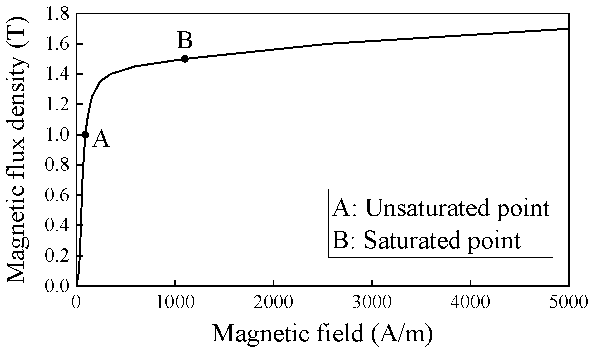
As mentioned above, the proposed adjustable field method uses magnetic saturation of the magnetic material. Figure 1 shows the relationship between the magnetic flux density and the magnetic field (B–H curve) of 35JNE230, used for the prototype motor’s core. The permeability is defined as a slope of the B–H characteristic. As shown in Figure 1, the permeability of the core changes depending on the external magnetic field.

The magnetic circuit and specifications of the prototype motor are shown in Figure 2 and

Table 1. Specifications of prototype motor.

Parameter	Value
Number of poles and slots	8 poles, 48 slots
Armature winding	6 turns/slot, 0.15 Ω
Modulation winding	120 turns, 1.8 Ω
Stator diameter	ϕ148 mm
Rotor diameter	ϕ96.6 mm
Stack length	63 mm

, respectively. As shown in Figure 2, the prototype motor was an IPMSM. Therefore, the prototype motor could deliver the reluctance torque. The stator and rotor cores of the prototype motor were split into two parts and an additional winding was inserted between the split stator cores. The additional winding generated a magnetic flux to cause magnetic saturation and to control the magnetic field. There were magnetic leakage paths between PMs in the rotor core in the prototype motor. The magnetic flux modulated the permeability of the magnetic leakage paths. Therefore, the additional winding and the magnetic flux were called modulation winding and modulation flux, respectively. The resistance of the modulation winding was larger than that of the armature winding. The voltage drop and inductance became large by designing the modulation winding with a large resistance value. However, the voltage drop was negligibly small compared to the phase voltage and DC-bus voltage, so the effect was small. In addition, there was no effect of the large inductance because the DC modulation current was used. S45C, a carbon steel material, was used as the rotor shaft and the stator frame to penetrate the modulation flux in the 3-dimensional (3D) magnetic path. Generally, the iron loss in the 3D magnetic path was reduced by constructing the 3D path with an SMC [15,16]. However, it costs a lot to make the SMC core, because high pressure around 1000 MPa is indispensable [17]. On the other hand, the proposed IPMSM could use a steel material as the 3D magnetic path because the modulation flux included only a DC or low-frequency component. For this reason, the 3D magnetic path could easily be realized.

Figure 3 shows a vector plot of the modulation flux when the m.m.f. F_m used for magnetic field control was given to the modulation winding. In this paper, all analysis results were obtained from the FEM using JMAG-Designer. As shown in Figure 3a, the modulation flux penetrated in the radial direction. There was a leakage flux passing through the air between the two stator cores, as shown in Figure 3b. However, the amount of the leakage flux was negligibly small because the air gap between the two stator cores was 15 mm, which is much larger than the air gap length between the stator core and the rotor core. In addition, the rotor shaft and the stator frame were magnetized by the DC modulation flux, but the residual flux was negligibly small because S45C, which is a soft magnetic material, was used as the material for the rotor shaft and the stator frame.

It was confirmed, from Figure 3, that the modulation flux penetrated in the radial direction. In the stator, no iron loss occurred because the modulation flux was DC flux. In addition, there was also no iron loss in the rotor due to the modulation flux. Figure 4 was prepared to examine why iron loss did not occur in the rotor. Figure 4a shows a usual DC flux and Figure 4b shows a radial DC flux similar to the modulation flux. As shown in Figure 4a, the observation point in front of the N-pole magnet was defined and the change in magnetic flux in the observation point was verified. Figure 5 shows the magnetic flux fluctuations of the d- and the q-axis components. Usually, as can be seen in Figure 5a, when the magnetic flux was transmitting, the magnetic flux component in the rotor fluctuated due to the rotation of the rotor, even if the magnetic flux was DC. On the other hand, as can be seen in Figure 5b, when the magnetic flux penetrated in all radial directions, there was no variation in the magnetic flux with respect to time. From the above results, it can be inferred that there was no effect on iron loss when the DC modulation flux was used for the adjustable field.

Figure 6 shows vector plots of the PM flux and the modulation flux with an F_m of 0 AT, 720 AT and 1200 AT. Without the F_m, many PM fluxes leaked in the rotor core. In this case, the permeability of both the N- and S-pole side magnetic leakage path was 50. With an F_m of 720 AT, the permeability of the N-pole side magnetic leakage path decreased to 24 by the modulation flux. Therefore, it became difficult for the N-pole PM flux to leak through the magnetic leakage path and the N-pole PM flux interlinking to the stator core increased. However, since the modulation flux penetrated in the direction weakening the N-pole magnet, it was necessary to study the de-magnetization of the N-pole PM. On the other hand, the permeability of the S-pole side magnetic leakage path increased to 3000 by the modulation flux. In this case, many modulation fluxes penetrated through the S-pole side magnetic leakage path and strengthened the magnetic field of the S-pole. With an F_m of 1200 AT, the magnetic field of the proposed motor reached its limit, because the permeability of both the N- and S-pole side magnetic leakage paths decreased and the modulation flux could no longer penetrate. In this way, the proposed motor can realize magnetic field control by using magnetic saturation and modulating the permeability of the magnetic leakage paths.

Figure 7 shows the magnetic flux density in the air gap between the upper stator core and rotor core with an F_m of 0 AT, 720 AT and 1200 AT. By giving the F_m, the fundamental component increased. There are even-order components, however. Because the even-order components in the lower-side air gap were observed in the opposite phase with the even-order components in the upper-side air gap, no even-order component was generated in the back e.m.f. In addition, the DC component was also included in the gap magnetic flux density due to the radial modulation flux, but it did not affect the back e.m.f. because it did not vary with respect to time.

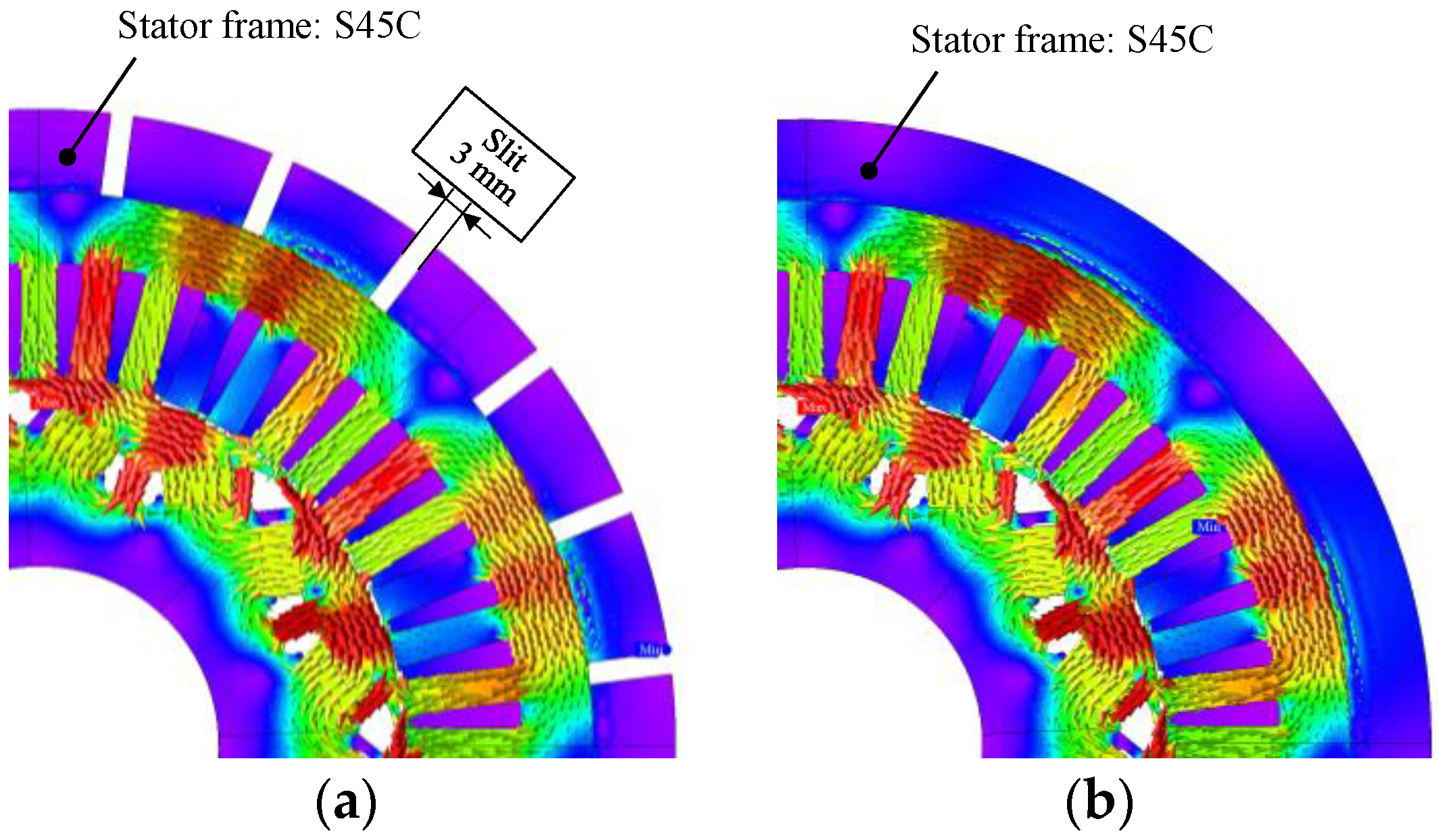
Figure 8 shows the rotor and the stator of the prototype motor. The rotor cores were skewed at an angle of 3.75 deg, taking advantage of the construction whereby the rotor is split into two parts. Thereby, 12th order space harmonics could be reduced because the angle between the teeth and the slots of the stator core was 3.75 deg. The gap between the stator core and the stator frame was minimized by inserting the stator core in the stator frame by shrink-fitting. Besides, slits were provided to the stator frame to suppress the iron loss. Figure 9 shows a magnetic flux density vector plot when a q-axis current of 80 A was supplied. However, the rotating speed was 1000 r/min. The model shown in Figure 9a had slits and the model shown in Figure 9b did not. As illustrated in Figure 9, by providing the slits, the armature flux passing in a circumferential direction could be reduced. Figure 10 shows an eddy current loss of the stator frames of the two models. The eddy current loss of the model with slits was 40.4% lower than that of the model without slits. It can be seen, from this result, that the slits were helpful in terms of iron loss.

3. Back E.m.f. Characteristic

3.1. Analysis of Back E.m.f.

Figure 11 shows the rotor geometry of the prototype motor model. It is crucial to design appropriately the saturation areas A and B shown in Figure 11 because the motor with the proposed adjustable field method achieves the magnetic field control by modulating the permeability of the magnetic leakage paths in the saturation areas. As shown in Figure 11, in the prototype motor, the width of the magnetic leakage paths in saturation area A was 3.2 mm and the widths of saturation area B were 1.5 mm and 0.5 mm. As shown in

Table 2. Width of magnetic leakage paths in saturation areas A and B.

Model	Saturation Area A	Saturation Area B
Model 1	2.1 mm	1.00 mm, 0.5 mm
Model 2	2.7 mm	1.25 mm, 0.5 mm
Model 3	3.7 mm	1.75 mm, 0.5 mm
Model 4	4.3 mm	2.00 mm, 0.5 mm

, the widths were parametrically changed to investigate the relationship between the width and the proposed motor performance.

Figure 12 shows the analysis results of the magnetic field Ψ_a. As shown in Figure 12, the minimum Ψ_a was determined with the width of the magnetic leakage paths. On the other hand, in all models, the gradient in the Ψ_a decreased when the Ψ_a was about 39.6 mWb. Therefore, the maximum Ψ_a was set at 39.6 mWb for all models to evaluate the performances with the same maximum fundamental component of the air gap flux.

Table 3. Magnetic field control performances of proposed motor models.

Parameter		Model 1	Model 2	Prototype Model	Model 3	Model 4
Max. Ψa	im (A)	8.1	8.9	10.0	10.5	11.7
	Ψa (mWb)	39.6	39.6	39.6	39.6	39.6
	Copper loss (W)	118	143	180	198	246
Min. Ψa	im (A)	0	0	0	0	0
	Ψa (mWb)	25.4	21.7	19.4	15.4	12.3
	Copper loss (W)	0	0	0	0	0
Controllable range of Ψa (mWb)		14.2	17.9	20.2	24.2	27.3

shows the copper losses and controllable ranges of the Ψ_a of each model. As shown in Table 3, the relationship between the controllable range of the Ψ_a and the copper loss for the magnetic field control was a trade-off. Therefore, when the proposed motor is designed to increase the controllable range, the motor efficiency deteriorates and the motor volume is enormous.

The ultimate design target of the proposed motor when the F_m is given is to output a large Ψ_a equivalent to when the saturation areas A and B shown in Figure 11 are replaced with air. In addition, the ideal design without the F_m is to leak a much larger PM flux on the rotor core, equivalent to when the saturation areas A and B are replaced with 35JNE230. Therefore, the prototype motor shown in Figure 11 was compared with these two ideal designs. Figure 12 shows the magnetic field amount of the motor with saturation areas replaced with air or 35JNE230. There was a difference in the magnetic field quantity and the magnetic field quantity of the prototype motor was inferior to that of the models simulating the ideal design. Regarding the rotor geometry of the prototype motor, only the widths of the magnetic leakage paths were parametrically adjusted to make the controllable range 50% of the maximum magnetic field amount while considering the mechanical strength. In other words, there is still room to consider other elements, such as PM shape, a flux barrier position, etc. Therefore, the optimized design of the IPMSM with the proposed adjustable field method will be investigated in future works.

3.2. Back E.m.f. Measurement Test

Figure 13 shows an experimental setup used in this paper. In the measurement test, the prototype motor was connected with a torque transducer TMNR-50NM, MinebeaMitsumi Inc. (Tokyo, Japan) and a load motor and the rotating speed of the prototype motor was controlled by the load motor. In this section, the back e.m.f. of the prototype motor was investigated by opening the terminal of the prototype motor and measuring the phase voltage. As mentioned above, the m.m.f. source F_m for magnetic field control was required in addition to the armature m.m.f. source. The F_m was supplied by the DC voltage supply.

Figure 14 shows waveforms and FFT results of the back e.m.f. when an F_m of 0 AT or 1200 AT was given to the modulation winding. However, the rotating speed was controlled at a constant speed of 1000 r/min by the load motor. It can be confirmed, from Figure 14, that the experimental value corresponded reasonably well with the analysis value and the fundamental component of the back e.m.f. increased by supplying the F_m. The fundamental components of experimental values without the F_m were approximately 3% smaller than that of the analysis value. This decrement of the e.m.f. was possibly caused by the manufacturing error of the width of the magnetic leakage paths and the air gap length. In addition, the mesh used in the FEM was also a factor that may have caused the error. On the other hand, the fundamental component of the back e.m.f. with the F_m of 1200 AT was 2.1 times larger than that without the F_m. Therefore, this result indicates that the prototype motor had a wide controllable range of the magnetic field.

Figure 15 illustrates the relationship between the magnetic field Ψ_a and the modulation current i_m of the prototype motor. As can be seen in the figure, the Ψ_a depends on the absolute value of i_m and can be approximated as

$${\Psi }_a\left(i_m\right)=-1.84\times {10}^{-3}{\left|i_m\right|}^4+0.39{\left|i_m\right|}^2+18.7 (\mathrm{mWb})$$

(1)

3.3. Magnetic Field Control Performance Comparison with Other Methods

In this section, based on the back e.m.f. measurement test results, the magnetic field control performance of the prototype motor was compared with that of the motor with other magnetic field control methods. The proposed motor was compared with three motors based on conventional techniques. The first benchmark was a conventional IPM motor. The magnetic field of the conventional IPM motor was weakened with a negative i_d. The second benchmark motor was a hybrid motor proposed in the reference [5,6]. The gap magnetic flux density of the hybrid motor was adjusted by the field current i_f. The third benchmark motor was a variable leakage flux motor introduced in the reference [7]. The magnetic leakage paths were provided in the rotor and the leakage PM flux could be adjusted by q-axis m.m.f. Therefore, the magnetic field of the variable leakage flux IPM motor was a function of the q-axis current i_q.

Figure 16, Figure 17 and Figure 18 show analysis models of the conventional IPM motor, the hybrid motor and the variable leakage flux motor, respectively. In addition,

Table 4. Specifications of compared motors.

Parameter		Prototype Motor	Conventional IPM Motor	Hybrid Motor	Variable Leakage Flux Motor
Manipulating variable for magnetic field control		Modulation current	d-axis current	Field current	q-axis current
		im	id	if	iq
Stator core diameter (mm)		ϕ148	←	←	←
Stack length (mm)		63	48	55.8	48
		(Core stack length: 48)		(Core stack length: 48)
Number of turns	Armature winding	6 turns/slot	←	←	←
	Additional winding	120 turns	-	120 turns	-
Core volume (mm3)		577,000	564,000	542,000	572,000
Copper volume (mm3)	Armature winding	337,000	307,000	323,000	307,000
	Additional winding	59,000	-	31,000	-
PM volume (mm3)		36,000	←	←	←
Magnetic circuit volume (mm3)		1,440,000	908,000	1,370,000	915,000
Max. current density (Arms/mm2)		20	←	←	←
Resistance	Armature winding	0.150	0.137	0.144	0.137
(Ω)	Additional winding	1.80	-	4.29	-
Max. torque (Nm)		12.2 (im = 10 A, iq = 80 A)	14.4 (iq = 80 A)	16.6 (if = 4.2 A, iq = 80 A)	13.9 (iq = 80 A)

shows the specifications of the compared motors. For a fair comparison, all motors had the same material, stator geometry, core stack length, number of winding turns, PM volume and maximum current density. The rotor bridge of the conventional IPM motor was set at 1.0 mm, considering mechanical strength. Because a 3D magnetic circuit and an additional winding were not needed, the stack length and the armature winding resistance of the conventional IPM motor and the variable leakage flux motor were lower than the proposed motor and the hybrid motor. When designing an SPM motor that rotates at higher than 10,000 r/min, it is common to use a protection tube for the rotor to prevent the PM from scattering. Therefore, the air gap length is usually designed longer than the IPM motor. In this paper, the air gap length of the prototype motor, the conventional IPM motor and the variable leakage flux motor was 0.7 mm and that of the hybrid motor was 1.0 mm. It can be seen, from Table 4, that the prototype motor was inferior in terms of torque density because the motor volume, including the 3D magnetic circuit, was the most enormous and output torque was the lowest among all analysis models. The deterioration of the output torque of the prototype motor was greatly affected by the magnetic saturation of the stator teeth due to the radial modulation flux.

Figure 19 shows the relationship between the Ψ_a and the manipulating variable of the Ψ_a of the compared motors. However, in the conventional IPM motor, the Ψ_a could not be directly controlled and the i_d was used to weaken the d-axis flux Ψ_d. As shown in Figure 15, a Ψ_a of 20.5 mWb could be adjusted in the prototype motor by supplying an i_m of 10 A. As shown in Figure 19a, in the conventional IPM motor, a Ψ_d of 20.5 mWb was weakened with an i_d of −63 A. In addition, from Figure 19b, in the hybrid motor, the maximum Ψ_a was 53.0 mWb when an i_f of 4.2 A was supplied and the minimum Ψ_a was 32.3 mWb when an i_f of −4.2 A was supplied. Thus, a Ψ_a of 20.7 mWb could be controlled by an i_f from −4.2 A to 4.2 A. On the other hand, as shown in Figure 19c, in the variable leakage flux motor, even if a maximum i_q of 80 A was supplied, it was not possible to control a Ψ_a of 20.5 mWb, which was roughly the same as the other motors. From this result, the variable leakage flux motor had a drawback in terms of the controllable range of the magnetic field.

Table 5. Comparison results of magnetic field control performance.

Parameter		Prototype Motor	Conventional IPM Motor	Hybrid Motor	Variable Leakage Flux Motor
Max. Ψa or Max. Ψd	Variable value (A)	im = 10	id = 0	if = 4.2	iq = 80
	Ψa or Ψd (mWb)	Ψa = 39.6	Ψd = 41.7	Ψa =53.0	Ψa = 43.5
	Copper loss (W)	180	0	75.7	877
Min. Ψa or Min. Ψd	Variable value (A)	im = 0	id = −63	if = −4.2	iq = 0
	Ψa or Ψd (mWb)	Ψa = 19.1	Ψd = 21.2	Ψa =32.3	Ψa = 33.3
	Copper loss (W)	0	544	75.7	0
Controllable range of Ψa or Ψd (mWb)		20.5	20.5	20.7	10.1

shows the comparison result of the magnetic field control performance when a Ψ_a of around 20.5 mWb was adjusted. However, as described above, the limit value of the magnetic field control range was 10.1 mWb in the variable leakage flux motor. It can be seen, from Table 5, that the copper loss when the Ψ_a was around 20.5 mWb was 180 W for the proposed motor and 151 W for the hybrid motor, while it was 544 W for the conventional IPM motor. In other words, the proposed motor and the hybrid motor had higher magnetic field control performance.

Figure 20 shows a vector plot of magnetic flux density when the rotor shafts of the prototype motor and the hybrid motor were most strongly magnetized. Although the rotor shaft diameter of the hybrid motor was larger than that of the prototype motor, the magnetic flux density of the hybrid motor rotor shaft was much higher than the prototype motor. Only the modulation flux passed through the rotor shaft in the prototype motor. On the other hand, in addition to the field flux, the PM flux penetrated to the rotor shaft of the hybrid motor. Therefore, the flux passing through the rotor shaft of the hybrid motor was higher than that of the prototype motor, resulting in a large diameter design for the rotor shaft. Figure 21 shows the B–H curve of the N39UH used for the PM and the operating points of the PM when magnetic field control was carried out in each compared model. The PM of the hybrid motor was easily demagnetized due to a low permeance coefficient caused by a wide air gap. On the other hand, it can be seen that the PM in the prototype motor was hardly demagnetized even if the same amount of the Ψ_a was weakened by applying the conventional field weakening control to the IPM motor.

4. Drive System of Prototype Motor

From Equation (1), it can be seen that the magnetic field of the proposed motor depends on the absolute value of the i_m. Therefore, this paper examines magnetic field control methods by supplying the DC i_m.

The DC i_m was controlled with the DC power supply ZX-800L, Takasago Ltd. and the armature currents were supplied by the three-phase inverter MWINV-5R022, Myway Plus Corporation. The electrical conditions and the control block diagram are shown in

Table 6. Experimental conditions of current control of prototype motor.

Parameter	Symbol	Value
DC-bus voltage	Vdc	270 V
Dead time	td	4 μs
Switching frequency	fsw	10 kHz
Crossover frequency of current control	ωc	4000 rad/s

and Figure 22, respectively. As shown in Table 6, the dead time was 4 μs and the error voltage of the dead time was compensated based on the reference [18,19]. In addition, as shown in Figure 22, the relationship between the Ψ_a and i_m expressed in Equation (1) was used for the decoupling item.

Figure 23 shows the experimental results at the rotating speed of 1000 r/min when an i_m of 0 A or 6 A, an i_d of 0 A and an i_q of 20 A were given to the prototype motor. It can be confirmed from the waveforms of the three-phase line currents and i_m that the line currents could be controlled regardless of the i_m.

Table 7. Comparison of output torque.

Modulation Current	q-Axis Current	Output Torque
DC 0 Adc	20 A	1.49 Nm
DC 6 Adc	20 A	2.40 Nm

shows the output torque T_ave when a DC i_m of 0 A_dc or 6 A_dc was given to the modulation winding. As shown in Table 7, the output torque increased from 1.49 Nm to 2.40 Nm by supplying a DC i_m of 0 A_dc or 6 A_dc. This result reveals that the prototype motor could control the Ψ_a by the DC i_m because the T_ave increased with the DC i_m under the same armature current condition.

In this section, based on the relationship between the Ψ_a and the i_m, the drive system for the prototype motor is examined. The above results show that the drive system shown in Figure 22 could control the line currents independently of the DC i_m.

Moreover, Equation (1) means that the square wave i_m can be used to output the constant Ψ_a because the absolute value of the square wave is constant. The ability to control the Ψ_a with the square wave i_m is one of the unique points of the proposed adjustable field method. In other words, the power electronics for the proposed motor have a lot of flexibility. The proposed motor can be driven by different power electronics, optimized for magnetic field adjustment by taking advantage of the flexibility. Therefore, we will study the suitable drive system for the proposed motor in the near future. When the power electronics circuit is optimally designed for the field adjustment, the number of switching devices and the complexity of the circuit must be deeply considered because they easily deteriorate the total efficiency [20].

5. Load Characteristics

5.1. Load Analysis

Figure 24 shows the relationships between i_q and torque T characteristic (I–T characteristic) of the proposed motor models with different magnetic leakage path widths shown in Figure 11 and Table 2. Figure 24a shows the I–T characteristics when the F_m was not supplied. From this Figure, it can be seen that the torque constant, which is defined as the gradient of the I–T characteristic, depended on the minimum Ψ_a shown in Table 3. Figure 23b shows the I–T characteristics with F_m. The torque constant was the same among all models because the maximum Ψ_a was unified to 39.6 mWb for all models. However, the required F_m was more significant for smaller minimum Ψ_a.

Figure 25 shows the relationships between rotating speed N and T characteristic (N–T characteristic) of the proposed motor models when the maximum i_q of 80 A was applied. Figure 25a shows the N–T characteristics without the F_m. As shown in the Figure, the model with the smaller minimum Ψ_a had a wider high-speed operating range. On the other hand, as can be seen in Figure 25b, for the same reason valid for the I–T characteristic, the N–T characteristics with the F_m were the same for all models.

It is confirmed, from this result, that the prototype motor model could achieve the low-speed high-torque operation when the F_m was given and the high-speed low-torque operation when the F_m was not given. In addition, in comparing the models with the same maximum Ψ_a and the different controllable range of the Ψ_a, it could be revealed that the copper volume and the copper loss for the magnetic field control were in a trade-off relationship with the motor operating range.

The losses at the low-speed high-torque operating point X and the high-speed low-torque operating point Y shown in Figure 25 were evaluated in comparison with the losses of other compared models shown in Figure 16, Figure 17 and Figure 18.

Table 8. Current condition in load analysis.

Operating Point	Prototype Motor	Conventional IPM Motor	Hybrid Motor	Variable Leakage Flux Motor
X	im = 10 A, iq = 63 A	id = 0.0 A, iq = 58 A	if = 4.2 A, iq = 47 A	iq = 62 A
Y	im = 0.0 A, iq = 13 A	id = −63 A, iq = 10 A	if = −4.2 A, iq = 7.7 A	iq = 7.5 A

shows the current conditions at each operating point. At the operating point X, the current that maximized the Ψ_a of each motor was supplied and, at the operating point Y, the current that minimized the Ψ_a was supplied. Figure 26 shows the loss analysis results. In this paper, the analysis method of iron loss was common to all motors. The hysteresis loss of the electromagnetic steel sheet 35JNE230 was calculated by considering its hysteresis loop. On the other hand, there are no data about the hysteresis loops of the carbon steel S45C and the PM N39UH in JMAG-Designer. Therefore, the iron loss of these parts included only the eddy current loss. Figure 26a shows the loss analysis results at the operating point X. The copper loss of the prototype motor was significant at the operating point X because the F_m was necessary to cause the magnetic saturation and increase the Ψ_a. In addition, the copper loss of the armature winding was also the largest because the maximum Ψ_a of the prototype motor was the smallest among the compared motors, as can be seen in Table 5. The modulation flux penetrated to the PM when the F_m was given. However, there was almost no increase in PM eddy current loss due to the modulation flux because the modulation flux was a DC. For the same reason, additional losses of the stator frame and rotor shaft due to the modulation flux were also small. Figure 26b shows the loss analysis results at the operating point Y. Because the negative i_d was supplied to the conventional motor at the operating point Y, the conventional IPM motor delivered the reluctance torque in addition to the PM torque. Therefore, the conventional IPM motor was advantageous over the other motors at the operating point Y. However, in the high-speed range, the loss of the prototype motor was the smallest among the compared motors because the additional m.m.f. was not necessary to decrease the Ψ_a. The PM eddy current loss of the hybrid motor was higher than the other benchmark IPM motors because of the SPM structure. Therefore, the PMs of the hybrid motor were prone to de-magnetization due to heat in addition to the temperature rise of the PMs as well as the counter magnetic field to the PMs.

The above results show that the proposed motor could be driven at a high-speed range with less copper loss and iron loss than the field weakening control and the other adjustable field methods. However, in the analysis using FEM, there was often a difference in iron loss between the experimental and the analysis. Therefore, as a future task, it is necessary to accurately measure the drive system’s efficiency and evaluate the prototype motor’s performance in more detail [21].

5.2. Load Test

Figure 27 shows the experimental result of the I–T characteristic. In the actual load test, to evaluate the performance of the prototype motor as an adjustable field IPMSM, the i_d was not included in the armature current. Besides, the maximum i_q was 24 A due to the current limitation of the three-phase inverter MWINV-5R022. The prototype motor was controlled at 1000 r/min by the load motor. The F_m was supplied by the DC power supply, similar to the measurement test of the back e.m.f. As shown in Figure 25, the experimental value was in good agreement with the analysis value except in the low F_m condition. The torque constant could be changed according to the F_m. There was a difference between the experimental and analysis values when the F_m was 0 AT or 360 AT. The leading cause of the difference is the decrement of Ψ_a due to the production and mesh error found in the measurement test of the back e.m.f. From the above results, it is confirmed that the prototype motor could control the torque constant freely according to the F_m.

Figure 28 shows the experimental result of the N–T characteristic. The phase voltage at most 30 V was supplied to the prototype motor assuming an input DC bus voltage of 60 V, because the maximum rotating speed was as low as 3000 r/min due to the speed limitation of the load system. In addition, the maximum torque was 3.7 Nm because the maximum i_q was 24 A due to the current limitation of the inverter. Since the analysis did not consider iron loss and mechanical loss, the torque of the analysis result was slightly larger than that of the experimental result over the entire N–T characteristic. Especially with a large F_m, the harmonics were also high. Therefore, the difference between the observed and analysis values became large. In addition, when the F_m was low, the measured magnet torque was slightly lower than the analyzed value because the Ψ_a was smaller than expected due to the production error, similar to the I–T characteristic measurement test. However, the tendency of the N–T characteristic was in good agreement.

Based on the above results, it can be seen that the proposed motor could achieve both the low-speed high-torque and the high-speed low-torque operation according to the F_m.

6. Conclusions

In this paper, the essential operating characteristics of the IPMSM with the proposed adjustable field method utilizing magnetic saturation were examined by conducting the measurement test of the back e.m.f. and the actual load tests.

As a result of the back e.m.f. measurement test, it was confirmed that 51.7% of the Ψ_a of the prototype motor was controllable. Based on the test results, the magnetic field control performance was compared with the field weakening control and other adjustable field methods under the same amount of the magnetic field control. The proposed method has some advantages, such as a broader controllable range of magnetic field, less copper loss and anti-demagnetization capability. Detailed contributions of the proposed motor are as follows:

• Controllable range of the proposed motor magnetic field was 103% larger than that of the variable leakage flux motor, as shown in Table 5;
• Copper loss enhancement of the proposed method was up to 66.9% compared to the conventional field weakening control, as shown in Table 5;
• The proposed motor had a higher anti-demagnetization capability than the hybrid motor by 6.5%, as shown in Figure 20 and Figure 21.

In addition, the losses of the proposed motor at two operating points, which are the low-speed high-torque point and the high-speed low-torque point, were compared with that of the benchmarks. As a result, it was seen that the copper loss of the proposed motor was the largest among the compared motors at the low-speed high-torque operating point. On the other hand, the efficiency considering the copper loss and the iron loss of the proposed motor was the highest at the high-speed low-torque operating point.

In the actual load test, the I–T characteristic and the N–T characteristic were measured. It was confirmed through the I–T characteristic measurement test that the torque constant of the prototype motor could be varied continuously according to the F_m. Besides, from the measurement test of the N–T characteristic, it can be seen that the prototype motor could change the operating characteristics, which are the low-speed high-torque and the high-speed low-torque, depending on the F_m. However, the actual load test considering the reluctance torque was not conducted. In the adjustable field PMSM, the conventional vector controls, such as maximum torque per ampere (MTPA) control, maximum torque per voltage (MTPV) control and field weakening control, considered under the constant Ψ_a condition, had to be extended because the Ψ_a was adjustable. Therefore, the derivation of the extended vector control algorithm for the adjustable field PMSM is an essential topic for future work.

References

1. Pellegrino, G.; Vagati, A.; Guglielmi, P.; Boazzo, B. Performance Comparison between Surface-Mounted and Interior PM Motor Drives for Electric Vehicle Application. IEEE Trans. Ind. Appl. 2012, 59, 803–811. [Google Scholar] [CrossRef] [Green Version]
2. Fatemi, A.; Ionel, D.M.; Popescu, M.; Chong, Y.C.; Demerdash, N.A.O. Design Optimization of a High Torque Density Spoke-Type PM Motor for a Fomula E Race Drive Cycle. IEEE Trans. Ind. Appl. 2018, 54, 4343–4354. [Google Scholar] [CrossRef]
3. Jo, C.; Seol, J.Y.; Ha, I.J. Flux-Weakening Control of IPM Motors with Significant Effect of Magnetic Saturation and Stator Resistance. IEEE Trans. Ind. Electron. 2008, 55, 1330–1340. [Google Scholar]
4. Sue, S.M.; Pan, C.T. Voltage-Constraint-Tracking-Based Field-Weakening Control of IPM Synchronous Motor Drives. IEEE Trans. Ind. Electron. 2008, 55, 340–347. [Google Scholar] [CrossRef]
5. Mizuno, T.; Nagayama, K.; Ashikaga, T.; Kobayashi, T. Basic Principles and Characteristics of Hybrid Excitation Type Synchronous Machine. IEEJ Trans. Ind. Appl. 1995, 115, 1402–1411. [Google Scholar] [CrossRef] [Green Version]
6. Tapia, J.A.; Leonardi, F.; Lipo, T.A. Consequent-Pole Permanent-Magnet Machine with Extended Field-Weakening Capability. IEEE Trans. Ind. Appl. 2003, 39, 1704–1709. [Google Scholar] [CrossRef] [Green Version]
7. Kato, T.; Hijikata, H.; Minowa, M.; Akatsu, K.; Lorenz, R.D. Design Methodology for Variable Leakage Flux IPM for Automobile Traction Drives. In Proceedings of the 2014 Energy Conversion Congress and Exposition–ECCE, Pittsburgh, PA, USA, 14–18 September 2014; pp. 3548–3555. [Google Scholar]
8. Aoyama, M.; Noguchi, T. Automatic Variable Magnetic Flux Technique in Consequent Pole Type PM-Motor Utilizing Space Harmonic. In Proceedings of the 2018 International Symposium on Power Electronics, Electrical Drives, Automation, and Motion–SPEEDAM, Amalfi, Italy, 20–22 June 2018; pp. 1315–1320. [Google Scholar]
9. Hijikata, H.; Saka, Y.; Akatsu, K.; Miyama, Y.; Arita, H.; Daikoku, A. Multi-Phase Inverter-Fed MATRIX Motor for High Efficiency Driving. IEEJ Trans. Ind. Appl. 2018, 138, 257–264. [Google Scholar] [CrossRef]
10. Sakai, K.; Hashimoto, H.; Kuramochi, S. Principle and Basic Characteristics of Variable-Magnetic-Force Memory Motors. IEEJ Trans. Ind. Appl. 2011, 131, 53–60. [Google Scholar] [CrossRef]
11. Zhu, X.; Xiang, Z.; Quan, L.; Wu, W.; Du, Y. Multimode Optimization Design Methodology for a Flux-Controllable Stator Permanent Magnet Memory Motor Considering Driving Cycles. IEEE Trans. Ind. Electron. 2018, 65, 5353–5366. [Google Scholar] [CrossRef]
12. Iwama, K.; Noguchi, T. Performance Comparison between Adjustable Field IPM Motor Based on Permeability Modulation Technique and Conventional IPM Motor. In Proceedings of the 23rd International Conference on Electrical Machines and Systems–ICEMS, Hamamatsu, Japan, 24–27 November 2020; pp. 1418–1423. [Google Scholar]
13. Chen, X.; Wang, J.; Sen, B.; Lazari, P.; Sun, T. A High-Fidelity and Computationally Efficient Model for Interior Permanent-Magnet Machines Considering the Magnetic Saturation, Spatial Harmonics, and Iron Loss Effect. IEEE Trans. Ind. Electron. 2015, 62, 4044–4055. [Google Scholar] [CrossRef]
14. Liang, P.; Chai, F.; Li, Y.; Pei, Y. Analytical prediction of magnetic field distribution in spoke-type permanent-magnet synchronous machines accounting for bridge saturation and magnet shape. IEEE Trans. Ind. Electron. 2017, 64, 3479–3488. [Google Scholar] [CrossRef]
15. Hemeida, A.; Lehikoinen, A.; Rasilo, P.; Vansompel, H.; Belahcen, A.; Arkkio, A.; Sergeant, P. A Simple and Efficient Quasi-3-D Magnetic Equivalent Circuit for Surface Axial Flux Permanent Magnet Synchronous Machines. IEEE Trans. Ind. Electron. 2019, 66, 8318–8333. [Google Scholar] [CrossRef]
16. Alipour-Sarabi, R.; Nasiri-Gheidari, Z.; Oraee, H. Development of a three-dimensional magnetic equivalent circuit model for axial flux machines. IEEE Trans. Ind. Electron. 2020, 67, 5758–5767. [Google Scholar] [CrossRef]
17. Shokrollahi, H.; Janghorban, K. Soft magnetic composite materials (SMCs). J. Mater. Process. Technol. 2007, 189, 1–12. [Google Scholar] [CrossRef]
18. Diao, N.; Sun, X.; Song, C.; Zhang, Q.; Zhang, Z. A Multi-modulation Times SVPWM for Dead Time Effect Elimination in Three-level Neutral Point Clamped Converters. IEEE Trans. Ind. Electron. 2021, 68, 5476–5485. [Google Scholar] [CrossRef]
19. Oto, Y.; Noguchi, T.; Sasaya, T.; Yamada, T.; Kazaoka, R. Space Vector Modulation of Dual-Inverter System Focusing on Improvement of Multilevel Voltage Waveforms. IEEE Trans. Ind. Electron. 2019, 66, 9139–9148. [Google Scholar] [CrossRef]
20. Mapelli, F.L.; Tarsitano, D.; Mauri, M. Plug-In Hybrid Electric Vehicle: Modeling, Prototype Realization, and Inverter Losses Reduction Analysis. IEEE Trans. Ind. Electron. 2009, 57, 598–607. [Google Scholar] [CrossRef]
21. Caruso, M.; Tommaso, A.O.D.; Lisciandrello, G.; Mastromauro, R.A.; Miceli, R.; Nevoloso, C.; Spataro, C.; Trapanese, M. A General and Accurate Measurement Procedure for the Detection of Power Losses Variations in Permanent Magnet Synchronous Motor Drives. Energies 2020, 13, 5770. [Google Scholar] [CrossRef]
Figure 1. B–H curve of 35JNE230.
Energies 15 00052 g001
Figure 2. Magnetic circuit of prototype motor.
Energies 15 00052 g002
Figure 3. Vector plot of modulation flux with Fm of 1200 AT: (a) modulation flux; (b) leakage modulation flux passing through air.
Energies 15 00052 g003
Figure 4. DC flux in rotor: (a) usual DC flux; (b) radial DC flux.
Energies 15 00052 g004
Figure 5. Variation in magnetic flux: (a) usual DC flux; (b) radial DC flux.
Energies 15 00052 g005
Figure 6. Vector plot of magnetic flux density: (a) PM flux without Fm; (b) PM and modulation flux with Fm of 720 AT; (c) PM and modulation flux with Fm of 1200 AT.
Energies 15 00052 g006
Figure 7. Gap magnetic flux density: (a) waveforms; (b) FFT results.
Energies 15 00052 g007
Figure 8. Configuration of prototype motor: (a) photograph of rotor; (b) photograph of stator.
Energies 15 00052 g008
Figure 9. Magnetic flux density vector on x–y cross-section with q-axis current of 80 A: (a) with slit; (b) without slit.
Energies 15 00052 g009
Figure 10. Eddy current loss of stator frame with q-axis current of 80 A.
Energies 15 00052 g010
Figure 11. Magnetic saturation areas of prototype motor.
Energies 15 00052 g011
Figure 12. Magnetic fields of proposed motor models with different magnetic leakage path widths.
Energies 15 00052 g012
Figure 13. Experimental setup.
Energies 15 00052 g013
Figure 14. U-phase back e.m.f. at rotating speed of 1000 r/min: (a) waveforms; (b) FFT results.
Energies 15 00052 g014
Figure 15. Experimental result of Ψa and its approximate line.
Energies 15 00052 g015
Figure 16. Analysis model of conventional IPM motor.
Energies 15 00052 g016
Figure 17. Analysis model of hybrid motor.
Energies 15 00052 g017
Figure 18. Analysis model of variable leakage flux motor.
Energies 15 00052 g018
Figure 19. Relationship between magnetic field and variable for magnetic field control: (a) conventional IPM motor with field weakening control; (b) hybrid motor; (c) variable leakage flux motor.
Energies 15 00052 g019
Figure 20. Analysis results of magnetic flux density: (a) prototype motor rotor shaft with im of 10 A; (b) hybrid motor rotor shaft with if of −4.2 A.
Energies 15 00052 g020
Figure 21. B–H characteristic of N39UH and PM operating points of each compared motor.
Energies 15 00052 g021
Figure 22. Control block diagram of current control of prototype motor when using DC im.
Energies 15 00052 g022
Figure 23. Experimental results of current control: (a) with iq of 20 A and im of 0 A; (b) with iq of 20 A and im of 6 A.
Energies 15 00052 g023
Figure 24. I–T characteristics of proposed motor models with different magnetic leakage path widths: (a) without Fm; (b) with Fm.
Energies 15 00052 g024
Figure 25. N–T characteristics of proposed motor models: (a) without Fm; (b) with Fm.
Energies 15 00052 g025
Figure 26. Loss analysis results: (a) loss at operating point X; (b) loss at operating point Y.
Energies 15 00052 g026
Figure 27. Experimental results of I–T characteristic.
Energies 15 00052 g027
Figure 28. Experimental results of N–T characteristic.
Energies 15 00052 g028