Abstract
The main goal of this research was to propose a new method of polarimetric SAR data decomposition that will extract additional polarimetric information from the Synthetic Aperture Radar (SAR) images compared to other existing decomposition methods. Most of the current decomposition methods are based on scattering, covariance or coherence matrices describing the radar wave-scattering phenomenon represented in a single pixel of an SAR image. A lot of different decomposition methods have been proposed up to now, but the problem is still open since it has no unique solution. In this research, a new polarimetric decomposition method is proposed that is based on polarimetric signature matrices. Such matrices may be used to reveal hidden information about the image target. Since polarimetric signatures (size 18 × 9) are much larger than scattering (size 2 × 2), covariance (size 3 × 3 or 4 × 4) or coherence (size 3 × 3 or 4 × 4) matrices, it was essential to use appropriate computational tools to calculate the results of the proposed decomposition method within an acceptable time frame. In order to estimate the effectiveness of the presented method, the obtained results were compared with the outcomes of another method of decomposition (Arii decomposition). The conducted research showed that the proposed solution, compared with Arii decomposition, does not overestimate the volume-scattering component in built-up areas and clearly separates objects within the mixed-up areas, where both building, vegetation and surfaces occur.
1. Introduction
Nowadays, satellite data are one of the main sources of information about Earth’s surface and processes that occur in the environment. A multitude of environmental phenomena that can be studied from above is ensured thanks to a broad spectrum of different kinds of devices and systems that are placed on satellites. One of those systems is synthetic aperture radar (SAR) [1]. SAR emits its own electromagnetic radiation toward Earth’s surface and records the signal that is backscattered by objects located on the ground. SAR saves information about the amplitude (Am) and the phase (ϕ) of the returning signal for each pixel of generated radar image. Those parameters are used in the most widely known methods of SAR data processing: InSAR (interferometry SAR) [2], DInSAR (differential interferometry SAR) [2] and PSI (permanent/persistent scatterers interferometry) [3]. The first mentioned method, InSAR, is used to generate digital elevation models (DEMs), and the second and third allow for determination of the values of vertical ground deformations with millimetre accuracy. Since 1979, when the Seasat satellite equipped with the first SAR system was launched, enormous progress has been made associated with satellite radar imaging. During these almost 40 years, many new SAR systems have been constructed and exploited, among them, those placed on ERS-1, ERS-2, ENVISAT and Sentinel-1 satellites belonging to the European Space Agency (ESA), TerraSAR-X and TanDEM-X (German Space Agency-DLR), Radarsat-1 and Radarsat-2 (Canadian Space Agency - CSA), ALOS-1 and ALOS-2 (Japanese Space Agency - JAXA) or in the constellation of COSMO-SkyMed satellites that belong to the Italian Space Agency (ASI). Some of those systems have already completed their missions (ERS-1, ERS-2, ENVISAT, ALOS-1, Radarsat-1), and some of them (e.g., ALOS-2, Sentinel-1) are at the beginning of their missions. The images gathered by the currently operating SAR systems are characterized by impressive spatial resolution (even less than 1 m) and much shorter revisit time (i.e., better temporal resolution). Additionally, extra information about polarization of transmitted and received waves is gathered, which constitutes the science of SAR polarimetry (PolSAR) [4]. All these improvements make current SAR systems a source of more complete and accurate information about imaged targets or phenomena on the Earth’s surface, which make it very important in geosciences. However, the amount and the high quality of provided data pose a challenge in terms of optimal processing. In this context, optimal processing needs to be understood as an extraction of as much information as possible about the Earth’s surface from satellite data in reasonable time. This means that new, more advanced processing algorithms need to be developed, and the most recent achievements in computer science should be exploited. This mentioned challenge constitutes the incentive to undertake the research described in this paper.
The analysis presented in this work focuses on the problem of polarimetric SAR data decomposition procedures [4]. Decomposition is one of the most important steps of polarimetric SAR radar data processing because it directly determines the amount of information that can be extracted from the data. Its goal is to assess the amounts of each so-called canonical scattering mechanism in the received radar response corresponding to a single pixel of a SAR image. There has been a number of different polarimetric-decomposition methods already proposed in the literature. The most commonly used are Pauli [5], Freeman and Duren [6], Yamaguchi [7], Touzi [8], H/A/alpha [5] and Arii [9] decompositions. All of them are based on the scattering matrix or coherence/covariance matrix representing the received radar signal in each pixel of a SAR image. The scattering matrix has a size of 2 × 2, while coherence and covariance matrices have a size of 3 × 3 or 4 × 4. All of them are complex matrices. Despite the presence of many different decomposition methods, the problem of polarimetric data decomposition remains open since no unique solution for this issue exists. Different decomposition methods realize different approaches and are based on different assumptions, resulting in diverse outcomes. Usually, the results can be compared and assessed only in a relative manner.
In this work, a new method of polarimetric decomposition is proposed. It is not directly based on the analysis of scattering, coherence or covariance matrices but on polarimetric signatures. A polarimetric signature is a matrix 180 × 90 in size characterizing the radar wave-scattering process. It is computed based on the scattering matrix. Polarimetric signatures do not contain additional information comparing to scattering matrix, but they allow one to distinguish the subtle changes in scattering characteristics [10]. Analysis of polarimetric signatures may help to reveal some hidden information that can be used for a more unique description of the target [11]. In order to apply polarimetric signatures to decomposition, a specific method of solving the decomposition’s equations set also needs to be proposed. In this work, iterative methods were chosen due to the possibility of implementing complex constraints on the solution. Those assumptions led the authors to the following scientific question: does the application of polarimetric signatures in decomposition procedures, together with the proposed iterative methods for solving the decomposition equation set, provide additional information in the decomposition results in comparison to the methods based on scattering, coherence or covariance matrices? The search for the answer to this question was the main goal of the reported work.
In this work, two different iterative are proposed and tested to solve the decomposition problem using polarimetric signatures: simultaneous iterative reconstruction (SIRT) and simulated annealing (SA). Both methods start from a random, initial solution, but SIRT calculates corrections in each iteration in a deterministic way. For the SA algorithm, a correction vector is generated randomly and can be projected in a probabilistic way. The latter approach is more time-consuming but can be helpful for avoiding local minima of evaluation functions.
In order to speed up SIRT and SA calculations, the proposed approach makes use of the graphical processing unit (GPU) [12]. GPU is a specialized electronic circuit designed to rapidly manipulate and alter memory to accelerate the creation of images in a frame buffer intended for output to a display. GPUs are very often used for accelerating computations in specific applications.
The proposed approach to polarimetric decomposition has an innovative character due to the fact that it is based on polarimetric signatures (not scattering, covariance or coherence matrices), it makes use of mathematical methods—simulated annealing and SIRT—that have not yet been used in the polarimetric decomposition procedure, and finally, it utilizes a GPU card to accelerate the computations. The basic advantage of our approach is the decrease in volume overestimation in urban areas, together with a significant decrease in computational time.
The remainder of this paper is organized as follows. Section 2 contains the introduction to satellite radar polarimetry, polarimetric decomposition and the concept of polarimetric signatures. In Section 3, the new method of quad-polarimetric SAR data decomposition using simulated annealing and SIRT methods is proposed. The validation of developed decomposition using the synthetic and selected real input data, as well as analysis of obtained results, are presented and described in Section 4. Next, in Section 5, use of GPU to support decomposition optimization analysis is described. Section 6 describes the results of the tests for a real SAR scene. Finally, Section 7 summarizes and concludes this paper.
2. Polarimetric SAR
Radar polarimetry (PolSAR) is a relatively recent development in the field of active remote sensing systems [4]. Its aim is to gather information about physical properties of imaged surfaces based on analysis of polarization information of transmitted and backscattered waves. Such analysis allows for attainment of knowledge about the geometrical structure, orientation and physical properties of the scatterers. SAR systems can work in single-polarization (single-pol), dual-polarization (dual-pol) or quad-polarization (quad-pol) mode. In the first case, the transmitted radar wave is polarized in one way (vertically or horizontally), and the same polarization component of the returning wave is received by the system. Analogously, in dual-pol mode, one polarization is transmitted, and two orthogonal polarizations are received. The full polarimetric information about scatterers is gathered in the case of quad-pol SAR systems; when two orthogonal polarizations are transmitted, the same two are received. Since the presented work is related to the quad-pol mode, further descriptions are focused on this case.
For each pixel of radar image, the polarimetric information gathered by quad-polarimetric SAR systems is saved in the form of a 2 × 2 scattering matrix (S) with STrR elements (Equation (1)).
where Tr denotes transmitted polarization and R denotes received polarization. In the most popular linear basis, the vertically (v) and horizontally (h) polarized waves are used. Following this, for example, the Shh element of the scattering matrix represents backscatter response of the target for the case when the transmitted wave is horizontally polarized, and the horizontal component of the returning wave is recorded. The scattering matrix is a starting point for all further polarimetric analysis. In the case of pure or isolated scatterers, the polarimetric information can be directly extracted from the scattering matrix. However, in the case of distributed targets, the second-order statistics of the scattering matrix, i.e., covariance (Cov) (Equation (2)) or coherence matrix (Coh) (Equation (3)), need to be used. In Equations (2) and (3), * is used to denote conjugation, and ⟨ ⟩ means averaging in spatial window (e.g., 7 × 7 pixels).
Radar backscattering can also be described by Kennaugh (K) or Mueller (M) matrices. Similarly to the scattering matrix, they also represent the relation between the transmitted and scattered radar wave. The Kennaugh matrix is given by Equation (4), while the Mueller matrix is given by Equation (5).
where , , , , , , and .
Polarimetric SAR data have found numerous applications in geoscience. Data can be used to study, among other things, surface roughness [13], soil moisture [14] and land-cover classes [11]. In oceanography, polarimetric SAR images are used to analyse surface currents and wind field [15]. On the other hand, in forestry, they are used to estimate tree height [16]. Radar polarimetry also plays a crucial role in disaster monitoring, e.g., for oil spills [17] or fire detection [18].
2.1. Polarimetric Decomposition
In most cases, the single pixel of a SAR image represents the response from many individual scatterers that are located within a single corresponding resolution cell. Therefore, the measured scattering matrix and the derived covariance and coherence matrices are actually sums of corresponding matrices representing individual scatterers located within this resolution cell. In order to retrieve the information about those individual scatterers from the measured scattering/covariance/coherence matrix, the decomposition procedure is exploited. Polarimetric decomposition is one of the key steps of polarimetric SAR data processing since it directly affects the amount of information that can be extracted. The polarimetric decomposition procedure can generally be described as a representation of the measured scattering matrix or coherence/covariance matrix as a linear combination of simple components [4]. These components represent the scattering types: single-bounce (or even-bounce), double-bounce (or odd-bounce), helix scattering and volume scattering (Figure 1). The single-bounce scattering mechanism is characteristic for different kinds of surfaces, e.g., surfaces of lakes, roads, rivers, flat roofs or bare soils. The double-bounce scattering mechanism is, in turn, typical for vertical objects, e.g., building walls, lanterns, poles and other upright elements of engineering objects. The helix scattering mechanism occurs in the case of complex shapes of man-made objects, and finally, volume scattering can be used to identify different kinds of vegetation.
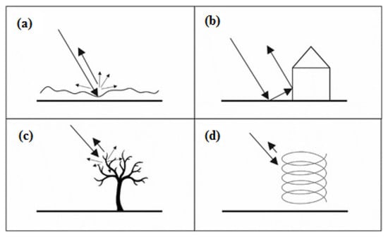
Figure 1.
Basic scattering types (a)—single-bounce, (b)—double-bounce, (c)—volume scattering, (d)—helix scattering).
A number of different decomposition methods have been proposed in the literature. They are divided into coherent and incoherent decompositions. Coherent decompositions are based on the scattering matrix, while incoherent decompositions use second-order statistics, coherence or covariance matrices. The most widely used decompositions are freeman and Durden’s decomposition [6], Yamaguchi’s decomposition [7], H/A/alpha decomposition [5], Touzi’s decomposition [8] or Arii decomposition [9]. All of them have their pros and cons, making their usefulness dependent mainly upon the types of targets being imaged [5]. Coherent decomposition presents good-quality single-bounce and double-bounce scattering identification [19]. Recognition of volume-scattering components by coherent decomposition is most inaccurate and sometimes overestimated in urban areas [20]. Incoherent decompositions, as with Freeman or Yamaguchi, are usually characterized by more accurate assessment of each scattering mechanism in the analyzed pixels. However, the problem of volume scattering overestimation in rotated built-up areas is present [21]. The same problems occur in the case of H/A/alpha decomposition [22]. In turn, H/A/alpha decomposition has the possibility of recognizing areas with mixed scattering mechanism by means of an HA image (product of entropy (H) and anisotropy (A)) [4]. Arii developed an adaptive-model-based decomposition method that could estimate both the mean orientation angle and a degree of randomness for the canopy scattering for each pixel in an SAR image. However, the problem of volume-scattering overestimation seems to still be present in the results, which are proved in Section 6. Since Arii’s decomposition is one of the most recent methods, built on top of the previous ones, it was chosen in this work to be compared with the proposed method based on polarimetric signatures.
The mentioned weaknesses of existing decomposition methods were the motivation to develop a new method that overcomes or at least decreases the following limitations: overestimation of volume scattering in built-up areas and problems with recognition of mixed areas.
2.2. Polarimetric Signatures
The concept of a polarimetric signature was introduced in 1978 by van Zyl et al. [10] as a tool for graphical representation of polarimetric information of the scatterer. The signature allows for full description of the polarimetric properties of imaged objects based on the measured scattering matrix by presenting the backscatter response at all possible combinations of transmitted and received polarizations. In order to facilitate the interpretation of this comprehensive information, the polarimetric signature is usually represented in two channels: co-polarized and cross-polarized. In the former case, the transmitted and received waves have the same polarization, and in the latter case, the polarizations are orthogonal.
In the polarimetric signature, which can be visualised as a 3D surface or saved in the form of a two dimensional matrix, the wave intensities are computed for all possible polarization states and parameterized by the polarization ellipse orientation angle (χ) and ellipticity angle (ψ) [10] (Equation (6)).
where σ represents the polarimetric signature, k denotes the wavenumber, N is the number of pixels in the averaging window and M is the Muller matrix.
The polarimetric signature does not contain any additional polarimetric information that is not included in the scattering matrix. However, analysis of different polarization bases may reveal some hidden information and subtle changes that allow for better characterization of different scattering types [11].
Polarimetric signatures representing basic scattering mechanisms are well known and characterized in the literature [4]. They are modelled using selected canonical objects. Thus, the polarimetric signature of a single-bounce scattering mechanism is modelled using scattering from trihedral (Figure 2). The polarimetric signature of a double-bounce scattering mechanism is modelled by scattering from dihedral (Figure 3), and helix is used as a model to generate signature of helix scattering (Figure 4). To model the polarimetric signature of volume scattering, the cloud of randomly oriented thin dipoles is usually used (Figure 5). However, it needs to be highlighted that this model does not cover all existing volume-scattering types. Since there are many vegetation categories, it is impossible to reflect all potential generated volume-scattering mechanisms using only one model. In the literature, additional models, like those proposed by Yamaguchi [7] or Arii et al. [9], are recommended to model volume scattering more precisely.
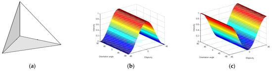
Figure 2.
(a) Trihedral, (b) co-pol and (c) cross-pol polarimetric signatures characterizing scattering.
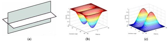
Figure 3.
(a) Dihedral, (b) co-pol and (c) cross-pol polarimetric signatures characterizing scattering.
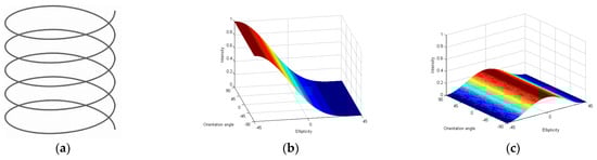
Figure 4.
(a) Left helix, (b) co-pol and (c) cross-pol polarimetric signatures characterizing scattering.
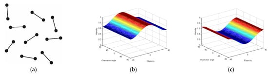
Figure 5.
(a) Cloud of randomly oriented dipoles, (b) co-pol and (c) cross-pol polarimetric signatures characterizing scattering.
As can be seen in Figure 2, Figure 3, Figure 4 and Figure 5, the polarimetric signatures of different scattering types differ in one or even in both polarimetric channels. Those differences can be used to distinguish these scattering mechanisms and, consequently, to categorize objects that are represented by those signatures.
Despite the fact that polarimetric signatures were originally developed as a tool for visual inspection of polarimetric properties of the scatterers, they have found numerous applications in the advanced processing and interpretation of polarimetric SAR data. In [23,24], polarimetric signatures were used for identification of coherent scatterers. Jafari et al. [11] exploited signatures for land-cover classification. In turn, Nunziata et al. [17] revealed a potential application of polarimetric signatures in oil-slick observation.
2.3. Polarimetric Signature-Based Decomposition
The concept of polarimetric signature-based decomposition proposed in this work is established based on the fact that the observed signature (calculated for a pixel of an SAR image) is actually a sum of polarimetric signatures of all objects located within the area represented in this pixel. It leads to the formula (Equation (7)). The observed signature (σobs) can be expressed as a weighted sum of polarimetric signatures of canonical objects (σcan) that represent basic scattering-mechanism types.
In Equation (7), Ns denotes the number of scattering mechanisms that are included in the analysis, and βi represent the weighting factor (i.e., amount) of particular scattering mechanism in the observed signature. Originally, all polarimetric signatures (σobs and σcan) have the size of 180 × 90. However, in order to accelerate the computations, they were resized to the 18 × 9 matrix, which fully preserves all the information contained in the original form but allows for a reduction in the computational time. The reduction of the polarimetric signature was done using Matlab function imresize with the nearest-neighbour interpolation method. Afterwards, this matrix was reshaped to the vertical vector (162 × 1). Equation (7) can be rewritten in a matrix form as Equation (8):
where A is a rectangular matrix with consecutive canonical [σcan_1, σcan_2, ..., σcan_N] columns. In this approach, it is assumed that the weighting factors saved in vector β sum up to 1 and that they have nonnegative values. This last requirement is necessary to avoid the problem described in [25] related to the nonphysical results of some decomposition procedures showing negative powers. A solution based on Matlab function lsqnonneg was used in order to enforce the non-negative results.
Aβ = σobs
3. Polarimetric Signature-Based Decomposition Using SIRT and Simulated Annealing Methods
Systems of linear equations, as in Equation (8), can be solved using several methods. If matrix A is well-conditioned, the matrix-decomposition method can be used to obtain the value of vector β (i.e., LU or SVD decompositions). When significant noise is present or A is a sparse matrix, iterative methods can provide a more stable solution. In real polarimetric signatures, noise is usually present; therefore, iterative methods can be beneficial. Moreover, those methods are more flexible in the implementation of a boundary condition for the solution.
Iterative methods in every step calculate corrections, which are added to the previous solution. There are two approaches to obtain those corrections: deterministic (i.e., conjugate gradients, ART/SIRT methods) or random (i.e., Metropolis algorithm, simulated annealing, genetic algorithms). In both cases, calculations are stopped when a number of iterations reach an assumed level or a value of an evaluation function is less than the assumed threshold.
In this work, two methods were adopted to solve the given system of linear equations (Equation (8)): simulated annealing and SIRT (simultaneous iterative reconstruction technique). Simulated annealing [26] is a probabilistic technique used for approximation of the global optimum of a given function in a large search space. It has found numerous applications in remote sensing [21,27,28] and in computational geosciences [29,30] but not yet in the polarimetric decomposition problem. The SIRT [31] is a very suitable technique for inverting large, sparse linear systems since it is iterative and does not need the whole matrix to be stored in the internal computer memory. It was designed for medical tomography but is nowadays used in different applications. However, up to now, its utilization in remote sensing has been limited. Both selected methods are effective for multidimensional optimization [32,33].
The main aim of application of the selected methods in polarimetric decomposition is to find the vector, β, which minimizes the evaluation function given by Equation (9).
where T denotes transposition, and length() is a length of vector .
The maximum number of iterations was chosen as a stop condition for both algorithms. An equal number of algorithm iterations for all pixels of a polarimetric image caused almost equal time of calculations for each pixel. This assumption makes parallelization of the algorithm easier to implement and more effective.
The SIRT algorithm, in each iteration, calculates corrections of vector Δβj and adds it to the current solution. This vector is calculated using Equation (10) [34].
where Ai,: is the i-th row of matrix A and w is the vector of weights of the same length as β, which contains the number of non-zero elements in the corresponding column of matrix A.
The simulated annealing algorithm uses a probabilistic method to update the current solution. In each iteration, first, vector of corrections is drawn from normal distribution with mean equal to zero and a given standard deviation (std) and is then added to the previous solution. If the new solution has better evaluation than previous one, the new solution is accepted. In the case of a worse evaluation function value, the probability of acceptance is calculated using the Boltzmann distribution given in Equation (11).
where:
- best_eval—the best value of evaluation function β obtained during calculation;
- eval—value of evaluation function for current solution β;
- Tem—temperature, decreases in each iteration: Temi+1= Temi/dt (where dt > 1, usually close to 1).
During iterations, temperature decreases and probability of acceptance of a worse solution also decreases. Acceptance of worse solution is necessary to abandon local minimum. The solution with the lowest value of evaluation function during the whole calculation is returned as a final result.
In both approaches—simulated annealing and SIRT—no constant background level was included as an additional component in the polarimetric signature. Polarimetric signatures can be characterized by a pedestal that arises when multiple scattering mechanisms occur in a given pixel. However, this effect was not included directly in the recognition in order to preserve the algorithm’s capacity to distinguish between single-bounce and volume-scattering signatures, which are similar but differ by the pedestal in the volume-scattering signature.
4. Validation of the Proposed SA- and SIRT-Based Decompositions Using Synthetic Data
Application and validation of the proposed SA- and SIRT-based polarimetric decompositions were performed both for synthetic data and real quad-pol SAR data acquired from TerraSAR-X satellite. After that, the results of the more effective method were compared with the outcomes of Arii decomposition, as well as with the optical image of the studied region.
In both the proposed SA- and SIRT-based decomposition procedures, four scattering mechanisms were taken into consideration: single-bounce (SB), double-bounce (DB), helix scattering (HX) and volume scattering (VOL). In such cases Equation (7) takes the form of (Equation (12)).
For each of the included scattering mechanisms, the polarimetric signatures were calculated using appropriate models. The volume-scattering mechanism was modelled using a cloud of randomly oriented dipoles.
4.1. Validation of the SA- and SIRT-Based Decompositions for Synthetic Signatures without and with Added Noise
In the first step, the SA- and SIRT-based polarimetric decompositions were tested for recognition of synthetic signatures of selected canonical objects. The tests were performed for synthetic signatures without (σn0) and with added noise (σn1, σn2). Two kinds of noise were considered: white (n1) and (n2) colored. The level of noise, for both cases, was set at 19 dB, which corresponds to the noise level of TerraSAR-X satellite [35]. The amounts, βi, of each scattering mechanism in recognized signatures were determined and saved in precents.
The results of SA-based decomposition for recognition of synthetic polarimetric signatures are gathered in Table 1.

Table 1.
Results of SA-based decomposition for synthetic polarimetric signatures (co- and cross-polarized channels). Recognized signatures are specified in percentage.
From Table 1, it can be seen that the SA-based method recognizes the synthetic polarimetric signatures very well without added noise. For this case, all signatures, both in co- and cross-polarized channels, were recognized precisely. Good results were also obtained for synthetic polarimetric signatures with added white noise. However, the in co-polarized channel, noised signature of SB was recognized as a combination of SB and HX polarimetric signatures. Additionally, the noised helix signature was recognized as a combination of DB and HX signatures. Nonetheless, it has to be noted that for both mentioned noised signatures, the proper component was recognized as dominant. The worst results were obtained in case of σn1_VOL. This signature was recognized with high error in the case of the co-polarized channel and almost completely wrong in the case of the cross-polarized channel. The SA-based decomposition method derived very good results in recognition in the cross-polarized channels, as well as for the synthetic signatures with added colored noise. Small imprecision occurred only for noised signatures of helix and volume scattering. In the co-polarized channel, the worst results were obtained for σn2_VOL. For this case, the volume scattering was mistakenly identified as a combination of all scattering mechanisms, with domination of SB and DB.
In Table 2, the results obtained for recognition of synthetic signatures using the SA-based decomposition method are summarized in the context of revealed inaccuracies. For each considered synthetic signature, the average difference, understood as an error, between the expected and calculated amount of the scattering mechanism were determined. These errors were calculated separately for the co-pol channel (εco) and cross-pol channel (εcross). Additionally, for each group of tested data (σn0, σn1, σn2), the average errors of recognition were determined () for both polarimetric channels.
Table 2.
Inaccuracies for SA-based decomposition method revealed for synthetic-signature recognition. Recognized signatures are specified in percentage.
It can be seen in Table 2 that SA-based recognition of synthetic signatures without added noise is not burdened by any error. In the case of signatures with added white noise, the worst results were obtained for the noised volume-scattering signature, where the average difference between expected and obtained percentage of scattering components was equal 23% for the co-pol channel and 43% for the cross-pol channel. In the case of signatures with colored noise, the worst results were obtained for the co-pol channel for σn0_VOL, where the inaccuracy of recognition is at a level of 41%. However, for the cross-polarized channel, the average inaccuracy of all signature recognition is very low, equal to 1.5%.
In Table 3, the results of SIRT-based decomposition for synthetic polarimetric signatures are gathered.
Table 3.
Results of SIRT-based decomposition for synthetic polarimetric signatures (co- and cross-polarized channels). Recognized signatures are specified in percentage.
The results presented in Table 3 reveal that the SIRT-based method derived worse results in recognition of signatures without noise than the SA-based method. For the cross-pol channel, the SIRT method incorrectly identifies σn0_VOL as a combination of all considered scattering mechanisms. Problems also occur in the case of the co-pol channel and signatures with added white noise. Those signatures are recognized with high error, especially for σn1_VOL and σn1_DB. For the cross-pol channel, the results are better. However, the noised signature of volume scattering is recognized as a signature of the SB mechanism. The results for signatures with colored noise are better for the co-pol channel than in the case of signatures with white noise and are exactly the same for the cross-pol channel. The values presented in Table 4, analogous to those in Table 2, summarize the results of the SIRT-based method for synthetic signature recognition in the context of revealed inaccuracies.
Table 4.
Inaccuracies for the SIRT-based decomposition method revealed for synthetic signature recognition. Recognized signatures are specified in percentage.
Comparing average values presented in Table 2 and Table 4, it can be seen that the SIRT-based method provides less accurate results of synthetic signature recognition than the SA-based method. For the SIRT-based method, the most significant problems occur in the case of σn0_VOL recognition. What is more, the results for recognition of synthetic signatures with white noise are also not very accurate, especially for the co-pol channel, for which = 20.49%.
4.2. Validation of the SA- and SIRT-Based Decomposition Methods for Linear Combinations of Synthetic Signatures
In this step, the proposed SA- and SIRT-based methods were tested for decomposition of linear combinations of canonical polarimetric signatures. In order to do that, eight polarimetric signatures were prepared (σ1−σ8). Each of them was generated as a linear combination of polarimetric signatures of selected canonical objects representing considered scattering mechanisms (Table 5). For each of them, the decomposition was applied separately for the co- and cross-polarized channel. Like in the previous section, the amount (βi) of a particular scattering mechanism in a considered signature was determined and saved as a percentage of recognized polarimetric signatures. The results obtained for SA-based decomposition are gathered in Table 5.
Table 5.
Results of SA-based decomposition for linear combinations of synthetic signatures (co- and cross-polarized channels). Recognized signatures are specified in percentage.
The obtained results reveal that the simulated annealing method works well in the recognition of the amount of polarimetric signatures in the linear combination of them. For the co-polarized channel, the proposed method properly recognized the amount of polarimetric signatures in all studied examples. In the cross-polarized channel, the results of the SA-based method are less accurate. In the cross-pol channel, the helix scattering mechanism is mistaken with the scattering mechanism of the volume horizontal model. The worst results were obtained for the cross-pol channel for the linear combination (σ6) of volume and helix scattering. In this case, the algorithm underestimated those mechanisms and improperly recognized a double-bounce scattering mechanism.
The SIRT-based decomposition results obtained for a linear combination of signatures are presented in Table 6.
Table 6.
Results of SIRT-based decomposition for linear combinations of synthetic signatures (co- and cross-polarized channels). Recognized signatures are specified in percentage.
Analysis of the obtained results reveals that the proposed SIRT-based method recognizes linear combination of polarimetric signatures very well. The accuracy is very high, especially for the co-polarized channel, where tested synthetic data were properly recognized in 100% of instances. The results obtained for cross-polarized channel are less accurate but still promising. For the cross-polarized channel, from eight analyzed linear combinations of polarimetric signatures, five of them were correctly recognized. The worst results were obtained for σ2 and σ4.
In Table 7, the values of error revealed for SA- and SIRT-based methods in recognition of linear combinations of signatures are compared.
Table 7.
Inaccuracies for SA- and SIRT-based decompositions revealed for linear combinations of polarimetric signatures. Recognized signatures are specified in percentage.
Analysis of the values presented in Table 7 reveal that for the co-polarized channel, both SA- and SIRT-based methods precisely recognized all tested combinations of polarimetric signatures. However for the cross-pol channel, the results obtained using the SIRT-based method are almost two times better than those obtained using the SA-based method. The most significant differences in accuracy of the results occur in the case of σ2, σ3 and σ6.
4.3. Validation of the SA- and SIRT-Based Polarimetric Decompositions Results for Real SAR Data
Validation of the SA- and SIRT-based polarimetric decomposition results was also performed for real satellite SAR data gathered by TerraSAR-X satellite. The radar image used for this purpose covers the area the town of Mahlow, located south of Berlin. The spatial resolution of the image is 1.7 m × 6.5 m. The Pauli color composition map of polarimetric channels and the optical image of the studied region are presented in Figure 6.
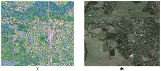
Figure 6.
(a): Pauli-coded color composition of polarimetric channels (red: |hh-vv|, green: |hv|, blue: |hh+vv|). (b): optical image of studied region (source: Google Earth).
As can be seen in Figure 6a, different terrain types are present in the studied region, which is advantageous for the validation process. Part of the region is covered by built-up areas. There are also agricultural fields with bare soil and low vegetation, as well as some forested areas.
In order to perform the test for real data, the pixels that best represent four considered scattering mechanisms were selected from the analyzed image. The selection was done based on the Yamaguchi decomposition and mean alpha angle (α) from H/A/alpha decomposition. Both mentioned decompositions belong to the most widely used methods of SAR image processing since they are characterized by relatively high accuracy. Based on the four-component Yamaguchi decomposition [7], the values of four scattering mechanisms (SB, DB, HX, VOL) in each pixel can be estimated. To model volume scattering, Yamaguchi exploits three models, which are selected based on (Equation (13)).
If the ratio is smaller than −2 dB, the volume scattering is modelled by a cloud of randomly oriented, very thin, horizontal cylinder-like scatterers. For μ between −2 dB and 2 dB, the volume scattering is represented by a cloud of randomly oriented dipoles with a uniform probability function for the orientation angle [4]. If the μ is higher than 2 dB, a cloud of randomly oriented, very thin, vertical cylinder-like scatterers is used as a model.
In this work, in order to select appropriate real signatures, the power of each scattering mechanism recognized using Yamaguchi decomposition was divided by the sum of powers of all scattering mechanisms in a given pixel. This gave the relative power (Prel) of all scattering mechanisms in all pixels. The pixels for which this relative power was the highest were selected as a representative. Since none of the decompositions provide unambiguous results and there are always some errors in the outcomes, the selection of representative pixels was additionally strengthened by use of mean alpha angle from H/A/alpha decomposition. The values of this parameter are related to three scattering mechanisms (SB, DB, VOL). Values of σ between 0° and approximately 40° are characteristic for surface scattering, values between 40° and 50° occur in the case of volume diffusion and the values between 50° and 90° correspond to a double-bounce scattering mechanism. The alpha angle does not provide information about the helix scattering mechanism; therefore, identification of this mechanism suffers from the occurrence of the greatest error. The thresholds for both parameters (Yamaguchi decomposition parameters and alpha angle) are given in Table 8.
Table 8.
Thresholds for the Yamaguchi parameters and alpha angle.
The obtained results of the validation procedure of SA-based decomposition are gathered in Table 9. Each row presents the averaged accuracies for all selected pixels dominated by each scattering mechanism.
Table 9.
Results of SA-based decomposition for real data (co- and cross-polarized channels). Recognized signatures are specified in percentage.
The obtained results reveal that the proposed simulated annealing method derives promising results. Its accuracy is very high in recognizing real polarimetric signatures of trihedral and dihedral (in both co- and cross-polarized channels). Good results were also obtained in the co-polarized channel in recognizing real polarimetric signatures of helix. The results of the SA-based method in recognizing real polarimetric signatures of volume scattering are not so clear. However, since the chosen real signatures cannot be treated as a pure representation of considered mechanisms, especially in case of helix and volume scattering, the obtained outcomes are not surprising. The discrepancies can also be associated with the models that were used in the proposed polarimetric signature-based solution and in Yamaguchi decomposition to represent volume scattering.
The validation results obtained for SIRT-based decomposition applied to real SAR data are presented in Table 10.
Table 10.
Results of SIRT-based decomposition for real data (co- and cross-polarized channels). Recognized signatures are specified in percentage.
The results obtained using the SIRT method are very similar to those obtained using the simulated annealing approach. The worst results were obtained for real signatures of helix and volume scattering. However, for those cases, slightly better outcomes were obtained in the case of the SIRT method.
In Table 11, the values of error revealed for SA- and SIRT-based methods in recognition of real polarimetric signatures are compared.
Table 11.
Inaccuracies for SA- and SIRT-based decompositions for real polarimetric signatures. Recognized signatures are specified in percentage.
It can be seen in Table 11 that for the co-polarized channel, both considered methods are characterized by inaccuracies in almost the same way (about 18%). However, for the cross-polarized channel, the SIRT-based decomposition method works slightly better in recognition of real polarimetric signatures. The improvement relates mainly to σVOL recognition.
To facilitate easier comparison of SA- and SIRT-based methods, the values from Table 2, Table 4, Table 7 and Table 11 are gathered in Table 12.
Table 12.
Values of average errors for SA- and SIRT-based methods for each tested data set. Recognized signatures are specified in percentage.
It can be seen in Table 12 that in the recognition of synthetic signatures of canonical objects, the SA-based method derived better or almost the same results as the SIRT-based approach. For tests performed for linear combinations of signatures, the SA-based method in the cross-pol channel gave worse results than the SIRT method. In turn, the accuracy of real signature recognition is almost the same for both tested approaches. However, taking into account only the co-polarized channel, it can be stated that SA-based decomposition allows for attainment of more accurate results. Therefore, this method and the co-polarized channel were chosen for further testing.
5. GPU Processing
Application of polarimetric signatures in the decomposition procedure is associated with the long computational time of this procedure. This is not a desirable effect. In order to ensure reasonable computational time of the proposed decomposition, processing was performed using graphic processing units (GPU). This approach delivers the possibility of significantly increasing computation speed; however, it requires more programming skill.
Graphic processing units are built using different architecture than in the case of regular computing processing units (CPU). GPUs consist of multiple arithmetic-logic units (ALU), while CPUs are usually built using four cores nowadays. Graphic memory is reorganized and logically portioned to provide for better utilization. Despite pointed advantages, from the programmer’s point of view, GPU units are more difficult to use. They require knowledge of a specific language (like CUDA or OpenCL) and compliance with a sophisticated multithreaded approach. The programmer writes two codes: the first is responsible for CPU-GPU communications and is called the host code (as it is executed by host machine, a CPU), and the second is executed in a function called a “kernel” on the GPU (referred as “device”).
In this work, CUDA language was chosen to increase computation speed of the proposed decomposition using GPU. The main requirement was to use an NVidia graphic card, the only hardware capable of using CUDA. Programs were compiled using CUDA 6.5 [36].
The simulated annealing algorithm is based on the synchronous solution presented in [37]. However, the “synchronous” part was also moved to the kernel, which will be explained later. This solution was chosen because it prevents the operating system from rising watchdog limit and terminating long CUDA kernel executions (the program was extended with real-time results visualization, so display context was required). Moreover, Ferreiro et al. [37] noticed smaller errors using this approach.
Simulated annealing in the parallel approach starts with random coefficient initialization in vector β0. The kernel, running in hundreds of threads in parallel, evaluates one value of that vector per thread and, using evaluation formula, adjusts it in several steps. The results and the error are stored for further calculation. Then, using reduction on the GPU, the best result (smallest error) is searched for, and the outcome is set as a new input vector for the kernel. Then, the host loop performs the next kernel call, and the process repeats.
In CUDA, every kernel call is asynchronous. The Ferreiro et al. [37] approach required synchronization before reduction and temperature change because it was performed on the host. The proposed method does not require synchronization until the last copying of results. Reduction and temperature change were moved into the GPU.
What is more, to utilize the GPU more efficiently, texture memory was used. It might be considerably faster because of the caching algorithm. Additionally, the values that are known to be constant for whole execution of the program are kept in the GPU’s constant memory.
Another significant improvement of the algorithm is the application of CUDA streams. This technique allows the user to run multiple streams of command calls in parallel, hence providing more results in a similar time [38]. In this application, the streams are used to simultaneously calculate multiple values.
Listing 1.
Simulated annealing host pseudocode.
Listing 1.
Simulated annealing host pseudocode.
| Allocation of memory and textures |
| Random vector initialization (GPU) |
| Constant memory population |
| for desired number of steps do { |
| for each stream{ |
| kernel_SA |
| } |
| for each stream{ |
| kernel_reduction |
| } |
| } |
| Copy results to host |
Listing 2.
Simulated annealing kernel.
Listing 2.
Simulated annealing kernel.
| Select new best point as a starting point |
| Adjust temperature |
| Evaluation |
| for desired number of steps{ |
| New random point |
| Evaluation |
| Update point if better |
| } |
| Save result |
6. SA-Based Decomposition of Real SAR Images
The SA-based method, selected in the previous section the better model, was applied for decomposition of the whole SAR image presented in Figure 6. The resulting images presenting the scattering power of a particular scattering mechanism in each pixel are presented in Figure 7. In order to facilitate the interpretation of the results, the powers of double-bounce and helix scattering mechanisms are summed and presented in one image (Figure 7). Both mechanisms occur in the case of man-made objects usually located within urban areas.
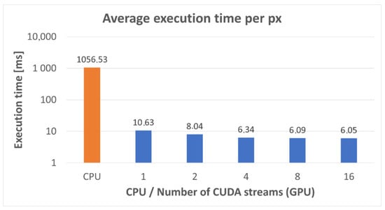
Figure 7.
Average execution times of the SA procedure using CPU and GPU with different numbers of streams.
Decomposition is executed with the following input parameters for simulated annealing and CUDA configuration of kernels and loop iterations. The simulated annealing parameters were set to: T0 = 1000.0, dt = 1.0025, standard deviation std = 0.005 and maximum number of iterations = 500,000. The search space for all the elements of vector β was set to 0–1000.
Comparison of the execution times on CPU and GPU was possible by adjusting the number of iterations to the parallel environment of the GPU. Therefore, the number of iterations performed on the CPU differs from the number of iterations of kernel execution on the GPU. The calculations are performed in parallel (number of threads are multiplied by number of blocks created), and every kernel evaluates the equation in loop, several times. Hence, the number of kernel calls is significantly lower than the number of iterations in the CPU version of the algorithm. For example, executing a CPU version of the algorithm in 500,000 steps would be equivalent to about 20 calls of CUDA kernels, running in 128 threads on 32 blocks, with six iterations in each kernel. Average execution times of the SA procedure measured for a single pixel performed using CPU and GPU are presented in Figure 7.
The results of the proposed SA-based polarimetric decomposition method were compared to those obtained using Arii decomposition (Figure 8). Arii et al. [9] extend the idea of model-based decompositions by creating an adaptive decomposition technique, allowing for estimation of both the mean orientation angle and a degree of randomness for the canopy scattering for each pixel in an image. No scattering-reflection symmetry assumption is required to determine the volume contribution.
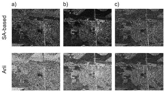
Figure 8.
Results of the proposed SA-based and Arii decomposition: (a) decomposed single-bounce scattering powers, (b) decomposed double-bounce scattering powers, (c) decomposed volume-scattering powers.
In general, the single-bounce mechanism is dominant in the case of surfaces like roads, rivers, lakes, agriculture fields, etc. By comparing the image of power of the single-bounce scattering mechanism obtained using the SA-based method with the corresponding image of Arii decomposition (Figure 8a), it can be concluded that the latter seems to overestimate single-bounce scattering for almost all terrain types. In contrast, the SA-based decomposition shows underestimation of this mechanism within agricultural fields. Both methods correctly recognized the flat, elongated roofs of garages in the NE part of built-up area. The assessed amount of the double-bounce mechanism, which is characteristic of vertical structures, like walls of buildings, is more plausible in the case of the SA-based method. The structure of the city is visible and very clear. The locations of individual buildings are well recognized. There is no overestimation of double-bounce scattering within agricultural fields and forests, which seems to take place in the case of Arii decomposition results (Figure 8b). Both considered methods deal well with the recognition of buildings that are rotated toward the radar line of sight. The reliability of the volume-scattering identification is higher in the case of the SA-based method (Figure 8c). The power of volume scattering should be the highest for vegetated areas. Arii decomposition significantly overestimates volume-scattering within built-up areas (Figure 8c). This is demonstrated for the NE part of the built-up area, where the highest powers of the volume-scattering mechanism are decomposed for buildings.
Comparison of the decomposition results obtained using Arii and SA-based methods shows that the newly proposed solution has a number of advantages. The most important is the decrease in volume overestimation in the case of urban areas. This results in an easier interpretation of results, especially for areas with buildings rotated around the radar line of sight. In addition, the SA-based method identifies more volume-scattering mechanisms within forests and does not overestimate single- and double-bounce within such regions, as is in the case of Arii decomposition. The disadvantage of the proposed decomposition is some underestimation of single-bounce scattering mechanisms within agriculture fields.
7. Summary and Conclusions
Application of the polarimetric signatures for decomposing the received radar signal into basic scattering mechanisms is a new approach to the polarimetric decomposition problem. The proposed decomposition method provides robust and high-quality results. It was shown that the proposed method does not overestimate the volume-scattering component in built-up areas and clearly separates objects within the mixed-up areas, where both buildings and vegetation surfaces occur.
Two different approaches to the decomposition of polarimetric signatures were tested: simulated annealing and SIRT methods. The simulated annealing algorithm was chosen to search for the optimal solution of decomposition of real polarimetric signature into canonical signatures.
The following answer to the question posed at the beginning can be given. Application of polarimetric signatures, together with iterative methods for solving the system of linear equations in decomposition, can provide additional information about the studied area. Despite the fact that polarimetric signatures are calculated based on a scattering matrix and, theoretically, do not contain additional information, their utilization in decomposition can be beneficial.
The proposed approach was very time-consuming; therefore, it was parallelized using CUDA technology to be executed on graphical processing units. A special simulated annealing algorithm was designed for execution on GPU. This resulted in a speeding up of 175 times compared to the regular CPU version. However, the time of the decomposition of the 1500 × 1500 pixel a SAR image is still relatively long, which will require further developments either of the decomposition algorithm itself or of its parallelized version.
Author Contributions
Conceptualization, S.P.-S., J.S., K.S., M.D. and A.L.; methodology, S.P.-S., J.S., K.S., M.D. and A.L.; software, S.P.-S., K.S. and M.D.; validation S.P.-S., J.S., K.S., M.D. and A.L.; formal analysis S.P.-S., J.S., K.S., M.D. and A.L.; investigation, S.P.-S., J.S., K.S., M.D., A.L., J.B. and A.F.; resources, S.P.-S. and J.S.; data curation, M.D., A.F. and J.B.; writing—original draft preparation, A.F.; writing—review and editing, S.P.-S., J.B. and A.F.; visualization, S.P.-S., M.D., A.F. and J.B.; supervision, J.B. and A.F.; project administration, A.F. and J.B.; funding acquisition, S.P.-S., M.D., A.F. and J.B. All authors have read and agreed to the published version of the manuscript.
Funding
This work was financed by ESA within the framework of the project “Pattern recognition-based decomposition method for quad-polarimetric SAR data” and supported by the AGH-University of Science and Technology, Faculty of Geology, Geophysics and Environmental Protection, as a part of a statutory project. TerraSAR-X data used in this research were provided by DLRwork.
Institutional Review Board Statement
Not applicable.
Informed Consent Statement
Not applicable.
Data Availability Statement
The data can be accessed upon request from any of the authors.
Conflicts of Interest
The authors declare no conflict of interest.
References
- Oliver, C.; Quegan, S. Understanding Synthetic Aperture Radar Images; SciTechPublishing: Boston, MA, USA, 2004. [Google Scholar]
- Gupta, R.P. Remote Sensing Geology; Springer: Berlin, Germany, 2017. [Google Scholar]
- Ferretti, A.; Prati, C.; Rocca, F. Permanent Scatterers in SAR Interferometry. IEEE Trans. Geosci. Remote Sens. 2001, 39, 8–20. [Google Scholar] [CrossRef]
- Lee, J.S.; Pottier, E. Polarimetric Radar Imaging: From Basic to Applications; CRC Press, Taylor & Francis Group: Boca Raton, FL, USA, 2009. [Google Scholar]
- Cloude, S.R.; Pottier, E. A review of target decomposition theorems in radar polarimetry. IEEE Trans. Geosci. Remote Sens. 1996, 34, 498–518. [Google Scholar] [CrossRef]
- Freeman, A.; Durden, S.L. A three-component scattering model for polarimetric SAR data. IEEE Trans. Geosci. Remote Sens. 1998, 36, 963–973. [Google Scholar] [CrossRef]
- Yamaguchi, Y.; Moriyama, T.; Ishido, M.; Yamada, H. Four-component scattering model for polarimetric SAR image decomposition. IEEE Trans. Geosci. Remote Sens. 2005, 43, 1699–1706. [Google Scholar] [CrossRef]
- Touzi, R. Target scattering decomposition in terms of roll-invariant target parameters. IEEE Trans. Geosci. Remote Sens. 2007, 45, 73–84. [Google Scholar] [CrossRef]
- Arii, M.; van Zyl, J.J.; Kim, Y. Adaptive model-based decomposition of polarimetric SAR covariance matrices. IEEE Trans. Geosci. Remote Sens. 2011, 49, 1104–1113. [Google Scholar] [CrossRef]
- van Zyl, J.J.; Zebker, H.A.; Elachi, C. Imaging radar polarization signatures: Theory and observation. Radio Sci. 1987, 22, 529–543. [Google Scholar] [CrossRef]
- Jafari, M.; Maghsoudi, Y.; Zoej, M.J.V. A new method for land cover characterization and classification of polarimetric SAR data using polarimetric signatures. IEEE J. Sel. Top. Appl. Earth Obs. Remote Sens. 2015, 8, 3595–3607. [Google Scholar] [CrossRef]
- Zeller, C. Cuda C/C++ Basics; NVIDIA Coporation: Santa Clara, CA, USA, 2011. [Google Scholar]
- Mattia, F.; Le Toan, T.; Souyris, J.-C.; de Carolis, G. The Effect of Surface Roughness on Multifrequency Polarimetric SAR Data. IEEE Trans. Geosci. Remote Sens. 1997, 35, 954–966. [Google Scholar] [CrossRef]
- Ballester-Berman, J.D.; Vicente-Guijalba, F.; Lopez-Sanchez, J.M. Polarimetric SAR Model for Soil Moisture Estimation over Vineyards at C-band. Prog. Electromagn. Res. 2013, 142, 639–665. [Google Scholar] [CrossRef]
- Zhang, B.; Perrie, W.; Vachon, P.W.; Xiaofeng, L.; Pichel, W.G.; Jie, G.; Yijun, H. Ocean Vector Winds Retrieval From C-Band Fully Polarimetric SAR Measurements. IEEE Trans. Geosci. Remote Sens. 2012, 50, 4252–4261. [Google Scholar] [CrossRef]
- Praks, J.; Hallikainen, M.; Antropov, O.; Molina-Hurtado, D. Boreal Forest Tree Height Estimation from Interferometric Tandem-X Images. In Proceedings of the IEEE International Geoscience and Remote Sensing Symposium (IGARSS 2012), Munich, Germany, 20–27 July 2012. [Google Scholar]
- Nunziata, F.; Migliaccio, M.; Gambardella, A. Pedestal height for sea oil slick observation. IET Radar Sonar Navigat. 2011, 5, 103–110. [Google Scholar] [CrossRef]
- Goodenough, D.G.; Chen, H.; Richardsonm, A.; Cloude, S.; Hong, W.; Li, Y. Mapping Fire Scars Using Radarsat-2 Polarimetric SAR data. Can. J. Remote Sens. 2011, 37, 500–509. [Google Scholar] [CrossRef]
- Alberga, V.; Krogager, E.; Chandra, M.; Wanielik, G. Potential of coherent decompositions in SAR polarimetry and interferometry. In Proceedings of the IEEE International Geoscience and Remote Sensing Symposium IGARSS ’04, Anchorage, AK, USA, 20–24 September 2004; Volume 3. [Google Scholar]
- Chen, S.-C.; Ohki, M.; Shimada, M.; Sato, M. Deorientation Effect Investigation for Model-Based Decomposition Over Oriented Built-Up Areas. IEEE Geosci. Remote Sens. Lett. 2012, 10, 273–277. [Google Scholar] [CrossRef]
- Hong, S.-H.; Wdowinski, S. Double-bounce component in cross-polarimetric SAR from a new scattering target decomposition. IEEE Trans. Geosci. Remote Sens. 2014, 52, 3039–3051. [Google Scholar] [CrossRef]
- Yang, W.; Song, H.; Xia, G.-S.; Xu, X. On the Mixed Scattering Mechanism Analysis of Model-Based Decomposition for Polarimetric SAR Data. Prog. Electromagn. Res. B 2013, 52, 327–345. [Google Scholar] [CrossRef][Green Version]
- Bielecka, M.; Porzycka-Strzelczyk, S.; Strzelczyk, J. SAR images analysis based on polarimetric signatures. Appl. Soft. Comput. 2014, 23, 259–269. [Google Scholar] [CrossRef]
- Strzelczyk, J.; Porzycka-Strzelczyk, S. Identification of coherent scatterers in SAR images based on the analysis of polarimetric signatures. IEEE Geosc. Remote Sens. Lett. 2014, 11, 783–787. [Google Scholar] [CrossRef]
- van Zyl, J.J.; Arii, M.; Kim, Y. Model-based decomposition of polarimetric SAR covariance matrices constrained for nonnegative eigenvalues. IEEE Trans. Geosci. Remote Sens. 2011, 49, 3452–3459. [Google Scholar] [CrossRef]
- Kirkpatrick, S.; Gelatt, C.D.; Vecchi, M.P. Optimization by Simulated Annealing, Science. New Ser. 1983, 220, 671–680. [Google Scholar]
- Chang, Y.-L.; Fang, J.-P. A Simulated Annealing Band Selection Approach for High-Dimensional Remote Sensing Images. In Simulated Annealing, Theory with Applications; Chibante, R., Ed.; IntechOpen: London, UK, 2010; Chapter 3. [Google Scholar]
- Liu, D. Simulating remotely sensed imagery for classification evaluation. Int. Arch. Photogramm. Remote Sens. Spat. Inf. Sci. 2008, 37, 299–304. [Google Scholar]
- Bangerth, W.; Klie, H.; Wheeler, M.F.; Stoffa, P.L.; Sen, M.K. On optimization algorithms for the reservoir oil well placement problem. Comp. Geosci. 2006, 10, 303–319. [Google Scholar] [CrossRef]
- Tran, N.H. Simulated annealing technique in discrete fracture network inversion: Optimizing the optimization. Comp. Geosci. 2007, 11, 249–260. [Google Scholar] [CrossRef]
- Gilbert, P. Iterative methods for the 3D reconstruction of an object from projections. J. Theor. Biol. 1972, 76, 105–117. [Google Scholar] [CrossRef]
- Dwornik, M.; Leśniak, A. Comparison between Inversion Algorithms of Surface Refraction Tomography for Cavities Detection. In Proceedings of the Near Surface 2007—13th EAGE European Meeting of Environmental and Engineering Geophysics, Istanbul, Turkey, 3–5 September 2007. [Google Scholar]
- Velis, D.R. Traveltime inversion for 2-Danomaly structures. Geophysics 2001, 62, 1481–1487. [Google Scholar] [CrossRef][Green Version]
- Lo, T.; Inderwiesen, P.I. Fundamentals of Seismic Tomography. In Geophysical Monograph Series; No.6; Society of Exploration Geophysicist: Tulsa, OK, USA, 1994. [Google Scholar]
- Romeiser, R.; Breit, H.; Eineder, M.; Runge, H.; Flament, P.; de Jong, K.; Vogelzang, J. On the Suitability of TerraSAR-X Split Antenna Mode for Current Measurements by Along-Track Interferometry. In Proceedings of the IGARSS ’03 2003 IEEE International Geoscience and Remote Sensing Symposium, Toulouse, France, 21–25 July 2003; Volume 2, pp. 1320–1322. [Google Scholar]
- NVIDIA. 2014. Available online: https://developer.nvidia.com/cuda-toolkit-65 (accessed on 21 October 2021).
- Ferreiro, A.M.; García, J.A.; López-Salas, J.G.; Vázquez, C. An efficient implementation of parallel simulated annealing algorithm in GPUs. J. Glob. Optim. 2013, 57, 863–890. [Google Scholar] [CrossRef]
- Rennich, S. (NVIDIA), CUDA C/C++ Streams and Concurrency. 2011. Available online: http://on-demand.gputechconf.com/gtc-express/2011/presentations/StreamsAndConcurrencyWebinar.pdf (accessed on 21 October 2021).


Publisher’s Note: MDPI stays neutral with regard to jurisdictional claims in published maps and institutional affiliations. |
© 2021 by the authors. Licensee MDPI, Basel, Switzerland. This article is an open access article distributed under the terms and conditions of the Creative Commons Attribution (CC BY) license (https://creativecommons.org/licenses/by/4.0/).