
A Fractional Step Method to Solve Productivity Model of Horizontal Wells Based on Heterogeneous Structure of Fracture Network

 ,
,
Abstract
:1. Introduction
2. Methodology
2.1. Physical Model
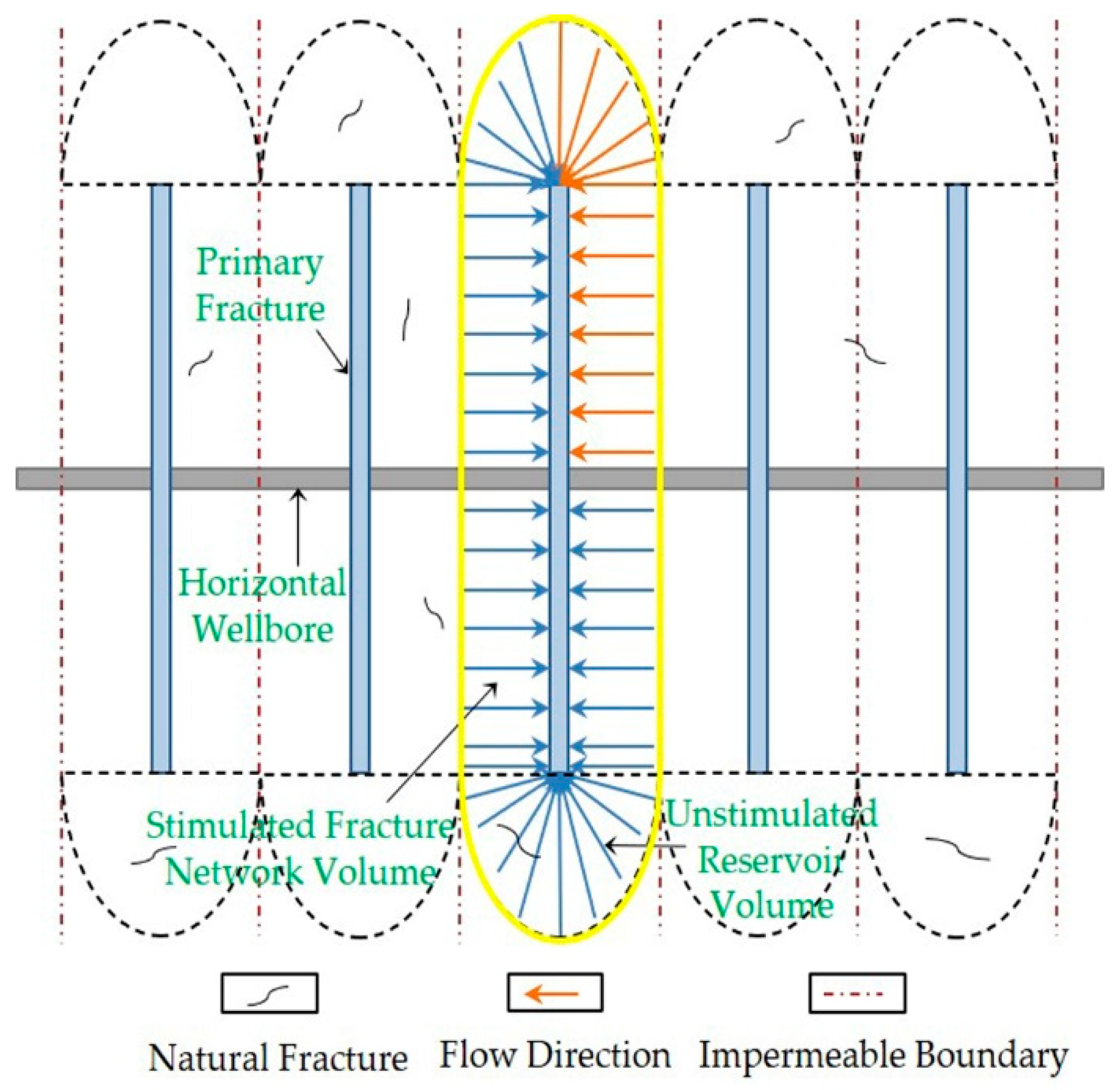
2.1.1. Heterogeneous Fracture Network Structure Model
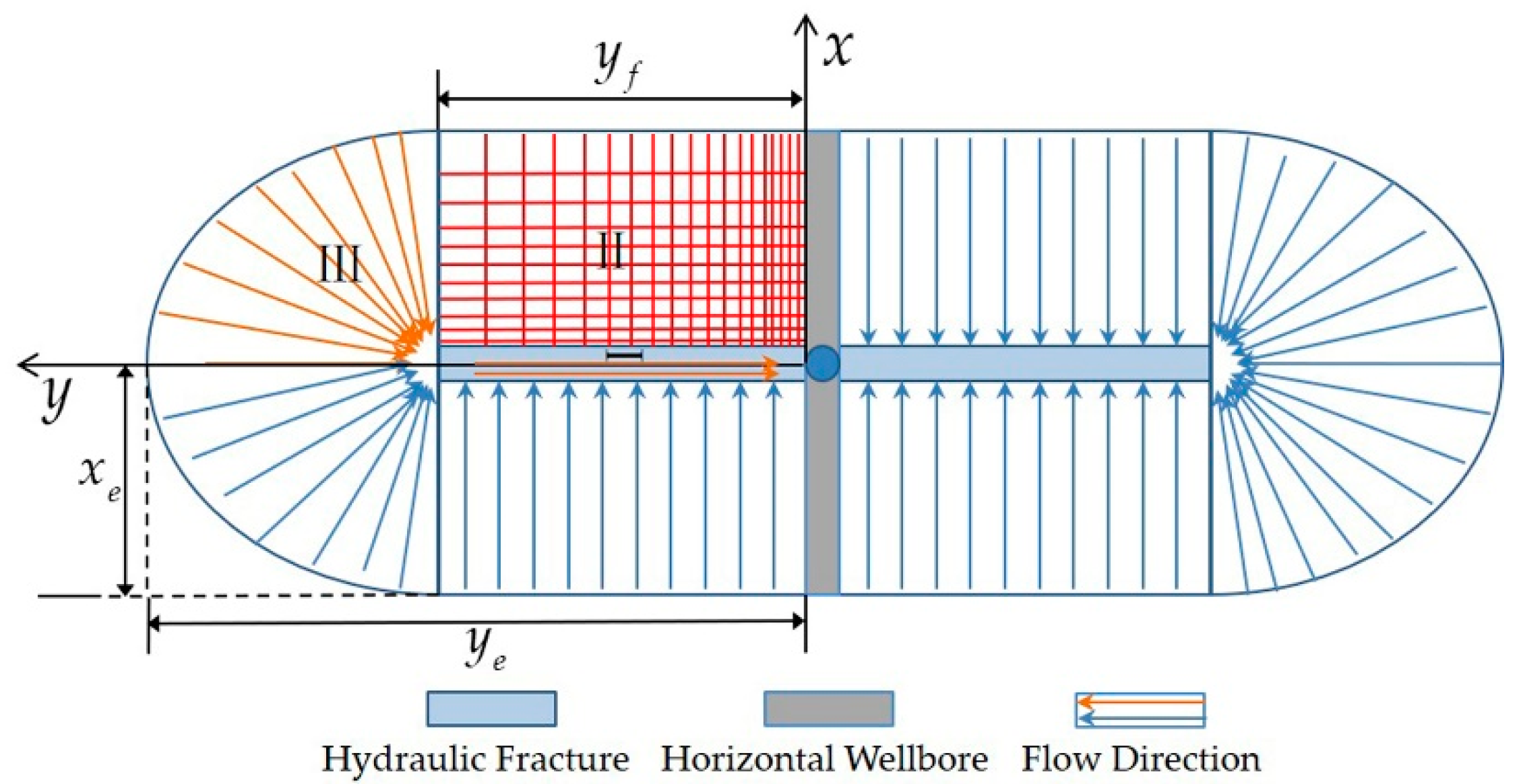
2.1.2. The Steady-State Physical Model of Fractured Horizontal Well
2.2. Mathematical Model and the Solution
2.2.1. Consideration of the Threshold Pressure Gradient
2.2.1.1. Primary Fractures of Infinite Conductivity
- (1)
- Fracture network stimulated volume area (Region II)
- (2)
- Unstimulated volume area at the reservoir boundary (Region III)
- (3)
- Production capacity of horizontal wells
2.2.1.2. Primary Fractures of Finite Conductivity
- (1)
- The primary fracture area (region I)
- (2)
- Fracture network stimulated volume area (Region II)
- (3)
- Unstimulated volume area at the reservoir boundary (Region III)
- (4)
- Production capacity of horizontal wells
2.2.2. Consideration of the Deformation Characteristics of Porous Medium
Primary Fractures of Infinite Conductivity
- (1)
- Fracture network stimulated volume area (Region II)
- (2)
- Unstimulated volume area at the reservoir boundary (Region III)
- (3)
- Production capacity of horizontal wells
Primary Fractures of Finite Conductivity
- (1)
- The primary fracture area (region I)
- (2)
- Fracture network stimulated volume area (Region II)
- (3)
- Unstimulated volume area at the reservoir boundary (Region III)
- (4)
- Production capacity of horizontal wells
2.3. Flow Chart of Established Productivity Model
3. Results and Discussion
3.1. Model Verification
- (1)
- Oilfield examples
- (2)
- Model comparison
3.2. Analysis of Sensitive Factors
- (1)
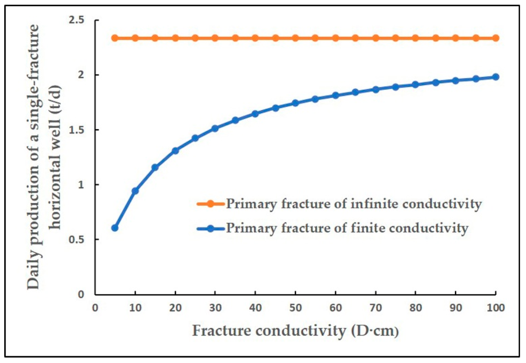
- Fracture conductivity
- (2)
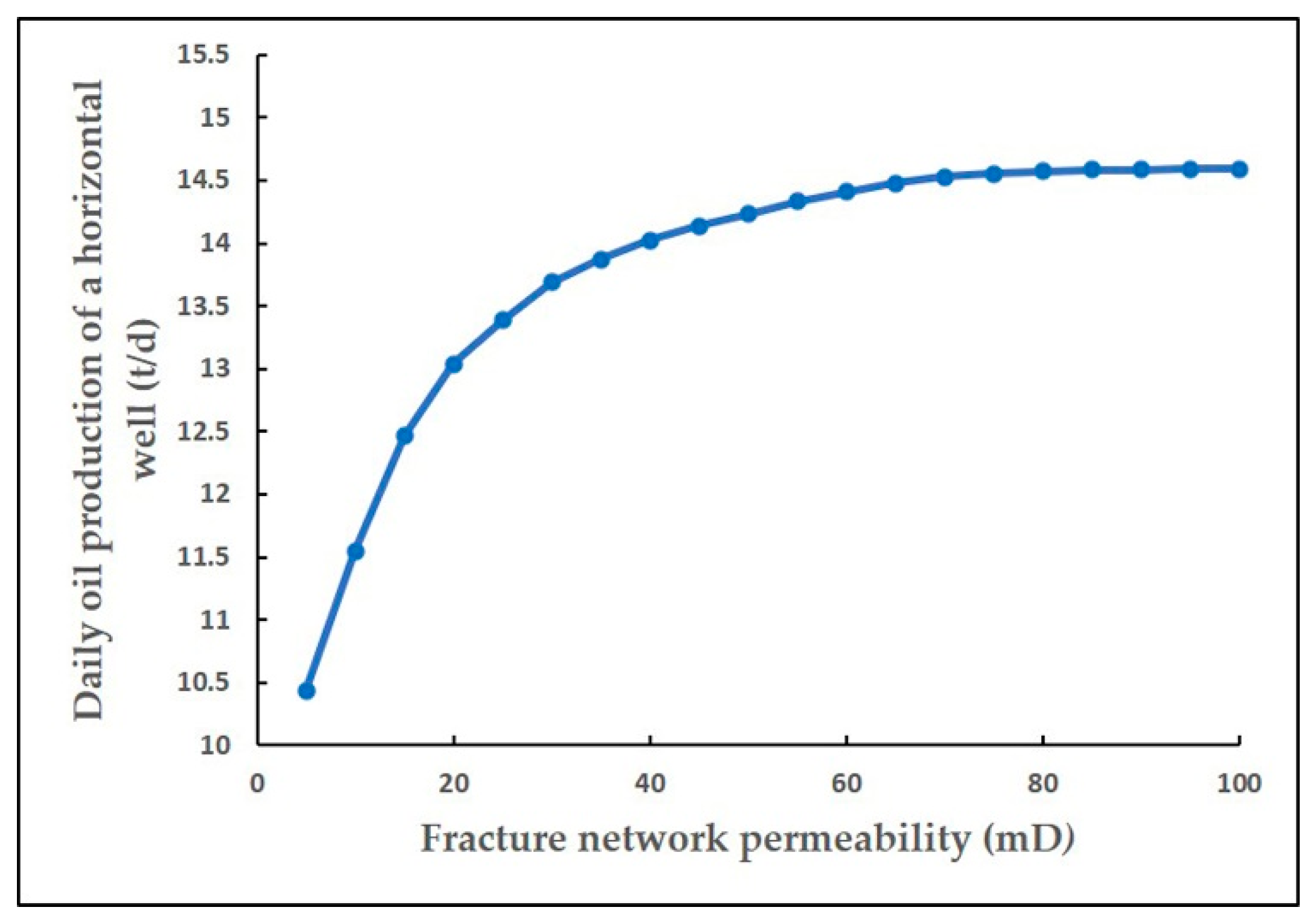
- Fracture network permeability
- (3)
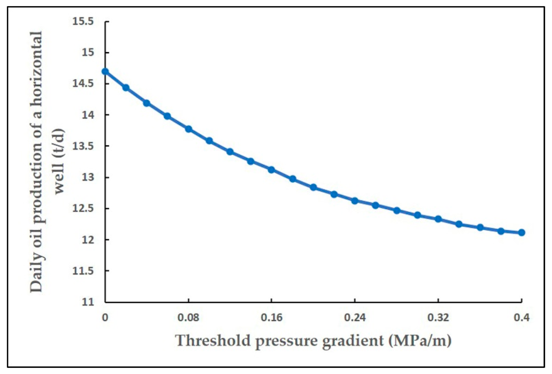
- Threshold pressure gradient
- (4)
- Media deformation coefficient
- (5)
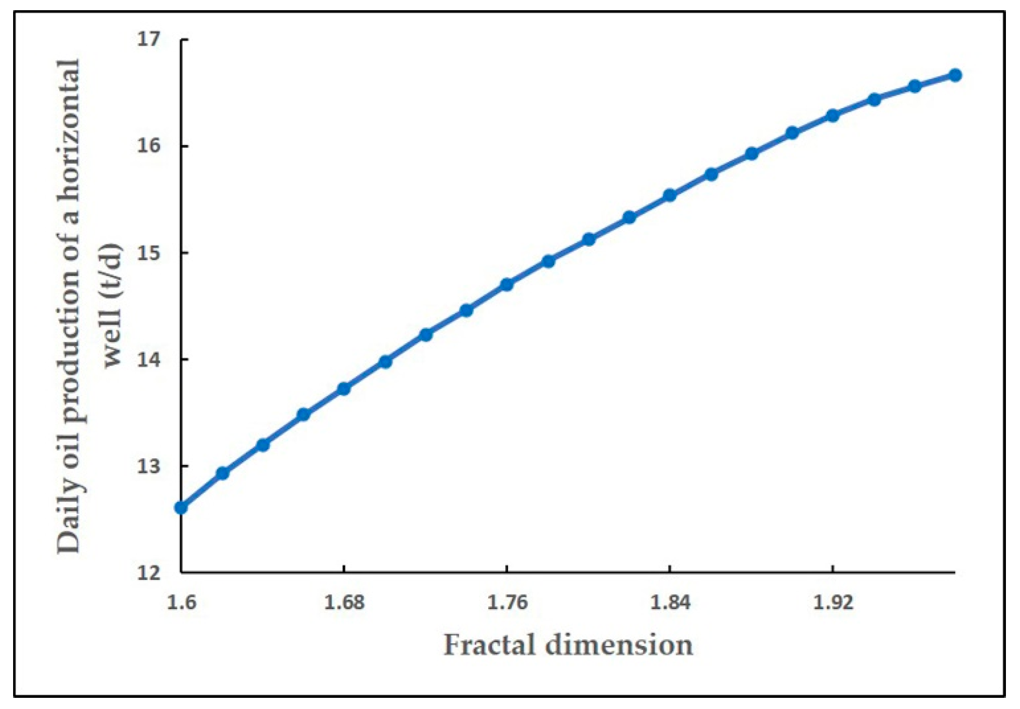
- Fractal dimension
- (6)
- Fracture density within 100 m
4. Conclusions
Author Contributions
Funding
Data Availability Statement
Conflicts of Interest
References
- Liu, H. The numerical simulation for multistage fractured horizontal well in low-permeability reservoirs based on modified Darcy’s equation. J. Pet. Explor. Prod. Technol. 2017, 7, 735–746. [Google Scholar] [CrossRef] [Green Version]
- Fang, W.; Jiang, H.; Li, J.; Wang, Q.; Killough, J.; Li, L.; Peng, Y.; Yang, H. A numerical simulation model for multi-scale flow in tight oil reservoirs. Pet. Explor. Dev. 2017, 44, 446–453. [Google Scholar] [CrossRef]
- Luo, S.; Zhao, Y.; Zhang, L.; Chen, Z.; Zhang, X. Integrated Simulation for Hydraulic Fracturing, Productivity Prediction, and Optimization in Tight Conglomerate Reservoirs. Energy Fuels 2021, 35, 14658–14670. [Google Scholar] [CrossRef]
- Xu, J.; Yang, L.; Liu, Z.; Ding, Y.; Gao, R.; Wang, Z.; Mo, S. A New Approach to Embed Complex Fracture Network in Tight Oil Reservoir and Well Productivity Analysis. Nat. Resour. Res. 2021, 30, 2575–2586. [Google Scholar] [CrossRef]
- Liu, L.; Xiao, Y.; Wu, Z.; Wang, X. Hydro-mechanical coupling numerical simulation method of multi-scale pores and fractures in tight reservoir. IOP Conf. Ser. Earth Environ. Sci. 2022, 983, 012060. [Google Scholar] [CrossRef]
- Ezulike, O.; Igbokoyi, A. Horizontal well pressure transient analysis in anisotropic composite reservoirs—A three dimensional semi-analytical approach. J. Pet. Sci. Eng. 2012, 96–97, 120–139. [Google Scholar] [CrossRef]
- Luo, W.; Li, H.; Wang, Y.; Wang, J. A new semi-analytical model for predicting the performance of horizontal wells completed by inflow control devices in bottom-water reservoirs. J. Nat. Gas Sci. Eng. 2015, 27, 1328–1339. [Google Scholar] [CrossRef]
- Zeng, J.; Wang, X.; Guo, J.; Zeng, F.; Zhang, Q. Composite linear flow model for multi-fractured horizontal wells in tight sand reservoirs with threshold pressure gradient. J. Pet. Sci. Eng. 2018, 165, 890–912. [Google Scholar] [CrossRef]
- Behmanesh, H.; Hamdi, H.; Clarkson, C.R.; Thompson, J.M.; Anderson, D.M. Analytical modeling of linear flow in single-phase tight oil and tight gas reservoirs. J. Pet. Sci. Eng. 2018, 171, 1084–1098. [Google Scholar] [CrossRef]
- Wang, B.; Zhang, Q.; Yao, S.; Zeng, F. A semi-analytical mathematical model for the pressure transient analysis of multiple fractured horizontal well with secondary fractures. J. Pet. Sci. Eng. 2021, 208, 109444. [Google Scholar] [CrossRef]
- Han, D.; Kwon, S. Selection of decline curve analysis method using the cumulative production incline rate for transient production data obtained from a multi-stage hydraulic fractured horizontal well in unconventional gas fields. Int. J. Oil Gas Coal Technol. 2018, 18, 384–401. [Google Scholar] [CrossRef]
- Dai, S.; Zhang, J.; Gao, X.; Wang, X. Analysis of Factors Affecting Productivity of Horizontal Wells Based on Grey Relational Theory. IOP Conf. Ser. Earth Environ. Sci. 2018, 108, 032048. [Google Scholar] [CrossRef] [Green Version]
- Qin, J.; Cheng, S.; He, Y.; Wang, Y.; Feng, D.; Yang, Z.; Li, D.; Yu, H. Decline Curve Analysis of Fractured Horizontal Wells Through Segmented Fracture Mode. J. Energy Resour. Technol. 2019, 141, 012903. [Google Scholar] [CrossRef]
- Xu, G.; Yin, H.; Yuan, H.; Xing, C. Decline curve analysis for multiple-fractured horizontal wells in tight oil reservoirs. Adv. Geo-Energy Res. 2020, 4, 296–304. [Google Scholar] [CrossRef]
- Jongkittinarukorn, K.; Last, N.; Escobar, F.H.; Maneeintr, K. A New Decline-Curve-Analysis Method for Layered Reservoirs. SPE J. 2020, 25, 1657–1669. [Google Scholar] [CrossRef]
- Home, R.N.; Temeng, K.O. Relative Productivities and Pressure Transient Modeling of Horizontal Wells with Multiple Fractures. In Proceedings of the SPE Middle East Oil Show, Bahrain, 11–14 March 1995. [Google Scholar] [CrossRef]
- Raghavan, R.S.; Chen, C.-C.; Agarwal, B. An Analysis of Horizontal Wells Intercepted by Multiple Fractures. SPE J. 1997, 2, 235–245. [Google Scholar] [CrossRef]
- Zerzar, A.; Bettam, Y. Interpretation of Multiple Hydraulically Fractured Horizontal Wells in Closed Systems. In Proceedings of the Petroleum Society’s 5th Canadian International Petroleum Conference (55th Annual Technical Meeting), Calgary, AB, Canada, 8–10 June 2004. [Google Scholar] [CrossRef]
- Tabatabaei, M.; Mack, D.; Daniels, R. Evaluating the Performance of Hydraulically Fractured Horizontal Wells in the Bakken Shale Play. In Proceedings of the 2009 SPE Rocky Mountain Petroleum Technology Conference, Denver, CO, USA, 14–16 April 2009. [Google Scholar] [CrossRef]
- Rbeawi, S.A.; Tiab, D. Transient Pressure Analysis of a Horizontal Well with Multiple Inclined Hydraulic Fractures Using Type-Curve Matching. In Proceedings of the SPE International Symposium and Exhibition on Formation Damage Control, Lafayette, LA, USA, 15–17 February 2012. [Google Scholar]
- Tian, W.; Dong, Z.; Lin, J. Horizontal Well Productivity Evaluation for Stress Sensitive Elliptical Reservoirs. Improv. Oil Gas Recovery 2020, 4, 1–13. [Google Scholar] [CrossRef]
- Sun, R.; Hu, J.; Zhang, Y.; Li, Z. A semi-analytical model for investigating the productivity of fractured horizontal wells in tight oil reservoirs with micro-fractures. J. Pet. Sci. Eng. 2020, 186, 106781. [Google Scholar] [CrossRef]
- Hu, Y.; Zhang, X.; Cheng, Z.; Ding, W.; Qu, L.; Su, P.; Sun, C.; Zhang, W. A Novel Radial-Composite Model of Pressure Transient Analysis for Multistage Fracturing Horizontal Wells with Stimulated Reservoir Volume. Geofluids 2021, 2, 6685820. [Google Scholar] [CrossRef]
- Brown, M.; Ozkan, E.; Raghavan, R.; Kazemi, H. Practical Solutions for Pressure-Transient Responses of Fractured Horizontal Wells in Unconventional Shale Reservoirs. In Proceedings of the 2009 SPE Annual Technical Conference and Exhibition, New Orleans, LA, USA, 4–7 October 2009. [Google Scholar] [CrossRef]
- Stalgorova, E.; Mattar, L. Analytical Model for Unconventional Multifractured Composite Systems. SPE Reserv. Eval. Eng. 2013, 16, 246–256. [Google Scholar] [CrossRef]
- Yuan, B.; Su, Y.; Moghanloo, R.G.; Rui, Z.; Wang, W.; Shang, Y. A new analytical multi-linear solution for gas flow toward fractured horizontal wells with different fracture intensity. J. Nat. Gas Sci. Eng. 2015, 23, 227–238. [Google Scholar] [CrossRef]
- Fan, D.; Yao, J.; Sun, H.; Zeng, H.; Wang, W. A composite model of hydraulic fractured horizontal well with stimulated reservoir volume in tight oil & gas reservoir. J. Nat. Gas Sci. Eng. 2015, 24, 115–123. [Google Scholar] [CrossRef]
- Ji, J.; Yao, Y.; Huang, S.; Ma, X.; Zhang, S.; Zhang, F. Analytical model for production performance analysis of multi-fractured horizontal well in tight oil reservoirs. J. Pet. Sci. Eng. 2017, 158, 380–397. [Google Scholar] [CrossRef]
- Wang, Z.; Ding, Y.; Yang, Z.; He, Y.; Wang, X.; Ma, Z. A material balance zoning productivity prediction model of fractured horizontal well in tight oil reservoirs. Bull. Sci. Technol. 2018, 34, 36–40, 44. (In Chinese) [Google Scholar]
- Su, Y.; Han, X.; Wang, W.; Sheng, G.; Yang, Z.; He, Y.; Wang, Z. Production capacity prediction model for multi-stage fractured horizontal well coupled with imbibition in tight oil reservoir. J. Shenzhen Univ. Sci. Eng. 2018, 35, 345–352. (In Chinese) [Google Scholar] [CrossRef]
- Yuan, H. Study of Production Decline Analysis and Productivity Prediction for Multiple-Fractured Horizontal Wells. Master’s Thesis, Northeast Petroleum University, Daqing, China, June 2021. (In Chinese) [Google Scholar] [CrossRef]
- Liu, Y. Research on Flow Characteristic and Production Prediction Method of Multi-Stage Fractured Horizontal Wells in Tight Oil Reservoirs. Ph.D. Thesis, University of Science and Technology Beijing, Beijing, China, December 2021. (In Chinese) [Google Scholar] [CrossRef]
- Wang, W.; Shahvali, M.; Su, Y. A semi-analytical fractal model for production from tight oil reservoirs with hydraulically fractured horizontal wells. Fuel 2015, 158, 612–618. [Google Scholar] [CrossRef]
- Jiang, R.; Zhang, C.; Cui, Y.; Zhang, W.; Zhang, F.; Shen, Z. Nonlinear flow model of dual-medium fractal reservoir considering pressure sensitivity. Fault-Block Oil Gas Field 2018, 25, 612–616. (In Chinese) [Google Scholar] [CrossRef]
- Xie, B.; Jiang, J.; Jia, J.; Ren, L.; Huang, B.; Huang, X. Partition seepage model and productivity analysis of fractured horizontal wells in tight reservoirs. Fault-Block Oil Gas Field 2019, 26, 324–328. (In Chinese) [Google Scholar] [CrossRef]
- Li, X.; Liu, S.; Chen, Q.; Su, Y.; Sheng, G. An evaluation of the stimulation effect of horizontal well volumetric fracturing in tight reservoirs with complex fracture networks. Pet. Drill. Tech. 2019, 47, 73–82. (In Chinese) [Google Scholar] [CrossRef]
- Liu, S.; Xiong, S.; Weng, D.; Song, P.; Chen, R.; He, Y.; Liu, X.; Chu, S. Study on Deliverability Evaluation of Staged Fractured Horizontal Wells in Tight Oil Reservoirs. Energies 2021, 14, 5857. [Google Scholar] [CrossRef]
- Sheng, G.; Su, Y.; Wang, W.; Javadpour, F.; Tang, M. Application of fractal geometry in evaluation of effective stimulated reservoir volume in shale gas reservoirs. Fractals 2017, 25, 1740007. [Google Scholar] [CrossRef] [Green Version]
- Kong, X.; Li, D.; Lu, D. Transient pressure analysis in porous and fractured fractal reservoirs. Sci. China Ser. E-Tech. Sci. 2009, 52, 2700–2708. [Google Scholar] [CrossRef]
- Kong, X. Advanced Mechanics of Fluids in Porous Media, 1st ed.; Press of University of Science and Technology of China: Hefei, China, 1999; p. 391. [Google Scholar]
- Zhai, Y. Seepage Mechanics, 4th ed.; Petroleum Industry Press: Beijing, China, 2016; pp. 179–180. [Google Scholar]
- He, Q.; He, B.; Li, F.; Shi, A.; Chen, J.; Xie, L.; Ning, W. Fractal Characterization of Complex Hydraulic Fractures in Oil Shale via Topology. Energies 2021, 14, 1123. [Google Scholar] [CrossRef]
- Meyer, B.R.; Bazan, L.W.; Jacot, R.H.; Lattibeaudiere, M.G. Optimization of multiple transverse hydraulic fractures in horizontal wellbores. In Proceedings of the SPE Unconventional Gas Conference, Pittsburgh, PA, USA, 23–25 February 2010. [Google Scholar] [CrossRef]
- Mukherjee, H.; Economides, M.J. A Parametric Comparison of Horizontal and Vertical Well Performance. SPE Form. Eval. 1991, 6, 209–216. [Google Scholar] [CrossRef]


| Symbol | Physical Meaning | Value | Physical Unit |
|---|---|---|---|
| Reservoir pressure | 21.00 | ||
| Bottom hole pressure | 12.20 | ||
| Length of horizontal section | 900 | ||
| Crude oil volume factor | 1.313 | ||
| Reservoir thickness | 12.5 | ||
| Half-width of reservoir | 300 | ||
| Crude oil viscosity | 7.88 | ||
| Crude oil density | 0.866 | ||
| Oil saturation | 57 | % | |
| Matrix permeability | 0.2 | ||
| Initial permeability of primary fracture | 2400 | ||
| Initial permeability of fracture network | 35 | ||
| Half-length of primary fracture | 100 | ||
| Width of primary fracture | 0.5 | ||
| Number of fracturing sections | 13 | ||
| Cluster number in each section | 5 | ||
| Distance between two fracturing sections | 18 | ||
| Distance between two cluster fractures | 8 | ||
| Fractal dimension of fracture network | 1.7 | ||
| Abnormal diffusion coefficient | 0.1 | ||
| Medium deformation coefficient | 0.08 | ||
| Threshold pressure gradient | 0.06 |
| Symbol | Physical Meaning | Value | Physical Unit |
|---|---|---|---|
| Reservoir pressure | 20 | ||
| Bottom hole pressure | 5.8 | ||
| Length of horizontal section | 770 | ||
| Crude oil volume factor | 1.050 | ||
| Reservoir thickness | 17.3 | ||
| Half-width of reservoir | 400 | ||
| Crude oil viscosity | 58.8 | ||
| Crude oil density | 0.8991 | ||
| Oil saturation | 69.1 | % | |
| Matrix permeability | 0.36 | ||
| Initial permeability of primary fracture | 12 | ||
| Initial permeability of fracture network | 25 | ||
| Half-length of primary fracture | 200 | ||
| Width of primary fracture | 1 | ||
| Number of fracturing sections | 10 | ||
| Cluster number in each section | 3 | ||
| Distance between two fracturing sections | 30 | ||
| Distance between two cluster fractures | 15 | ||
| Fractal dimension of fracture network | 1.8 | ||
| Abnormal diffusion coefficient | 0.12 | ||
| Medium deformation coefficient | 0.06 | ||
| Threshold pressure gradient | 0.08 |
| Symbol | Physical Meaning | Value | Physical Unit |
|---|---|---|---|
| Reservoir pressure | 22.27 | ||
| Bottom hole pressure | 13.95 | ||
| Length of horizontal section | 1350 | ||
| Crude oil volume factor | 1.162 | ||
| Reservoir thickness | 8.3 | ||
| Half-width of reservoir | 300 | ||
| Crude oil viscosity | 11.7 | ||
| Crude oil density | 0.876 | ||
| Oil saturation | 69 | % | |
| Matrix permeability | 0.002 | ||
| Initial permeability of primary fracture | 2200 | ||
| Initial permeability of fracture network | 25 | ||
| Half-length of primary fracture | 120 | ||
| Width of primary fracture | 0.4 | ||
| Number of fracturing sections | 20 | ||
| Cluster number in each section | 10 | ||
| Distance between two fracturing sections | 10 | ||
| Distance between two cluster fractures | 6 | ||
| Fractal dimension of fracture network | 1.65 | ||
| Abnormal diffusion coefficient | 0.1 | ||
| Medium deformation coefficient | 0.18 | ||
| Threshold pressure gradient | 0.10 |
| Research Block | Oil Well | Actual Production | Model Production | Model Production | Error 1 | Error 2 |
|---|---|---|---|---|---|---|
| A | A1 | 13.6000 | 14.0416 | 13.9802 | 3.25% | 2.80% |
| B | B1 | 14.5000 | 15.0994 | 14.8913 | 4.13% | 2.70% |
| C | C1 | 15.0000 | 15.5344 | 15.4938 | 3.56% | 3.29% |
| Actual Production | Model Production | Model Production | Model Production | Error 1 | Error 2 | Error 3 |
|---|---|---|---|---|---|---|
| 13.6000 | 13.9802 | 15.6912 | 14.5221 | 2.80% | 15.38 | 6.78% |
Publisher’s Note: MDPI stays neutral with regard to jurisdictional claims in published maps and institutional affiliations. |
© 2022 by the authors. Licensee MDPI, Basel, Switzerland. This article is an open access article distributed under the terms and conditions of the Creative Commons Attribution (CC BY) license (https://creativecommons.org/licenses/by/4.0/).
Share and Cite
Xiong, S.; Liu, S.; Weng, D.; Shen, R.; Yu, J.; Yan, X.; He, Y.; Chu, S. A Fractional Step Method to Solve Productivity Model of Horizontal Wells Based on Heterogeneous Structure of Fracture Network. Energies 2022, 15, 3907. https://doi.org/10.3390/en15113907
Xiong S, Liu S, Weng D, Shen R, Yu J, Yan X, He Y, Chu S. A Fractional Step Method to Solve Productivity Model of Horizontal Wells Based on Heterogeneous Structure of Fracture Network. Energies. 2022; 15(11):3907. https://doi.org/10.3390/en15113907
Chicago/Turabian StyleXiong, Shengchun, Siyu Liu, Dingwei Weng, Rui Shen, Jiayi Yu, Xuemei Yan, Ying He, and Shasha Chu. 2022. "A Fractional Step Method to Solve Productivity Model of Horizontal Wells Based on Heterogeneous Structure of Fracture Network" Energies 15, no. 11: 3907. https://doi.org/10.3390/en15113907