
Operation Control and Performance Analysis of an Ocean Thermal Energy Conversion System Based on the Organic Rankine Cycle


Abstract
:1. Introduction
2. Methods
2.1. Simulation Model
2.2. Control Strategies and Components
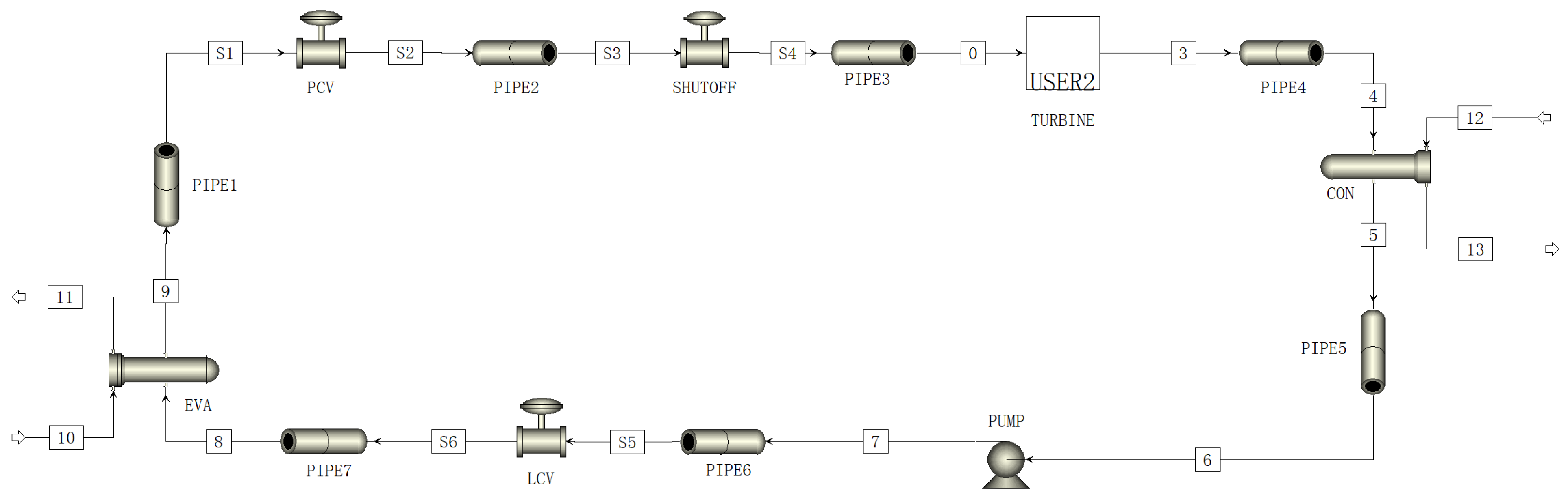
- There was no pipe fitting for adjustments in the pipe between the turbine outlet and the condenser inlet. The pipe structure and length were fixed. When the state parameters of the working fluid at one end of the pipeline and the flow parameters in the pipeline were determined, the state parameters of the working fluid at the other end are were determined. This is equivalent to indirectly controlling the turbine outlet pressure when the pressure control valve controls the condenser inlet pressure.
- The adjustment of the pressure control valve also affected the working fluid state parameters at the turbine inlet. This meant that the pressure control valve actively affected the state parameters of the three positions (turbine inlet and outlet and condenser inlet) at the same time.
- When the structure of a condenser was fixed, the heat exchange capacity of the condenser had an upper limit. If the condensing temperature was too low, meaning that the difference was small between the condensing temperature and the deep seawater temperature, the required deep seawater flow rate was too large when the heat exchange area was fixed. If the flow rate of the deep seawater was too large, the requirements for the deep seawater pump and deep seawater pipeline would be high, including structural size parameters, performance parameters and construction costs.
2.3. Simulation Condition Settings
3. Results
4. Conclusions
Author Contributions
Funding
Institutional Review Board Statement
Informed Consent Statement
Data Availability Statement
Acknowledgments
Conflicts of Interest
Appendix A
References
- Magesh, R. OTEC technology—A world of clean energy and water. In Proceedings of the World Congress on Engineering, London, UK, 30 June–2 July 2010. [Google Scholar]
- Chen, F. Research on Thermal Performance and Comprehensive Utilization of Ocean Thermoelectric Power Generation Device. Ph.D. Thesis, Harbin Engineering University, Harbin, China, 2016. [Google Scholar]
- Semmari, H.; Stitou, D.; Mauran, S. A novel Carnot-based cycle for ocean thermal energy conversion. Energy 2012, 43, 361–375. [Google Scholar] [CrossRef]
- Sun, F.; Zhou, W.; Nakagami, K. Energy-Economic Analysis and Configuration Design of the Kalina Solar-OTEC System. Int. J. Comput. Electr. Eng. 2013, 5, 187–191. [Google Scholar] [CrossRef]
- Yasunaga, T.; Noguchi, T.; Morisaki, T. Basic heat exchanger performance evaluation method on OTEC. J. Mar. Sci. Eng. 2018, 6, 32. [Google Scholar] [CrossRef] [Green Version]
- Fontaine, K.; Yasunaga, T.; Ikegami, Y. OTEC maximum net power output using Carnot cycle and application to simplify heat exchanger selection. Entropy 2019, 21, 1143. [Google Scholar] [CrossRef] [Green Version]
- Chen, Y.; Liu, Y.; Zhang, L.; Yang, X. Three-Dimensional Performance Analysis of a Radial-Inflow Turbine for Ocean Thermal Energy Conversion System. J. Mar. Sci. Eng. 2021, 9, 287. [Google Scholar] [CrossRef]
- Wu, Z.; Feng, H.; Chen, L. Optimal design of dual-pressure turbine in OTEC system based on constructal theory. Energy Convers. Manag. 2019, 201, 112179.1–112179.11. [Google Scholar] [CrossRef]
- Yoon, J.I.; Son, C.H.; Baek, S.M. Efficiency comparison of subcritical OTEC power cycle using various working fluids. Heat Mass Transf. 2014, 50, 985–996. [Google Scholar] [CrossRef]
- Seungtaek, L.; Hosaeng, L.; Junghyun, M. Simulation Data of Regional Economic Analysis of OTEC for Applicable Area. Processes 2020, 8, 1107. [Google Scholar] [CrossRef]
- Bernardoni, C.; Binotti, M.; Giostri, A. Techno-economic analysis of closed OTEC cycles for power generation. Renew. Energy 2019, 132, 1018–1033. [Google Scholar] [CrossRef]
- Giostri, A.; Romei, A.; Binotti, M. Off-design performance of closed OTEC cycles for power generation. Renew. Energy 2021, 170, 1353–1366. [Google Scholar] [CrossRef]
- Liu, W.M.; Chen, F.Y.; Wang, Y.Q. Progress of Closed-Cycle OTEC and Study of a New Cycle of OTEC. Adv. Mater. Res. 2012, 354–355, 275–278. [Google Scholar] [CrossRef]
- Kalina, A.I. Combined-Cycle System With Novel Bottoming Cycle. ASME J. Eng. Turbines Power 1984, 106, 737–742. [Google Scholar] [CrossRef]
- Ren, H. Effect of Low Ammonia Mass Fraction of the Base Solution on Theoretical Cycle Efficiency of Kalina Cycle System (kcs-34). J. Mech. Eng. 2012, 48, 152. [Google Scholar] [CrossRef]
- Ikegami, Y.; Yasunaga, T.; Harada, H. Performance Experiments on Ocean Thermal Energy Conversion System Using the Uehara Cycle. Bull. Soc. Sea Water Sci. Jpn. 2006, 60, 32–38. [Google Scholar]
- Uehara, H.; Ikegami, Y.; Nishida, T. Performance Analysis of OTEC System Using a Cycle with Absorption and Extraction Processes. Trans. Jpn. Soc. Mech. Eng. 1998, 64, 2750–2755. [Google Scholar] [CrossRef] [Green Version]
- Goto, S.; Motoshima, Y.; Sugi, T. Construction of simulation model for OTEC plant using Uehara cycle. Electr. Eng. Jpn. 2011, 176, 1–13. [Google Scholar] [CrossRef]
- Aydin, H.; Lee, H.S.; Kim, H.J.; Shin, S.K.; Park, K. Off-design performance analysis of a closed-cycle ocean thermal energy conversion system with solar thermal preheating and superheating. Renew. Energy 2014, 72, 154–163. [Google Scholar] [CrossRef]
- Park, S.; Chun, W.; Kim, N. Simulated production of electric power and desalination using Solar-OTEC hybrid system. Int. J. Energy Res. 2017, 41, 637–649. [Google Scholar] [CrossRef]
- Cui, Q. Research on Solar-assisted Ocean Thermal Energy Conversion System. IOP Conf. Ser. Earth Environ. Sci. 2021, 687, 012137. [Google Scholar] [CrossRef]
- Dugger, G.; Richards, D.; Paddison, F. Alternative ocean energy products and hybrid geothermal-OTEC/GEOTEC/plants. In Proceedings of the 2nd Terrestrial Energy Systems Conference, Colorado Springs, CO, USA, 1–3 December 1981; p. 2547. [Google Scholar]
- Idrus, N.; Musa, M.N.; Yahya, W.J. Geo-Ocean Thermal Energy Conversion (GeOTEC) power cycle/plant. Renew. Energy 2017, 111, 372–380. [Google Scholar] [CrossRef]
- Avery, W.H.; Wu, C. Renewable Energy from the Ocean: A Guide to OTEC; Oxford University Press: New York, NY, USA, 1994. [Google Scholar]
- Yue, J.; Yu, T.; Li, D. The latest progress and development suggestions of ocean thermoelectric power generation technology at home and abroad. J. Ocean. Technol. 2017, 36, 6. [Google Scholar]
- Makai Connects World’s Largest Ocean Thermal Plant to U.S. Grid. August 2015 [EB/OL]. Available online: http://www.makai.com/makai-news/2015_08_29_makai_connects_otec/ (accessed on 11 April 2022).
- Journoud, A.; Sinama, F.; Lucas, F. Experimental ocean thermal energy convemion (OTEC) project on the Reunion Island. In Proceedings of the 4th International Conference on Ocean Energy, Dublin, Ireland, 17–20 October 2012. [Google Scholar]
- Fontalvo, J. Using user models in Matlab within the Aspen Plus interface with an Excel link. Ing. Investig. 2014, 34, 39–43. [Google Scholar] [CrossRef]
- Ji, G. Turboexpander; Machinery Industry Press: Beijing, China, 1982. [Google Scholar]
- Keith Wait. Linking REFPROP with Other Applications (Matlab Applications). Available online: https://trc.nist.gov/refprop/LINKING/Linking.htm#MatLabApplications (accessed on 11 April 2022).
- Bulletin on the State of the Marine Environment in the South China Sea. 2012. Available online: http://scs.mnr.gov.cn/scsb/gbytj/201305/1f40063ea3404e9cbca7cd3d69e1b75e.shtml (accessed on 11 April 2022).
- Bulletin on the State of the Marine Environment in the South China Sea. 2013. Available online: http://scs.mnr.gov.cn/scsb/gbytj/201408/635886a23e3d4a64b6d90b1ac1cc0e6b.shtml (accessed on 11 April 2022).
- Bulletin on the State of the Marine Environment in the South China Sea. 2014. Available online: http://scs.mnr.gov.cn/scsb/gbytj/201505/381cf79ab8054fd6b4dcf67968b8202e.shtml (accessed on 11 April 2022).
- Bulletin on the State of the Marine Environment in the South China Sea. 2015. Available online: http://scs.mnr.gov.cn/scsb/gbytj/201607/edc0f44a77e44eb1bd5893db10fa463e.shtml (accessed on 11 April 2022).
- Bulletin on the State of the Marine Environment in the South China Sea. 2016. Available online: http://scs.mnr.gov.cn/scsb/gbytj/201706/e2cb33d595c74a22902c599c063d6b4c.shtml (accessed on 11 April 2022).


| Component | Type | Parameter | Value |
|---|---|---|---|
| Evaporator | Flooded | Working fluid location | Shell side |
| Heat exchange area | 301 m2 | ||
| Tube Type | Wieland 1575 fpm | ||
| Tube Material | Al-Brass | ||
| Condenser | Shell and Tube | Working fluid location | Shell side |
| Heat exchange area | 301 m2 | ||
| Tube type | Wieland 1575 fpm | ||
| Tube Material | Al-Brass | ||
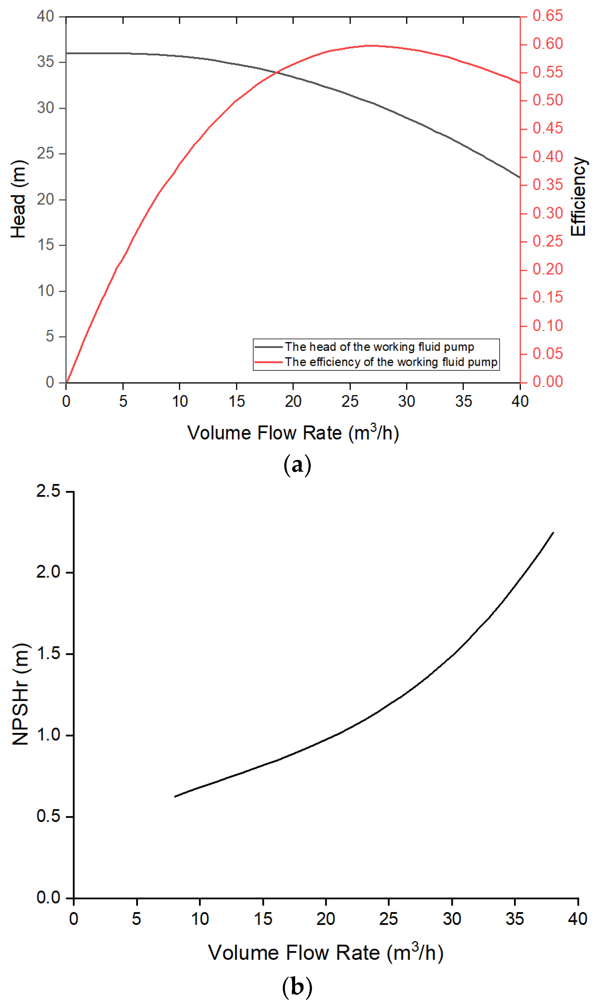
| Pump | Canned Motor | Rated flow rate | 24.2 m3/h |
| Rated head | 31.8 m | ||
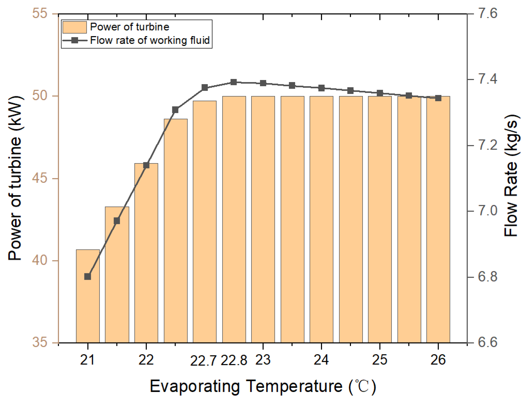
| Turbine | Centripetal | Rated speed | 12,500 rpm |
| Rated power | 50 kW |
| Tube Location | Nominal Diameter | Pipe Rise | Pipe Length | Miscellaneous L/D |
|---|---|---|---|---|
| At turbine inlet | DN150 | 2 m | 5.111 m | 160 |
| At condenser inlet | DN200 | −0.564 m | 6.075 m | 140 |
| At pump inlet | DN125 | −1.9 m | 2.47 m | 95 |
| At evaporator inlet | DN100 | 0 | 6.5 m | 135 |
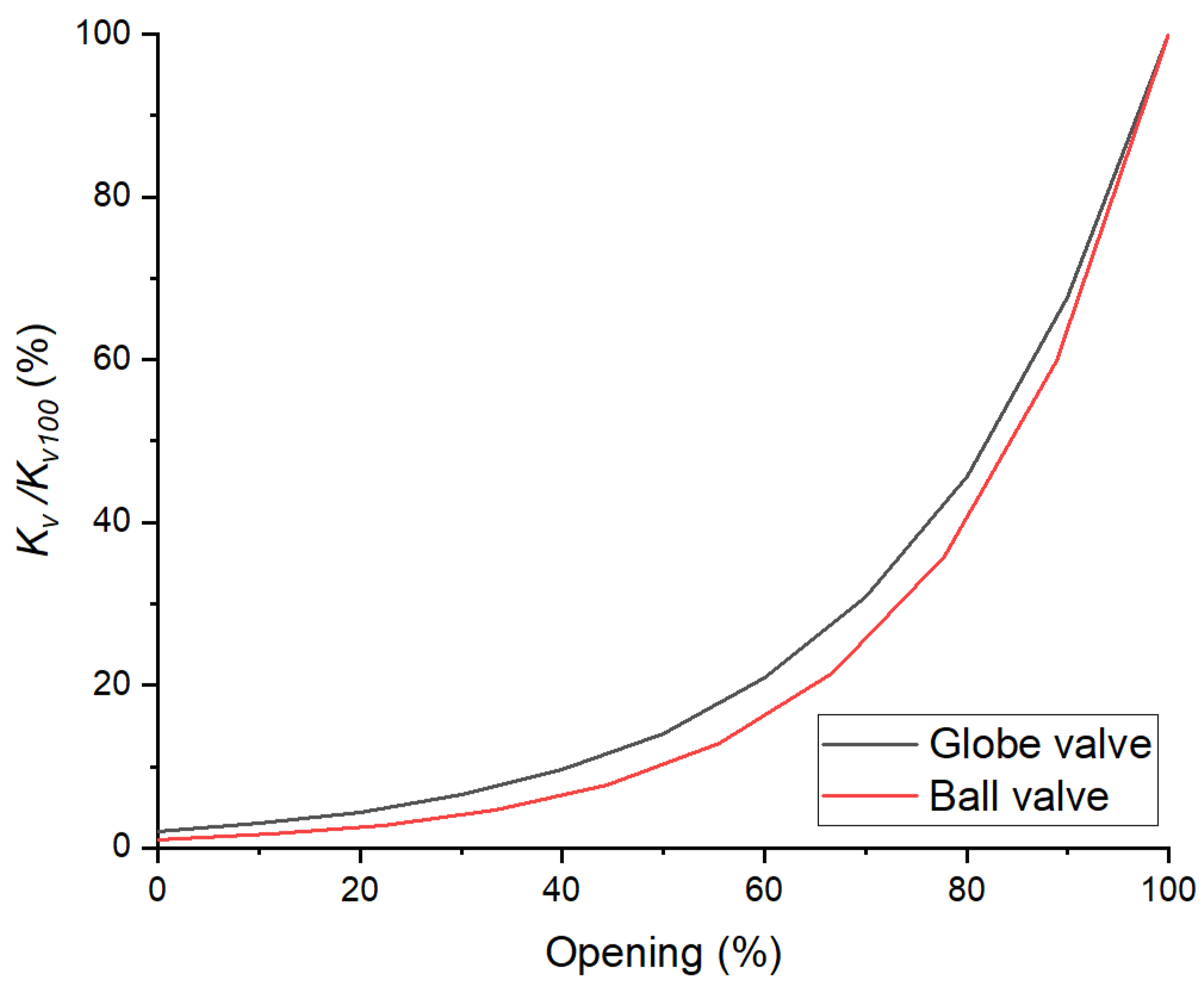
| Nominal Diameter | Type | Installation Location | |
|---|---|---|---|
| DN150 | Ball | 940 | At the turbine inlet |
| DN80 | Globe | 100 | At the evaporator inlet |
Publisher’s Note: MDPI stays neutral with regard to jurisdictional claims in published maps and institutional affiliations. |
© 2022 by the authors. Licensee MDPI, Basel, Switzerland. This article is an open access article distributed under the terms and conditions of the Creative Commons Attribution (CC BY) license (https://creativecommons.org/licenses/by/4.0/).
Share and Cite
Yang, X.; Liu, Y.; Chen, Y.; Zhang, L. Operation Control and Performance Analysis of an Ocean Thermal Energy Conversion System Based on the Organic Rankine Cycle. Energies 2022, 15, 3971. https://doi.org/10.3390/en15113971
Yang X, Liu Y, Chen Y, Zhang L. Operation Control and Performance Analysis of an Ocean Thermal Energy Conversion System Based on the Organic Rankine Cycle. Energies. 2022; 15(11):3971. https://doi.org/10.3390/en15113971
Chicago/Turabian StyleYang, Xiaowei, Yanjun Liu, Yun Chen, and Li Zhang. 2022. "Operation Control and Performance Analysis of an Ocean Thermal Energy Conversion System Based on the Organic Rankine Cycle" Energies 15, no. 11: 3971. https://doi.org/10.3390/en15113971