Abstract
Accurate short-term wind speed forecasting plays an important role in the development of wind energy. However, the inertia of airflow means that wind speed has the properties of time variance and inertia, which pose a challenge in the task of wind speed forecasting. We employ the variable support segment method to describe these two properties. We then propose a variable support segment-based short-term wind speed forecasting model to improve wind speed forecasting accuracy. The core idea is to adaptively determine the variable support segment of the future wind speed by a self-attention mechanism. Historical wind speed series are first decomposed into several components by variational mode decomposition (VMD). Then, the future values of each component are forecast using a modified Transformer model. Finally, the forecasting values of these components are summed to obtain the future wind speed forecasting values. Wind speed data collected from a wind farm were employed to validate the performance of the proposed model. The mean absolute error of the proposed model in spring, summer, autumn, and winter is 0.25, 0.33, 0.31, and 0.29, respectively. Experimental results show that the proposed model achieves significant accuracy and that the modified Transformer model has good performance.
1. Introduction
Wind energy has become the most promising clean energy due to its large reserves [1] and good foundation. The Global Wind Energy Council has indicated that the installed global wind power capacity provide be up to 20% of global electricity by 2030 [2]. The development and utilization of wind energy are critical to alleviating the pressure generated by traditional energy sources such as fossil fuels. The conversion and management of wind energy is closely related to wind speed. Accurate short-term wind speed forecasting, which estimates the wind speed 30 min to 6 h ahead [3], is essential for optimizing power grid scheduling, reducing system rotating reserve capacity, and guaranteeing stable grid operation [4,5]. However, the accuracy and reliability of wind speed forecasting are affected by the stochastic nature and nonlinear characteristics of wind speed. Various models for improving wind speed accuracy have been proposed [6,7,8,9], which can be divided into the categories of single models and combined models based on their structure. The most widely used single models include the backpropagation (BP) neural network [10], extreme learning machine (ELM), Kalman filtering, the autoregressive moving average (ARMA) [11], and support vector regression (SVR) [12] models.
A single model is unable to achieve satisfactory forecasting accuracy due to the intermittency of wind speed. Thus, combined models consisting of multiple single models are widely applied. Extensive studies have shown that combined models have better performance [13,14]. There are two sorts of combined models. The first weights the forecasting values of different models to obtain the final forecasting values. In [15], the weight coefficients of three different models were determined via modified support vector regression. In [16], the partial least squares algorithm was used to optimize the weight coefficients. Wang et al. [17] proposed a combined model in which the coefficients of four artificial neural networks’ forecasting results are determined using the multi-objective bat algorithm (MOBA).
However, the original wind speed series often appears as a broadband signal in the frequency domain, which is difficult to forecast directly. Therefore, a second sort of combined model has been presented to solve this issue. First, a historical wind speed series is broken into narrowband components using the signal decomposition method. Then, each narrowband component’s future values are forecast separately by the forecasting models. The final forecasting values are the sum of each component’s forecasting values. The most commonly used signal decomposition methods include wavelet transform (WT) [18], empirical mode decomposition (EMD) [19] and its variants, and variational mode decomposition (VMD) [20]. In [21], WT was employed to reduce wind speed fluctuation characteristics. Naik et al. [22] utilized EMD to preprocess wind speed data. In [23], VMD was used to overcome the intermittency of the wind and eliminate noise signals. WT requires the wavelet function and the decomposition layers to be selected artificially, which is non-adaptive. Although EMD and its variants are adaptive, they have limitations such as mode mixing and endpoint effect. VMD has good noise robustness, which is an adaptive signal decomposition method. Here, we employ VMD as the signal decomposition method.
Forecasting models are another key component of combined models; research [24,25] has shown that deep learning models have better performance in extracting and learning complex quantitative relationships hidden in wind speed data. Altan et al. [26] used the long short-term memory (LSTM) model for the forecasting of narrowband components, which showed good performance. In [27], the bidirectional LSTM model was utilized to forecast the sub-series. In [28], a combined model which incorporated VMD, differential evolution (DE), and echo state network (ESN) was proposed. In [29], the significant spatiotemporal characteristics in wind speed data were extracted by a graph deep learning model.
The Transformer model [30] is a deep learning model based on the self-attention mechanism which is good at capturing dependencies in long sequences and is not affected by distance. The Transformer model outperforms other deep learning models on process sequence data, hence, we employ it here as the forecasting model. However, the Transformer model cannot be employed for time series forecasting tasks directly due to its particular structure. Therefore, the structure of the Transformer model is modified in this paper. According to the above analysis, we first use VMD to obtain the narrowband components decomposed from historical wind speed series, then utilize the modified Transformer model to obtain each component’s forecasting values. The final forecasting values are the sum of each component’s forecasting values. The following are this paper’s major contributions:
- (1)
- We employ the variable support segment method to describe the time-varying and the inertia properties of wind speed;
- (2)
- We modify the Transformer model in order to approximate the variable support segment and complete the forecasting task of each narrowband component;
- (3)
- We propose a combined model based on the modified Transformer model and VMD. Two evaluation indicators and thirteen baseline models were used for a comparative experiment; the results indicate that our model has higher accuracy than comparative models and that the modified Transformer model outperforms other forecasting models.
The structure of this paper is as follows: Section 2 provides the mathematical description of wind speed forecasting; Section 3 briefly introduces VMD and the Transformer model; Section 4 presents the modified Transformer model and the proposed model; Section 5 analyzes the forecasting results of different models; and the final section contains our conclusions.
2. Mathematical Description of Wind Speed Forecasting
At present, most wind speed forecasting models assume that the future wind speed in the short term is only related to the historical wind speed:
where denotes the future wind speed series and denotes the historical wind speed series (i.e., the support segment of ); is the function that describes the mapping relationship between and . Thus, the wind speed forecasting task can be achieved by constructing a model to approximate the function f. Wind speed series often appear as broadband signals in the frequency domain, while narrowband signals are generally assumed to have a stable future trend and are easier to forecast. As a result, one feasible approach is to forecast the future values based on the narrowband components of historical wind speed series. The wind speed forecasting process based on signal decomposition can be formulated as
where , represents the narrowband component of the historical wind speed series, i.e.,the support segment of . Therefore, the function describes the quantitative relationships between and .
The inertia of airflow means that the wind speed shows time-varying and inertial properties, which influences the accuracy of wind speed forecasting. As Equation (2) fails to describe these two properties of wind speed effectively, there is room for improvement. Hence, the parameter , which is related to delay, can be introduced to the mathematical description of wind speed forecasting, and the parameter p, which denotes the length of the support segment, is set as a time variable. As a result, the mathematical description of wind speed forecasting can be formulated as
where is the variable support segment of . In Formula (3), the parameters and p vary with the historical wind speed series; thus, the inertia property of wind speed is described by the parameter , while the time-varying property of wind speed is described by the parameters and p jointly. When , Equation (3) corresponds to the one-step wind speed forecasting problem, which can be reformulated as
Unless otherwise specified, the remainder of this paper concentrates on the issue of one-step wind speed forecasting.
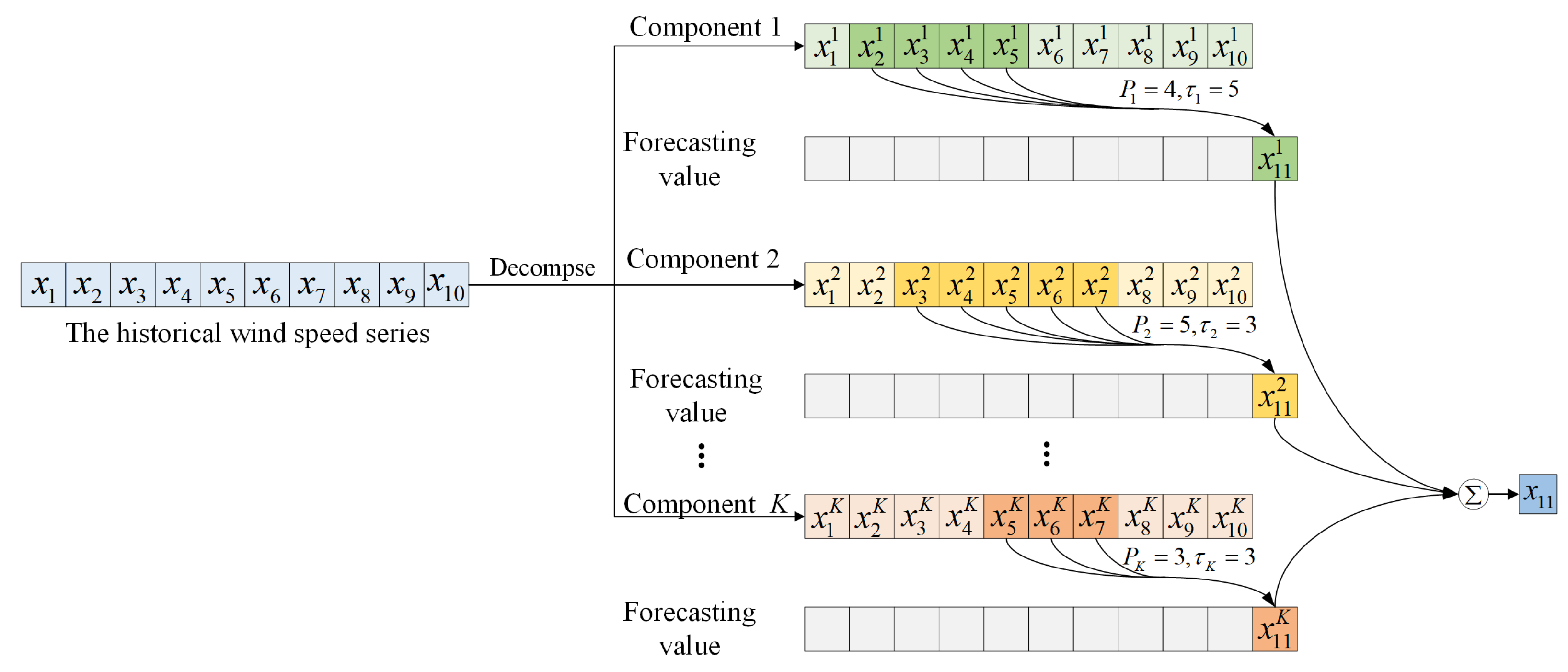
Figure 1 shows the schematic diagram of the variable support segment; , which contributes to the formation of , is the variable support segment of , that is, and . Similarly, the variable support segment of is ; and .
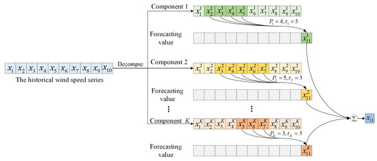
Figure 1.
Schematic diagram of the variable support segment.
According to Equation (4), we can forecast the future wind speed via the following steps.
- (1)
- Decompose the wind speed series into narrowband components based on the signal decomposition method;
- (2)
- Complete the forecasting task of each narrowband component by estimating the variable support segment corresponding to each narrowband component;
- (3)
- Superimpose the forecasting value of each narrowband component to obtain the future wind speed forecasting value.
Approximating the variable support segment accurately is the key to reducing the errors in wind speed forecasting. Existing forecasting models struggle with adaptively approximating the variable support segment. In our approach, the variable support segment is approximated using the self-attention mechanism, the specific process of which is introduced in Section 4.1.
3. VMD and Transformer
For the purposes of this paper, VMD was selected as the signal decomposition method and the Transformer model was selected as the forecasting model; this section briefly introduces them.
3.1. VMD
VMD decomposes an input signal into a number of intrinsic mode functions which are band-limited. It includes two main parts, variational problem construction and variational problem solving.
VMD uses an input signal, , equal to the sum of all the modes as its premise and seeks K mode functions, , to obtain the minimum sum of the estimated bandwidths of each mode. Thus, the constrained variational problem can be formulated as
where is the mode function, is the mode center frequency, K is the number of modes, is the Dirac disturibution, ∗ is convolution, and is the input signal.
By introducing the quadratic penalty term and the Lagrangian multiplier , the constrained variational problem of Equation (5) becomes an unconstrained variational problem:
In order to solve the unconstrained variational problem, VMD alternately updates , , and to find the “saddle point” of the extended Lagrangian expression. Here, the iterative formula of the Fourier transform of , and can be expressed as
where is an update factor.
3.2. The Transformer Model
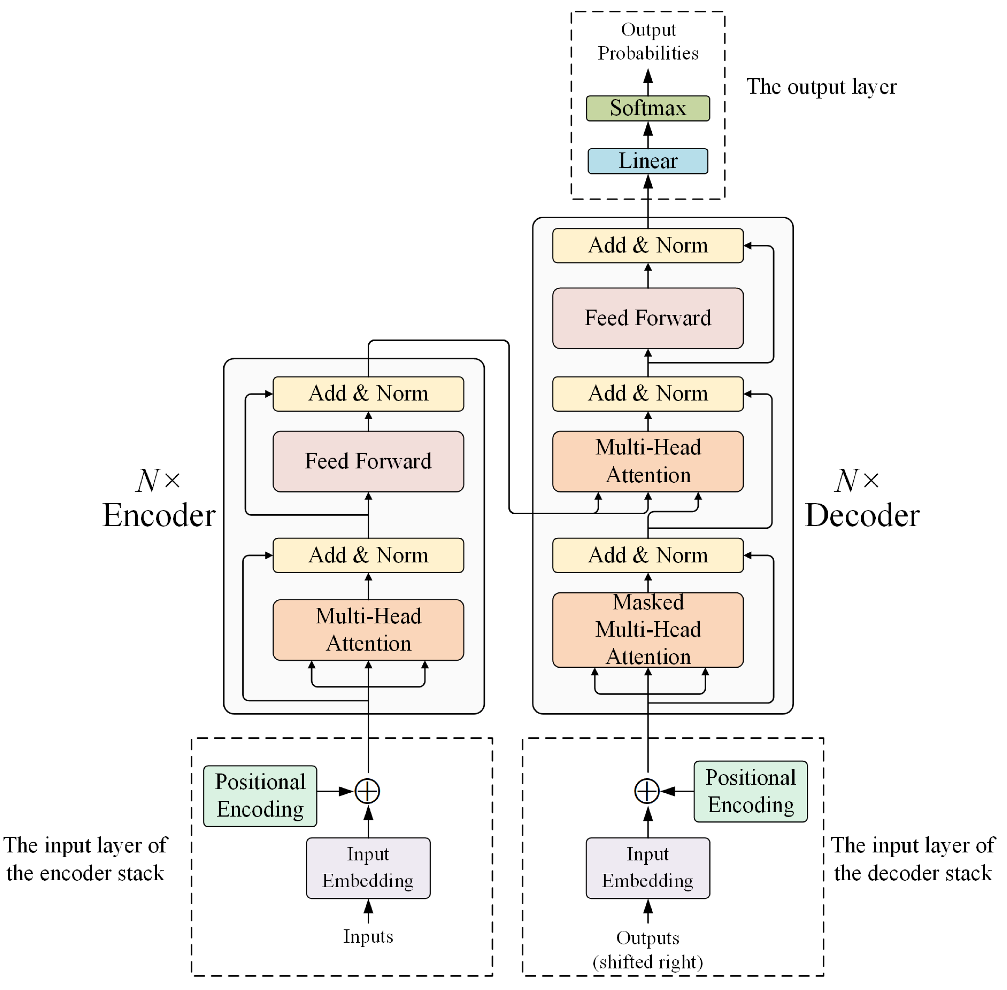
The Transformer [30] model is a model based on an “encoder–decoder” structure, shown in Figure 2. The model consists of an input layer, encoder stack, decoder stack, and output layer.
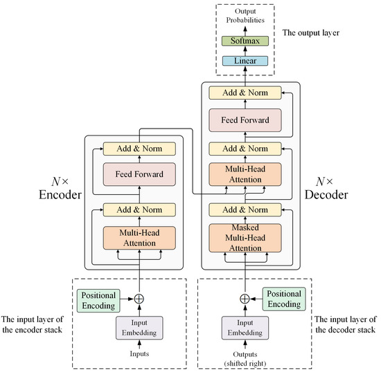
Figure 2.
The structure of the Transformer model.
The word embedding module and positional encoding module, which correspond to “Input Embedding” and “Positional Encoding” in Figure 2, respectively, make up the input layer. The word embedding module is utilized to convert input words into computable vectors, as words cannot be directly input into the model. The positional encoding module embeds positional information into the input sequence, as the Transformer model abandons the traditional recurrent neural network structure and is therefore unable to directly receive the position information of the input sequence. The encoder stack which is responsible for encoding the input information and generating intermediate vectors as the input of the decoder stack is composed of several encoders. Each encoder contains two modules, the multi-head attention mechanism module and the feed-forward neural network module, corresponding to “Multi-Head Attention” and “Feed Forward” in the Figure 2, respectively. Here, we use relu as the activation function in the feed-forward neural network module. Residual connections are used between each module and normalization is carried out, which is indicated by the “Add & Norm” part in the Figure 2.
The multi-head attention mechanism module calculates the attention based on a self-attention mechanism, which can deeply explore the internal relationship of input sequences, focus on important information, and filter out unimportant information. The self-attention mechanism first maps the input matrix into the query matrix , the key matrix , and the value matrix , then calculates the attention distribution by the scale dot production, and finally performs a weighted summation of the value matrix according to the attention distribution. Specifically, this is shown in Equations (10)–(13):
where , , and are the weight matrix corresponding to , , and , respectively, and is a scale factor.
The information learned by a single self-attention mechanism is relatively simple. In order to fully mine the correlation information between input sequences, the Transformer model further adopts the multi-head attention mechanism in order to learn information from different subspaces, then splices the outputs of different subspaces to obtain the final output, as shown in detail in Equations (14) and (15):
where , , and are the weight matrices corresponding to , and , in , is used to splice the output of each , and is the projection matrix, which is used to realize the projection of the stitching result.
The decoder stack, which is responsible for decoding the input information, is composed of several decoders. Compared to the encoder, the decoder includes an additional mask multi-head attention mechanism module to prevent information leakage. Residual connections between the modules of the decoder are used and normalized.
The output layer includes the Linear module and the Softmax module, which are used to convert the vector output by the decoder stack into a probability and then output the word corresponding to the highest probability.
4. The Wind Speed Forecasting Model
4.1. The Modified Transformer Model
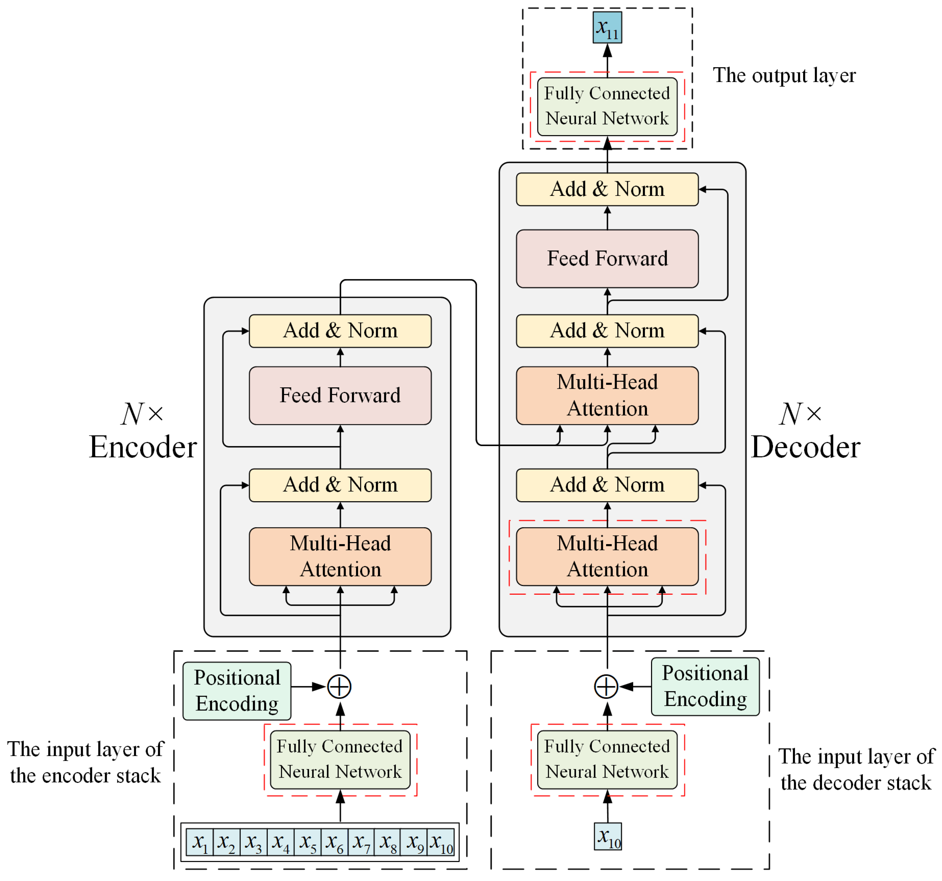
The structure of the original Transformer model is not suitable for time series forecasting tasks; therefore, we conducted several specific modifications:
- (1)
- The word-embedding module was replaced by a fully-connected neural network (FCNN) to allow the wind speed series to be input directly into the model;
- (2)
- In the decoder, the masked multi-head attention mechanism was replaced by a multi-head attention mechanism, as only a single data source is fed into the decoder stack and the information of the subsequent sequence is not subsequently involved;
- (3)
- The original output layer was removed and the output of the encoder stack directly mapped into the wind speed forecasting result from the FCNN.
For convenience, the modified Transformer model, shown in Figure 3, is called M-Transformer in this paper.

Figure 3.
The structure of the M-Transformer model.
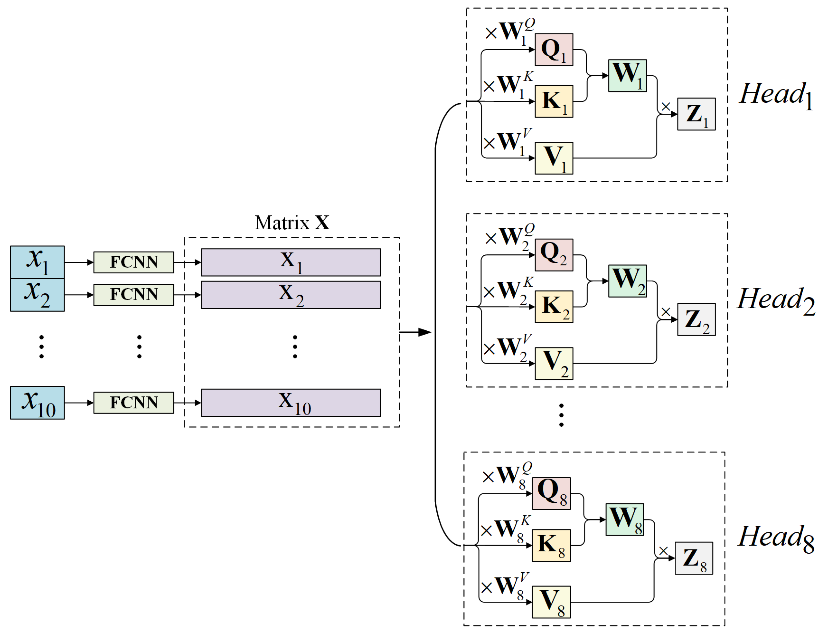
Drawing on the large number of previous experimental results, the number was set as 8 and the input length of the narrowband component as 10. Without loss of generality, the historical wind speed components were represented as . It should be noted that were fed into the FCNN. As shown in Figure 4, is mapped into a row vector by the FCNN with the length . The matrix is concatenated from ten row vectors generated from the narrowband modes of the historical wind speed, which is then fed into in order to separately calculate the attention distribution.

Figure 4.
The schematic diagram of the multi-head attention mechanism.
Using as an example, the matrix is multiplied by to generate , , . The attention distribution of (i.e., the weight matrix in Figure 4) is calculated based on Equation (16):
after which we multiply and value matrix to obtain the output of :
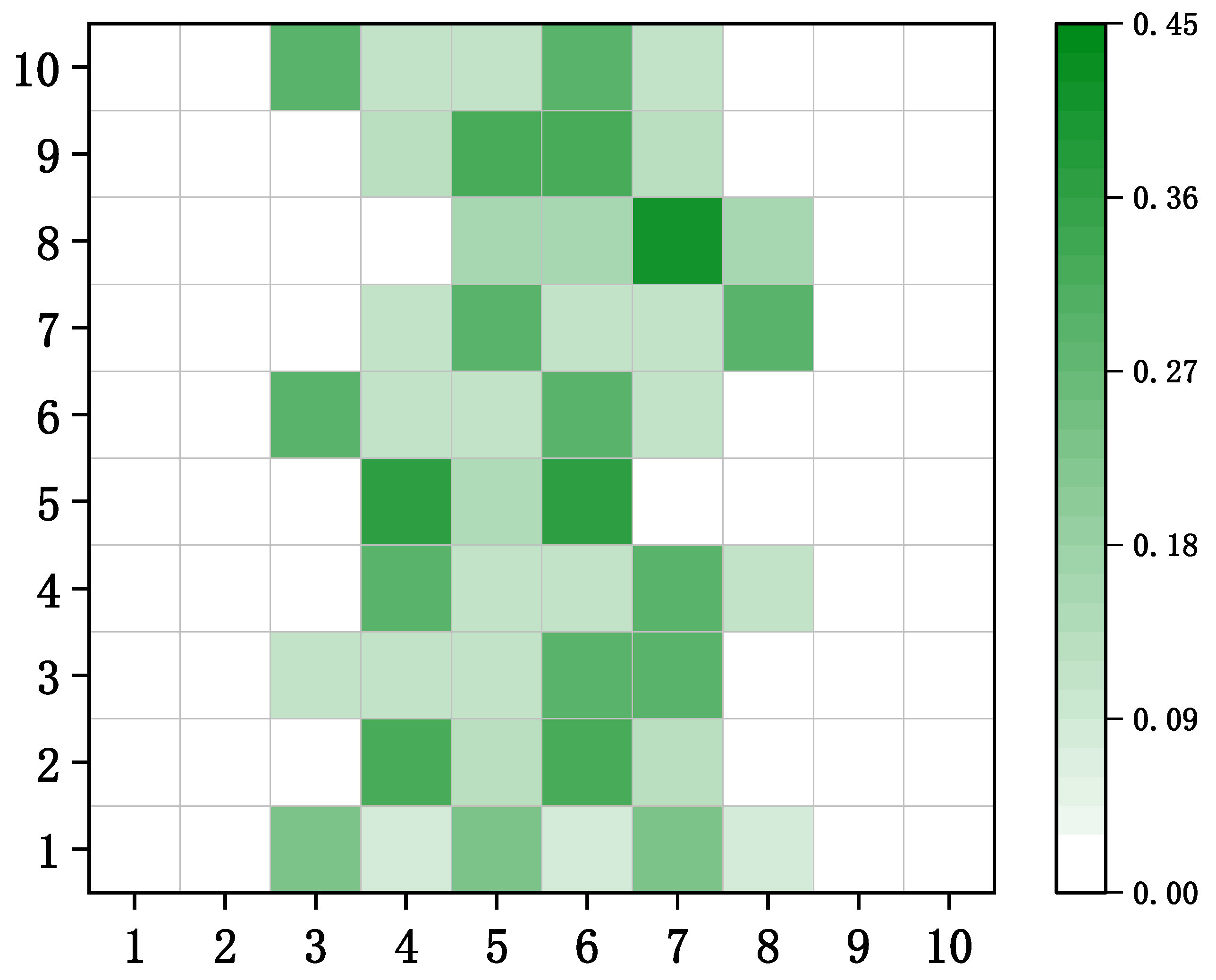
The ith row of can be considered as the weighted sum of all rows of the matrix , and the weight of each row is the numerical value of the corresponding element on the ith row of . The jth row of is determined by the unique historical wind speed component sample value ; thus, the weight matrix, , determines which sample values in the narrowband components of the historical wind speed series contribute to the output of . Thus, the weight matrices of all of the first encoder in the encoder stack together to determine the variable support segment of the narrowband modes of the historical wind speed series, which can be expressed as
where represents the jth column of the weight matrix of the hth and denotes the maximum element value of .
Figure 5 shows a pseudo-color figure of the weight matrix of the first of the first encoder in the encoder stack. It can be seen that the non-zero elements are concentrated in certain columns in , which is to say that in the component of the historical wind speed series, the only elements that contribute to the output of Head are .
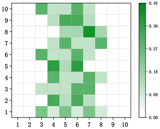
Figure 5.
The attention distribution of .
4.2. Proposed Model
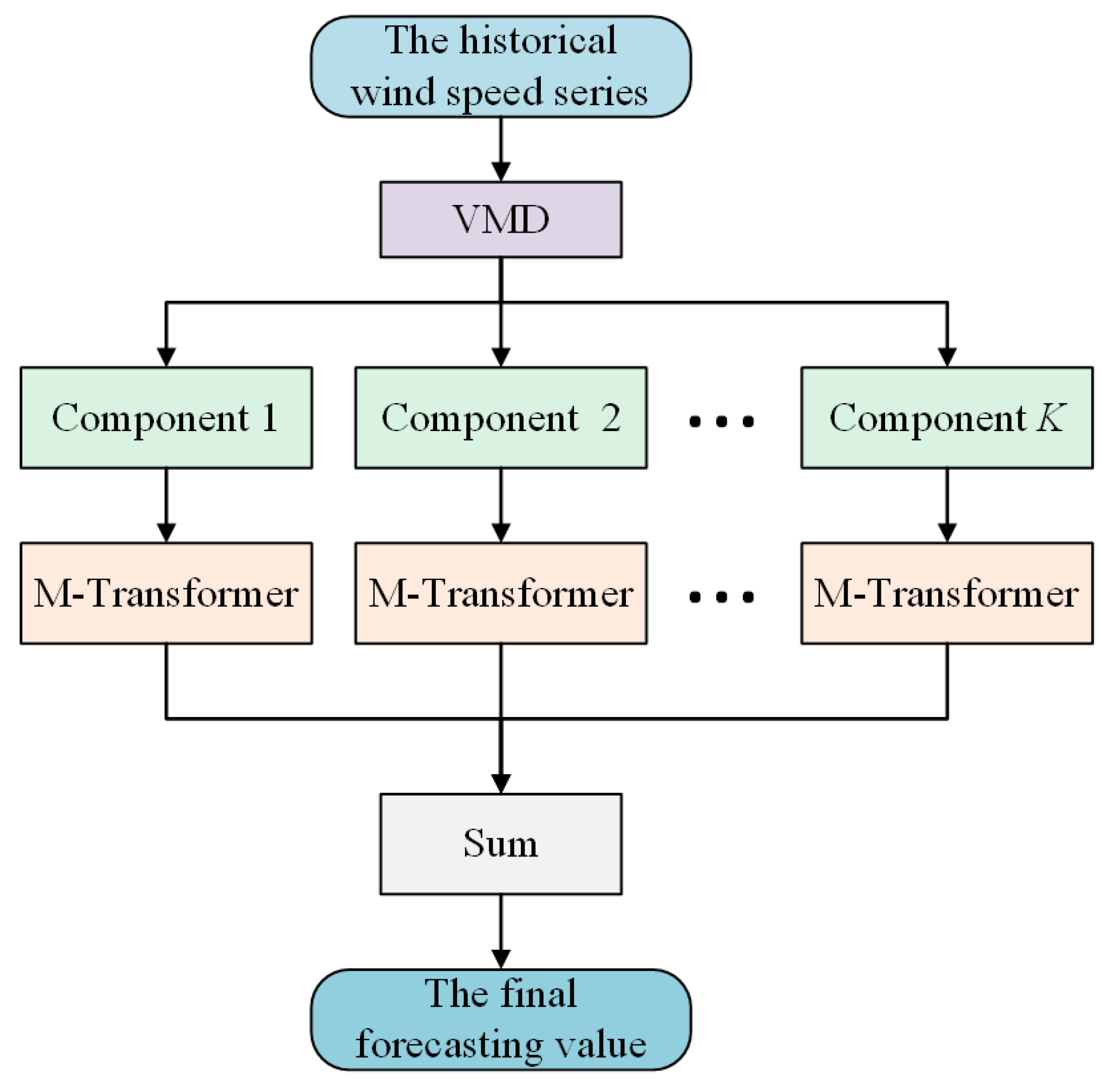
According to the wind speed forecasting task steps in Section 2, several narrowband components decomposed from the historical wind speed series are input into the M-Transformer model to separately obtain the forecasting value. The wind speed forecasting result is the sum of the forecasting value of each narrowband component. A flow chart for the proposed method is shown in Figure 6, abbreviated as VMD-TF for convenience.

Figure 6.
The flowchart of the proposed method.
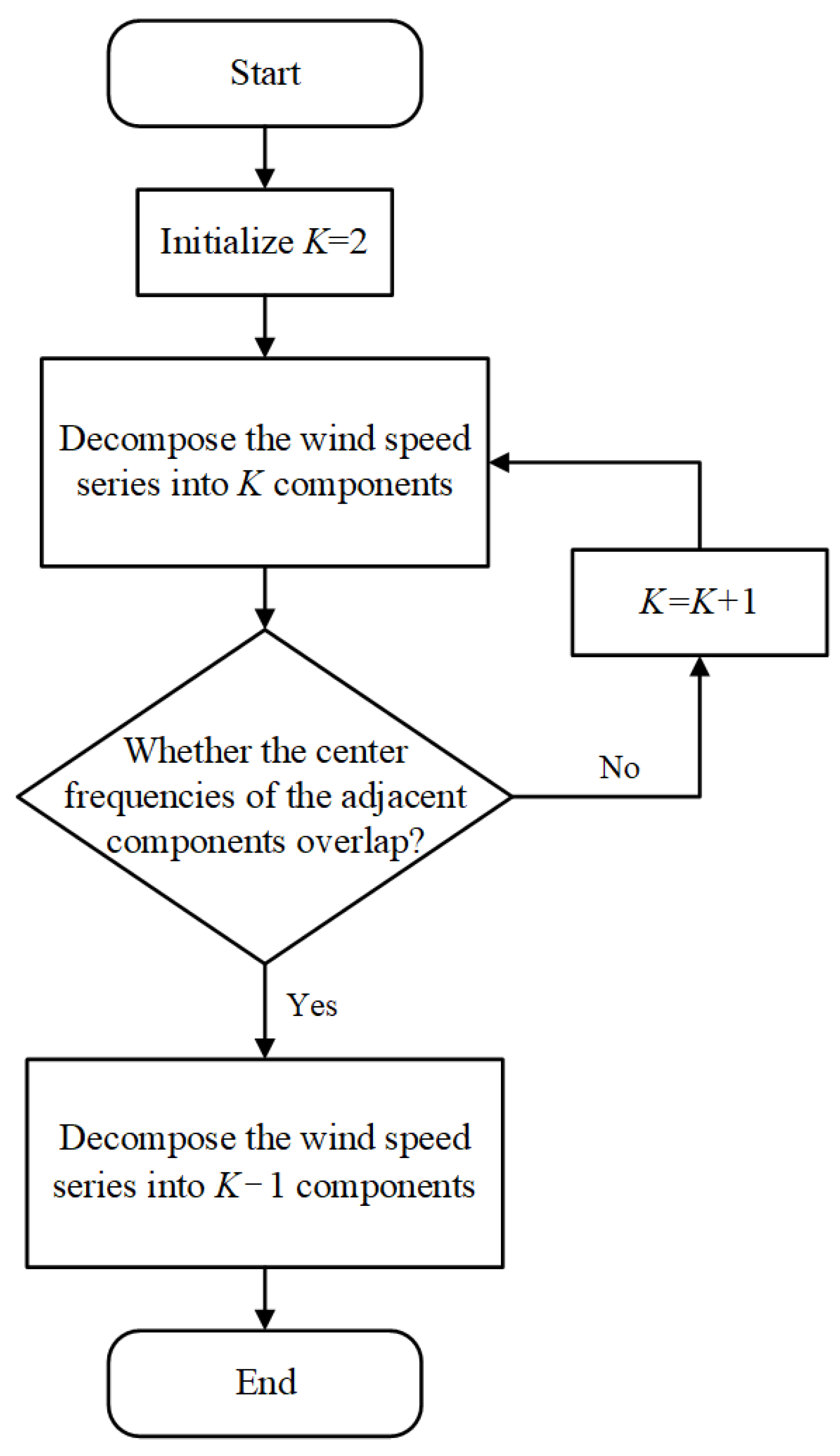
According to Figure 6, before decomposing the wind speed series based on the VMD, parameters K (i.e., the number of narrowband components) need to be determined. In our approach, these are determined by judging whether the center frequencies of the adjacent components overlap; the specific process is shown in Figure 7. The quadratic penalty factor influences the decomposition results. When the quadratic penalty factor is 2000, VMD has certain adaptability and can avoid mode mixing.

Figure 7.
Flowchart for determining K.
5. Experiment and Analysis
5.1. Wind Speed Data
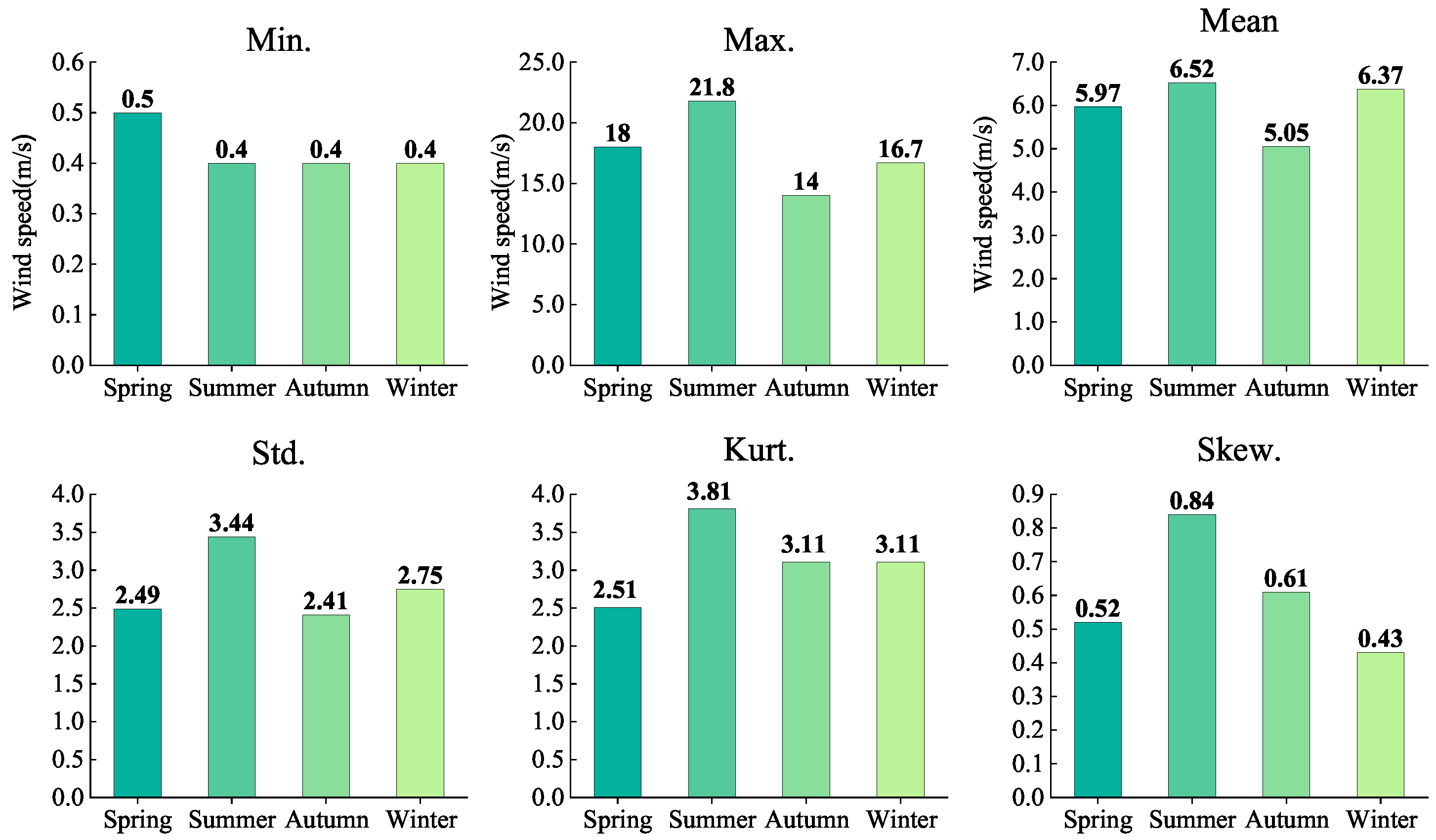
The data were obtained from a wind farm in Hebei. The sampling interval used in collecting the the data was 1 h. Hebei is located in a temperate monsoon climate, and the characteristics of the data consequently vary from season to season. Figure 8 shows the statistics related to the wind speed data in different seasons.

Figure 8.
Statistical data for wind speed in different seasons.
As can be seen in Figure 8, the maximum and average wind speed in summer is higher than in other seasons, indicating abundant wind energy resources. In addition, the wind speed in summer varies greatly and has strong randomness, with the highest standard deviation.
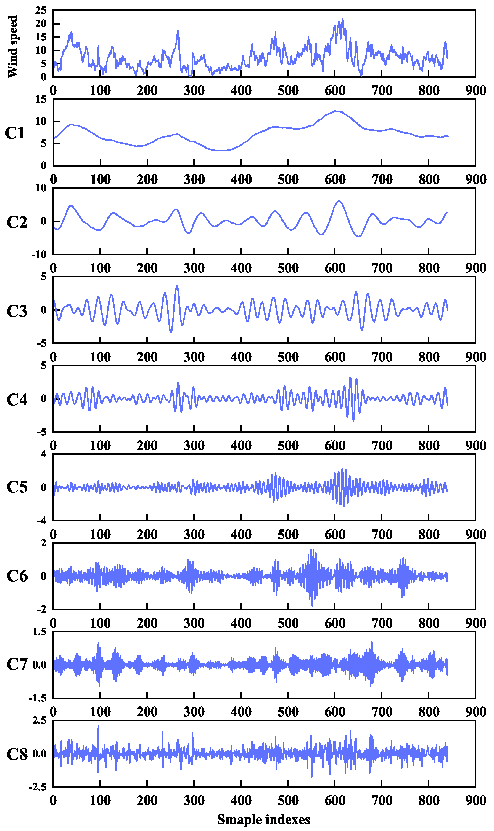
Figure 9 shows the decomposition result of the wind speed series from April 14th to May 18th, that is, in summer, in which – are narrowband components. It can be clearly seen that the trend of each component is more regular than the original wind speed series. is the residual component. Although it contains noise, it may contain part of the information of the original wind speed series as well. Therefore, permutation entropy was utilized to assess the signal’s randomness and determine whether the residual component could be considered a component of the original wind speed series.
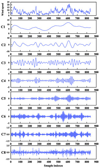
Figure 9.
Wind speed series decomposition results.
5.2. Accuracy Assessment
In this paper, the mean absolute error (MAE) and the root mean square error (RMSE) were selected as the evaluation indicators
where N is the length of the forecasting wind speed series, denotes the true value, and represents the forecasting value.
5.3. Results and Analysis
5.3.1. Forecasting Result
In each quarter, we randomly selected a week of wind speed data as the test set and used the four weeks of data before the test set as the training set; the specific division is shown in Table 1.

Table 1.
Division of the training and testing sets.
The parameters used for the M-Transformer were as follows: the encoder stack consisted of four encoders, the decoder stack contained four decoders, the dropout rate was equal to 0.1, the learning rate was set to 0.002, the batch size was set to 72 and 1 for the training and testing process, respectively, the optimizer was adma, and the loss function was the mean square error (MSE). Both the training and testing process were implemented in the Python 3.7 platform.
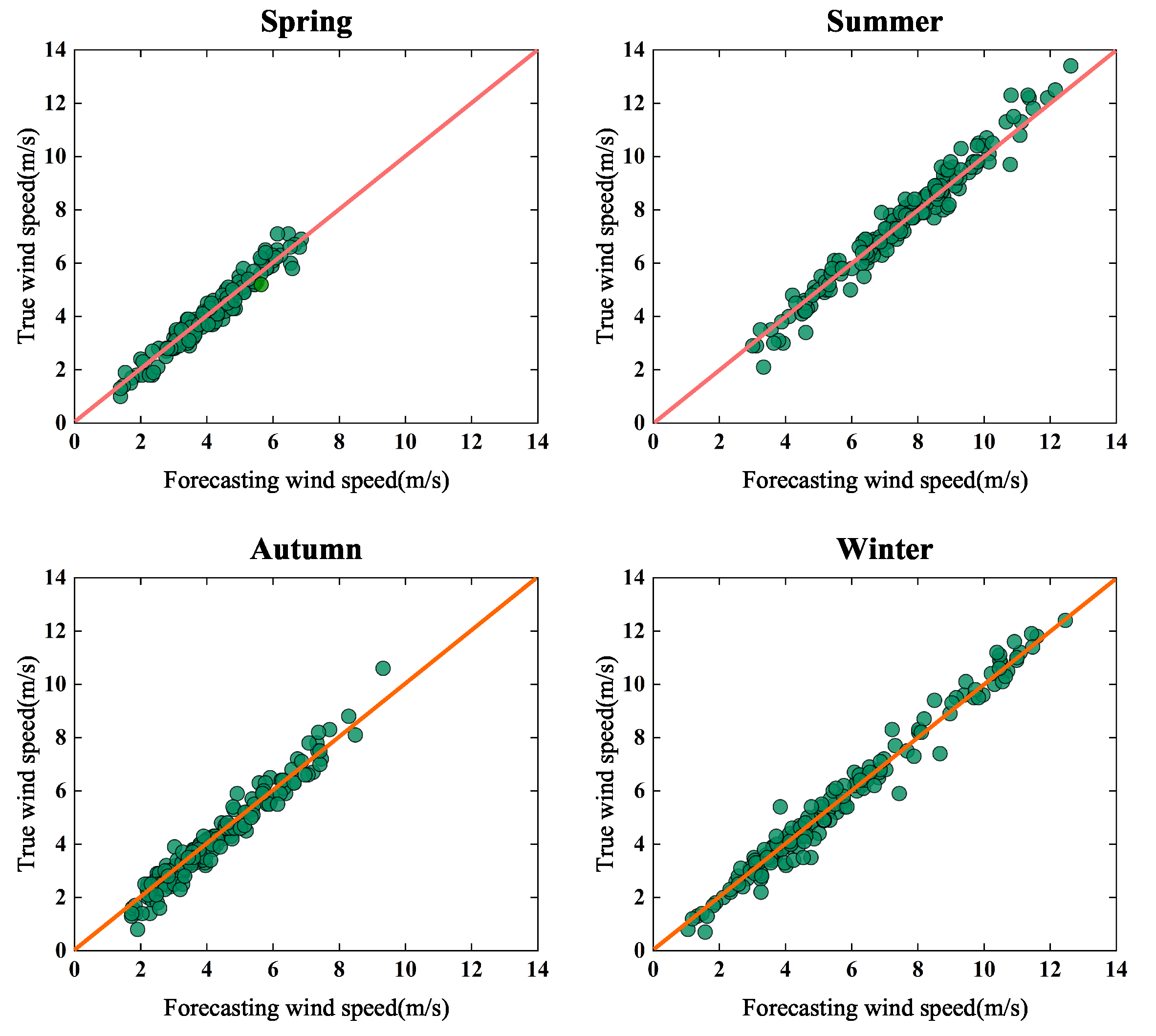
Figure 10 is a scatter diagram of the forecasting results for each season. The abscissa and ordinate are the forecasting and the true wind speed, respectively. The closer the data points are to the 45° line, the better the forecasting results. In Figure 10, the data points are closely distributed on the 45° line and on both sides, indicating that the proposed model achieves good performance.

Figure 10.
The forecasting results of the proposed model.
5.3.2. Comparative Experiments
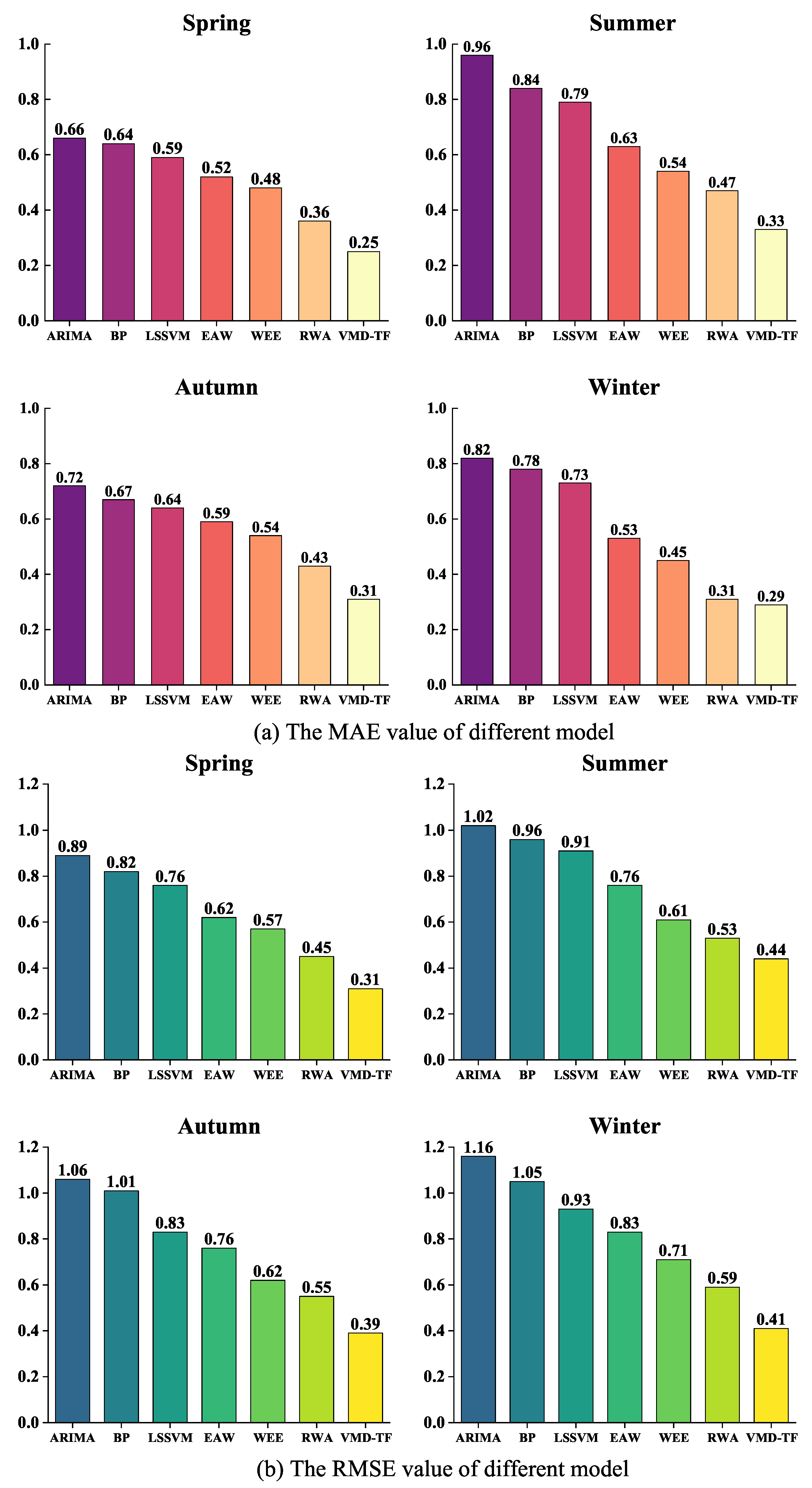
In this paper, three single models and three combined models were selected as comparison models to further verify the superiority of VMD-TF. The single models were ARIMA, BP, and LSSVM, and the combined models were EAW [31], WEE [32], and RWA [33]. The forecasting results of each model were evaluated by MAE and RMSE respectively, and the specifics are shown in Figure 11.
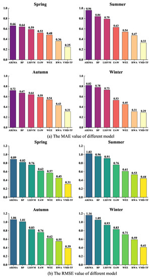
Figure 11.
The MAE and RMSE values of different models.
Equation (21) was utilized as the evaluation indicator to compare the improvement of VMD-TF to the other models:
Here, denotes the performance improvement index and and are the error of the VMD-TF and the comparison model, respectively. Table 2 shows the specific results.
Table 2.
The performance improvements achieved by the proposed model.
The results of the comparative experiment show the following.
- (1)
- VMD-TF outperforms the other six models. The performance of VMD-TF greatly increased compared with the single models. Using spring as an example, the MAE of VMD-TF fell by 62%, 61%, and 58% compared with ARIMA, BP, and LSSVM, respectively. The reason for this is that the potential of a single model to extract complicated characteristics is limited. However, VMD-TF shows better performance than the three combined models as well. Using autumn as an example, the RMSE of VMD-TF decreased by 49%, 37%, and 21% compared with EAW, WEE, and RWA, respectively, meaning that VMD-TF showed better feature extraction ability than the other combined models.
- (2)
- VMD-TF has the best performance in spring, followed by autumn and winter, and has relatively poor forecasting results in the summer. The properties of the wind speed data in each season have a high relation with the aforementioned results. According to Figure 8, the standard deviation of the summer data are all higher than those in other seasons, indicating that the wind speed in summer fluctuates greatly and is difficult to forecast.
- (3)
- The preceding results illustrate that VMD-TF achieves significant performance. The self-attention mechanism can adjust the attention distribution in a timely fashion according to the input data and realize adaptive estimation of the variable support segment, which is essential for improving wind speed forecasting accuracy.
5.3.3. Effectiveness of VMD
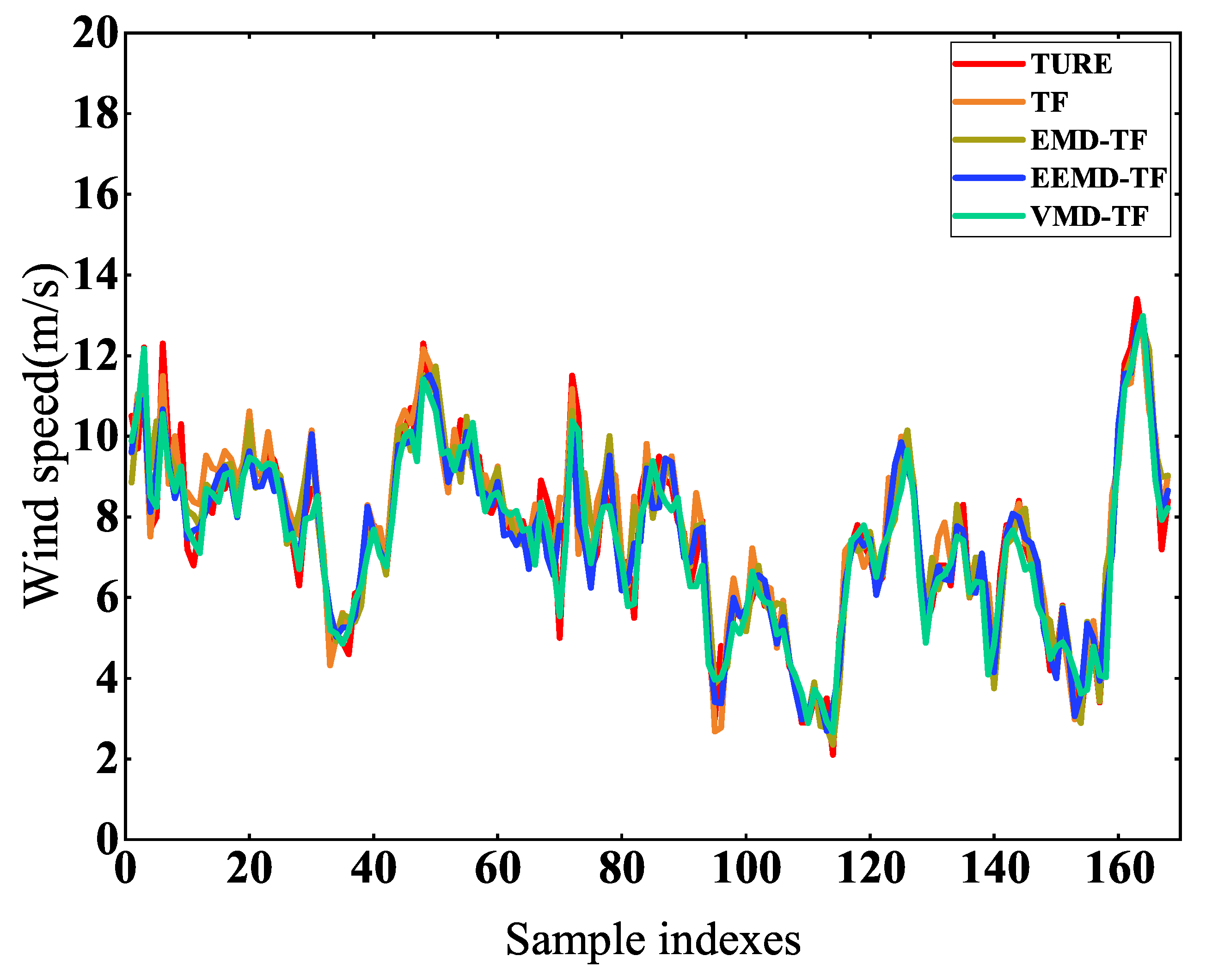
We employed EMD and EEMD as comparison methods to demonstrate that VMD could effectively reduce the influence of wind speed non-stationarity. The model combining M-Transformer with EMD is referred to as EMD-TF, while the model combining M-Transformer with EEMD is referred to as EEMD-TF. We used M-Transformer to forecast the wind speed directly without decomposition, in which case it is referred to as TF. In analyzing the capability of these models, the summer testing set was used. Figure 12 exhibits the comparisons between the forecasting values and the true values, while Table 3 shows the forecasting errors for each model.

Figure 12.
Comparison of the forecast and true wind speed for summer testing data.
Table 3.
The forecasting errors of each model with the summer testing data.
According to Figure 12, even when the wind speed changes greatly VMD-TF is able to track and forecast well, while TF, EMD-TF, and EEMD-TF cannot respond as well to such mutations. According to Table 3, the forecasting result with VMD-TF is the best, while TF is the worst. Thus, we are able to conclude that signal decomposition methods can greatly enhance wind speed forecasting accuracy, and that of the methods investigated here, VMD shows the best performance.
5.3.4. Effectiveness of M-Transformer
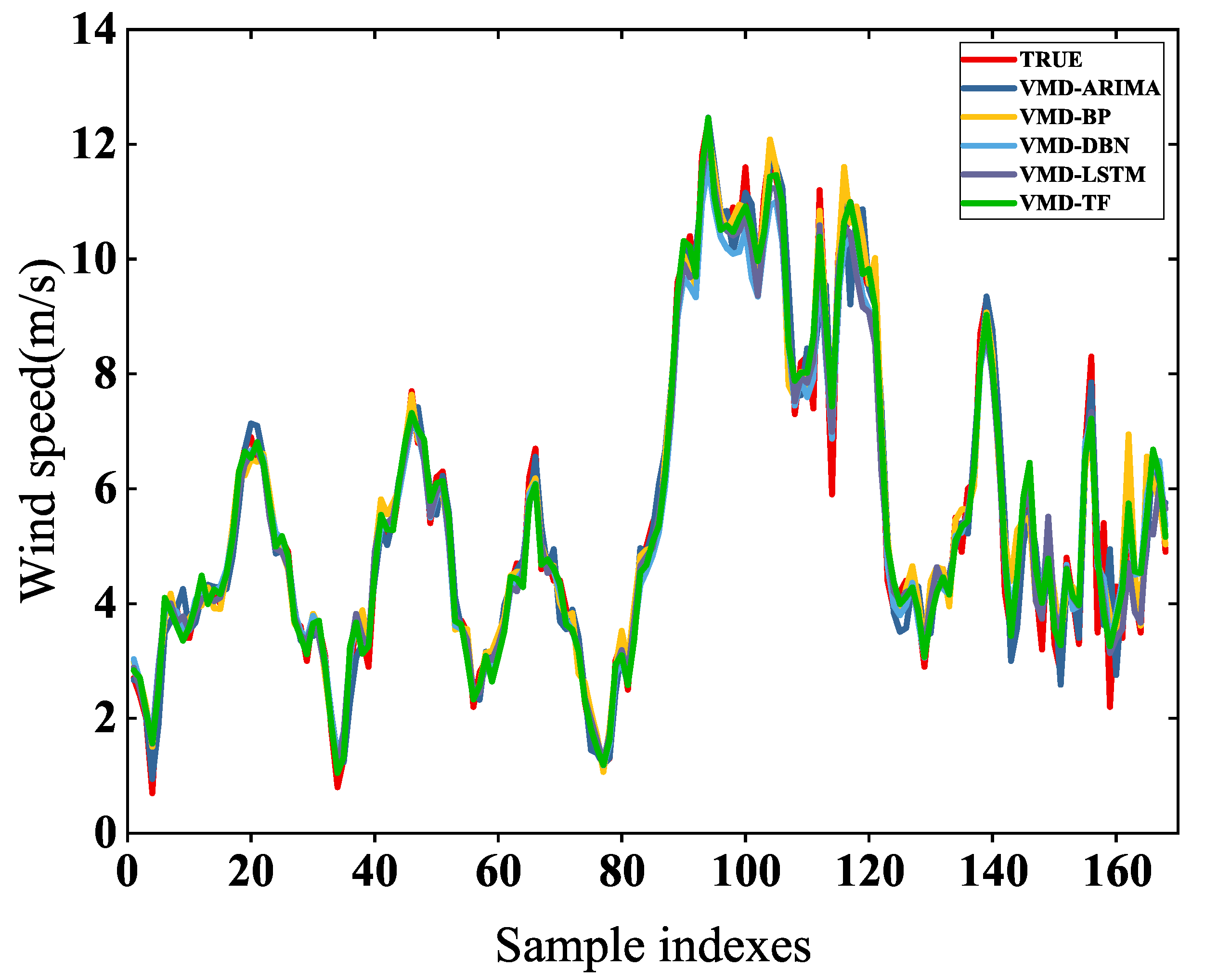
In order to illustrate that the M-Transformer model has good forecasting ability, we selected ARIMA, BP, the deep belief network (DBN), and LSTM as comparisons. These models, each composed of VMD and a single model, are referred to as VMD-ARIMA, VMD-BP, VMD-DBN, and VMD-LSTM, respectively. To assess the performance of these combined models, the winter testing set was used. Figure 13 compares the forecasting values and true values, while Table 4 shows the forecasting errors for each combined model.

Figure 13.
Comparison of forecast and real wind speed with winter testing data.
Table 4.
The forecasting errors of each combined model with the winter testing data.
In Figure 13, all forecasting wind speed curves appear to be relatively close to the true wind speed curve. According to Table 4, however, the MAE and RMSE of VMD-TF are the smallest. Taking MAE as an example, the accuracy of VMD-TF decreased by 33%, 17%, 15%, and 9%, respectively, compared with the other four models, which shows that M-Transformer has superior performance.
6. Conclusions
In this paper, we have proposed a variable support segment-based short-term wind speed forecasting model. Several conclusions can be drawn based on our experiments and analysis.
- (1)
- VMD has a better decomposition effect than EMD and EEMD, and can effectively reduce the effects of wind speed non-stationarity.
- (2)
- The M-Transformer model fully utilizes the characteristics of the self-attention mechanism, which can deeply mine potential information from wind speed series, estimate the variable support segment, and outperform other models in time series forecasting.
- (3)
- VMD-TF combines the advantages of VMD and the self-attention mechanism, achieving significantly improved performance.
Although VMD-TF shows significant performance achievements, it neglects the impact of meteorological factors, which limits its ability to deal with sudden changes in wind speed. In future work, we intend to develop a model that is able to take into account both historical wind speed data and prevailing meteorological factors that influence wind speed.
Author Contributions
Conceptualization, K.Z.; methodology, K.Z. and X.L.; software, K.Z.; validation, X.L.; formal analysis, J.S.; investigation, X.L.; resources, J.S.; data curation, K.Z.; writing—original draft preparation, K.Z.; writing—review and editing, X.L. and J.S.; visualization, X.L.; supervision, J.S.; project administration, J.S. All authors have read and agreed to the published version of the manuscript.
Funding
This research received no external funding.
Institutional Review Board Statement
Not applicable.
Informed Consent Statement
Not applicable.
Data Availability Statement
Not applicable.
Conflicts of Interest
The authors declare no conflict of interest.
References
- Shang, Z.; He, Z.; Chen, Y.; Xu, M. Short-term wind speed forecasting system based on multivariate time series and multi-objective optimization. Energy 2022, 238, 122024. [Google Scholar] [CrossRef]
- Wang, H.Z.; Wang, G.B.; Li, G.Q.; Peng, J.C.; Liu, Y.T. Deep belief network based deterministic and probabilistic wind speed forecasting approach. Appl. Energy 2016, 182, 80–93. [Google Scholar] [CrossRef]
- Dhiman, H.S.; Deb, D. A review of wind speed and wind power forecasting techniques. arXiv 2020, arXiv:2009.02279. [Google Scholar]
- Huang, X.; Wang, J.; Huang, B. Two novel hybrid linear and nonlinear models for wind speed forecasting. Energy Convers. Manag. 2021, 238, 114162. [Google Scholar] [CrossRef]
- Liu, F.; Li, R.; Li, Y.; Cao, Y.; Panasetsky, D.; Sidorov, D. Short-term wind power forecasting based on TS fuzzy model. In Proceedings of the 2016 IEEE PES Asia-Pacific Power and Energy Engineering Conference (APPEEC), Xi’an, China, 5–28 October 2016; pp. 414–418. [Google Scholar]
- Moreno, S.R.; Mariani, V.C.; Dos Santos Coelho, L. Hybrid multi-stage decomposition with parametric model applied to wind speed forecasting in Brazilian Northeast. Renew. Energy 2021, 164, 1508–1526. [Google Scholar] [CrossRef]
- Fu, W.; Zhang, K.; Wang, K.; Wen, B.; Fang, P.; Zou, F. A hybrid approach for multi-step wind speed forecasting based on two-layer decomposition, improved hybrid DE-HHO optimization and KELM. Renew. Energy 2021, 164, 211–229. [Google Scholar] [CrossRef]
- Sun, S.; Fu, J.; Li, A.; Zhang, P. A new compound wind speed forecasting structure combining multi-kernel LSSVM with two-stage decomposition technique. Soft Comput. 2021, 25, 1479–1500. [Google Scholar] [CrossRef]
- Luo, L.; Li, H.; Wang, J.; Hu, J. Design of a combined wind speed forecasting system based on decomposition-ensemble and multi-objective optimization approach. Appl. Math. Model. 2021, 89, 49–72. [Google Scholar] [CrossRef]
- Ren, C.; An, N.; Wang, J.; Li, L.; Hu, B.; Shang, D. Optimal parameters selection for BP neural network based on particle swarm optimization: A case study of wind speed forecasting. Knowl. Based Syst. 2014, 56, 226–239. [Google Scholar] [CrossRef]
- Erdem, E.; Shi, J. ARMA based approaches for forecasting the tuple of wind speed and direction. Appl. Energy 2011, 88, 1405–1514. [Google Scholar] [CrossRef]
- Santamaría-Bonfil, G.; Reyes-Ballesteros, A.; Gershenson, C. Wind speed forecasting for wind farms: A method based on support vector regression. Renew. Energy 2016, 85, 790–809. [Google Scholar] [CrossRef]
- Nie, Y.; Liang, N.; Wang, J. Ultra-short-term wind-speed bi-forecasting system via artificial intelligence and a double-forecasting scheme. Appl. Energy 2021, 301, 117452. [Google Scholar] [CrossRef]
- Zhou, Q.; Wang, C.; Zhang, G. A combined forecasting system based on modified multi-objective optimization and sub-model selection strategy for short-term wind speed. Appl. Soft Comput. 2020, 94, 106463. [Google Scholar] [CrossRef]
- Li, H.; Wang, J.; Lu, H.; Guo, Z. Research and application of a combined model based on variable weight for short term wind speed forecasting. Renew. Energy 2018, 116, 669–684. [Google Scholar] [CrossRef]
- Jiang, P.; Li, C. Research and application of an innovative combined model based on a modified optimization algorithm for wind speed forecasting. Measurement 2018, 124, 395–412. [Google Scholar] [CrossRef]
- Wang, J.; Heng, J.; Xiao, L.; Wang, C. Research and application of a combined model based on multi-objective optimization for multi-step ahead wind speed forecasting. Energy 2017, 125, 591–613. [Google Scholar] [CrossRef]
- Mallat, S.G. A theory for multiresolution signal decomposition: The wavelet representation. IEEE Trans. Pattern Anal. Mach. Intell. 1989, 11, 674–693. [Google Scholar] [CrossRef] [Green Version]
- Huang, N.E.; Shen, Z.; Long, S.R.; Wu, M.C.; Shih, H.H.; Zheng, Q.; Yen, N.C.; Tung, C.C.; Liu, H.H. The empirical mode decomposition and the Hilbert spectrum for nonlinear and non-stationary time series analysis. Proc. R. Soc. Lond. Ser. A Math. Phys. Eng. Sci. 1998, 454, 903–995. [Google Scholar] [CrossRef]
- Dragomiretskiy, K.; Zosso, D. Variational mode decomposition. IEEE Trans. Signal Process. 2013, 62, 531–544. [Google Scholar] [CrossRef]
- Memarzadeh, G.; Keynia, F. A new short-term wind speed forecasting method based on fine-tuned LSTM neural network and optimal input sets. Energy Convers. Manag. 2020, 213, 112824. [Google Scholar] [CrossRef]
- Naik, J.; Satapathy, P.; Dash, P.K. Short-term wind speed and wind power prediction using hybrid empirical mode decomposition and kernel ridge regression. Appl. Soft Comput. 2018, 70, 1167–1188. [Google Scholar] [CrossRef]
- Moreno, S.R.; da Silva, R.G.; Mariani, V.C.; dos Santos Coelho, L. Multi-step wind speed forecasting based on hybrid multi-stage decomposition model and long short-term memory neural network. Energy Convers. Manag. 2020, 213, 112869. [Google Scholar] [CrossRef]
- Jiang, P.; Liu, Z.; Niu, X.; Zhang, L. A combined forecasting system based on statistical method, artificial neural networks, and deep learning methods for short-term wind speed forecasting. Energy 2021, 217, 119361. [Google Scholar] [CrossRef]
- Liu, H.; Mi, X.; Li, Y. Wind speed forecasting method based on deep learning strategy using empirical wavelet transform, long short term memory neural network and Elman neural network. Energy Convers. Manag. 2018, 156, 498–514. [Google Scholar] [CrossRef]
- Altan, A.; Karasu, S.; Zio, E. A new hybrid model for wind speed forecasting combining long short-term memory neural network, decomposition methods and grey wolf optimizer. Appl. Soft Comput. 2021, 100, 106996. [Google Scholar] [CrossRef]
- Neshat, M.; Nezhad, M.M.; Abbasnejad, E.; Mirjalili, S.; Tjernberg, L.B.; Garcia, D.A.; Alexander, B.; Wagner, M. A deep learning-based evolutionary model for short-term wind speed forecasting: A case study of the Lillgrund offshore wind farm. Energy Convers. Manag. 2021, 236, 114002. [Google Scholar] [CrossRef]
- Hu, H.; Wang, L.; Tao, R. Wind speed forecasting based on variational mode decomposition and improved echo state network. Renew. Energy 2021, 164, 729–751. [Google Scholar] [CrossRef]
- Khodayar, M.; Wang, J. Spatio-temporal graph deep neural network for short-term wind speed forecasting. IEEE Trans. Sustain. Energy 2018, 10, 670–681. [Google Scholar] [CrossRef]
- Vaswani, A.; Shazeer, N.; Parmar, N.; Uszkoreit, J.; Jones, L.; Gomez, A.N.; Kaiser, Ł.; Polosukhin, I. Attention is all you need. Adv. Neural Inf. Process. Syst. 2017, 30, 5998–6008. [Google Scholar]
- Santhosh, M.; Venkaiah, C.; Kumar, D.M.V. Ensemble empirical mode decomposition based adaptive wavelet neural network method for wind speed prediction. Energy Convers. Manag. 2018, 168, 482–493. [Google Scholar] [CrossRef]
- Liu, H.; Mi, X.; Li, Y. An experimental investigation of three new hybrid wind speed forecasting models using multi-decomposing strategy and ELM algorithm. Renew. Energy 2018, 123, 694–705. [Google Scholar] [CrossRef]
- Singh, S.N.; Mohapatra, A. Repeated wavelet transform based ARIMA model for very short-term wind speed forecasting. Renew. Energy 2019, 136, 758–768. [Google Scholar]
Publisher’s Note: MDPI stays neutral with regard to jurisdictional claims in published maps and institutional affiliations. |
© 2022 by the authors. Licensee MDPI, Basel, Switzerland. This article is an open access article distributed under the terms and conditions of the Creative Commons Attribution (CC BY) license (https://creativecommons.org/licenses/by/4.0/).