Abstract
The impact of average wages on electricity consumption among urban residents in China has generated many fascinating debates for scholarly research, but only a few studies have considered the spatial spillover effect of average wages on residential electricity consumption. With the use of city-level panel data from 278 Chinese cities spanning 2005 to 2016, this preliminary study explores the impacts of the average wage on residential electricity consumption. Specifically, based on the spatial Durbin model with fixed effects, three different spatial weight matrices (the economic distance, the inverse distance, and the four nearest neighbours) are utilised to check the robustness of the results under different standards. The results show that the residential electricity consumption of each city increased during the observation period, presenting obvious spatial correlations. Secondly, the average wage of residents had a positive spatial spillover effect, which promoted the residential electricity consumption of both local and surrounding cities. Thirdly, the population density, electricity intensity, educational level of urban residents, and per capita household liquefied petroleum gas consumption in urban areas are key factors influencing residential electricity consumption. Therefore, improving the educational level of urban residents and reducing the electricity intensity can help reduce electricity consumption by residents in China. This paper also presents policy recommendations.
1. Introduction
Energy plays a vital role in promoting social progress and economic development. Electricity is a clean secondary energy source generated from primary natural energy sources such as raw coal, crude oil, and natural gas [1], and plays a huge role in people’s lives, industrial development, and economic growth. The domestic sector comprises one of the major areas of electricity consumption. As urbanisation and industrialisation continue to advance, China’s residential electricity consumption has seen steady growth. In particular, from 2005 to 2016, China’s total residential electricity consumption increased from 288.5 billion kWh to 842.06 billion kWh, with an average annual growth rate of 10.3% [2]. In addition, residential electricity consumption accounted for approximately 14% of the total electricity consumption in 2016, as compared to approximately 30% in developed countries. Thus, the growth potential of China’s residential electricity consumption is enormous, the consequences of which include increased greenhouse gas emissions. Therefore, identifying the factors that influence the growth of residential electricity consumption is not only relevant to forecasting residential electricity consumption but also for formulating strategies that address the issues of local air pollution and global climate change.
Identifying the factors that affect residential electricity consumption will significantly benefit electric utilities. Specifically, it will enable accurate elasticity estimates and forecasts for residential electricity consumption, which will, in turn, lead to improved energy efficiency, reduced costs, and mitigated risks [3]. This will play a vital role in transmission line construction, power plant construction, and electric power market planning [4], for example, in formulating energy policies. The ability to accurately forecast residential electricity consumption is thus crucial for planning the production and distribution capacity of electricity [5] but is arguably one of the biggest challenges for electric utilities.
The factors that are important for explaining residential electricity consumption have been extensively studied. Nowadays, geographers and spatially focused scientists are becoming increasingly involved in understanding the spatial spillover effect of household energy consumption [6]. For example, spatial spillovers have been found in the use of energy-efficient residential ventilation, heating, and air conditioning in the Greater Chicago region of the United States [7]. Gomez et al. [8] found a positive spatial spillover effect of disposable income on residential electricity demand in Spain. Cho et al. [9] found a positive spatial spillover in electricity consumption in the manufacturing and domestic sectors of South Korea. A similar empirical analysis was carried out in Brazil, where spatial dependence was found for both electricity consumption and residential electricity consumption [3,10]. Ohtsuka et al. [11] found that spatial interaction plays an important role in Japan’s electricity demand and applied it to Japan’s electricity demand forecasting [12]. Akarsu [13] took Turkey as a case study and used the dynamic spatial lag panel model to find evidence of spatial spillover in electricity consumption. In the Chinese household sector, large regional variations and significant spatial correlations in provincial residential energy consumption have been found [14], as well as a spatial spillover effect of low-grade coal [15]. De Siano and Sapio [16] found that consideration of the spatial effect of electricity demand enables the electricity market to be forecast more accurately.
However, research on urban residential electricity consumption in China from the perspective of spatial spillover is far from adequate. Considering the spatial interaction between regional production and the regional interdependence of electric utilities, it seems reasonable that the per capita electricity consumption of urban residents has a spatial correlation in China. On the other hand, ignoring the potential spatial correlation of the per capita electricity consumption of urban residents may affect the validity of elasticity estimations and accurate forecasting of the per capita electricity consumption of urban residents, thereby affecting the achievement of the goal of securing supply in China’s electricity sector.
To bridge this gap, in this paper, we used a dataset of 278 cities in China from 2005 to 2016 to verify whether the per capita electricity consumption of urban residents has a spatial spillover effect in China. We also explored the influence mechanism of the spatial spillover effect of residents’ income on the per capita electricity consumption of urban residents in China. Moreover, we propose a useful tool for forecasting per capita electricity consumption of urban residents, which effectively improves the accuracy for forecasting per capita electricity consumption of urban residents. To achieve this, three kinds of spatial panel regression models were compared, namely the spatial Durbin model (SDM), the spatial error model (SEM), and the spatial lag model (SLM). The results of this study have important implications for the Chinese government to formulate electricity policies and emission reduction strategies.
The remaining chapters of this research are organised as follows. Section 2 introduces the applied spatial econometric method, the data used, and the sources of the data. Section 3 provides the empirical results. Section 4 further discusses the empirical results. The final section presents the conclusion and policy implications.
2. Methods
2.1. Spatial Econometric Methods
As an important emerging branch of economics, spatial econometrics mainly deals with spatial autocorrelation, spatial structure analysis, and the spatial effect in the regression model of cross-sectional data and panel data. There are three kinds of basic spatial metrology models: the spatial lag model (SLM), the spatial error model (SEM) and the spatial Durbin model (SDM). Elhorst [17] pointed out that the spatial model of the space panel relative to the cross-sectional form has more degrees of freedom, which can improve the validity of the estimation in the space measurement economy. Therefore, space measurement models are increasingly used in the field of social sciences, thereby becoming a major highlight of econometric theory.
2.1.1. Spatial Correlation Test
Before conducting the spatial econometric analysis, this study used the global Moran’s I index to examine the spatial dependence of the annual per capita electricity consumption of urban residents [18,19]. The formula for the global Moran’s I index is as follows [20]:
where n denotes the number of cities in China; xi and xj are the observed per capita electricity consumptions of urban residents in city i and city j, respectively; is the average per capita electricity consumption of urban residents in all cities; and Wij represents the spatial weight matrix. The value of the global Moran’s I index is generally between −1 and 1. If the global Moran’s I > 0, a positive spatial autocorrelation of per capita electricity consumption of urban residents exists; the larger the value, the stronger the autocorrelation of spatial distribution. If the global Moran’s I < 0, negative spatial autocorrelation exists, and if the global Moran’s I = 0, no spatial autocorrelation exists and the per capita electricity consumption of urban residents exhibits a random spatial distribution.
2.1.2. Economic Weight Matrix
In this paper, the global Moran’s I index was determined using three spatial weight matrices. The most commonly used spatial weight matrices are the first-order adjacency spatial weight matrix and inverse distance spatial weight matrix with geographic characteristics [21,22]. Under these two spatial weight matrices, the influence intensity between adjacent cities is the same. However, in reality, cities with high economic development have a stronger influence on cities with lower economic development [23]. Since the economic distance spatial weight matrix considers not only the geographical factors but also the economic factors, we used an economic distance spatial weight matrix to explore the impact of the spatial spillover effect of residents’ income on the per capita electricity consumption of urban residents. Note that we also established the inverse distance spatial weight matrix (henceforward noted as W_distance) and a four nearest neighbours spatial weight matrix (henceforward noted as W_k4) to test the robustness of the empirical results.
In Equation (2), is the geographic distance spatial weight matrix. In this paper, the average GDP was selected as the indicator to reflect the economic development of one city. is the average value of the GDP spanning 2005 to 2016 in city i; and denotes the average value of the GDP for 278 cities in China spanning 2005 to 2016. For consistency, the GDP indicators in different years were converted into the price GDP index in 2005.
2.1.3. Spatial Panel Regression Models
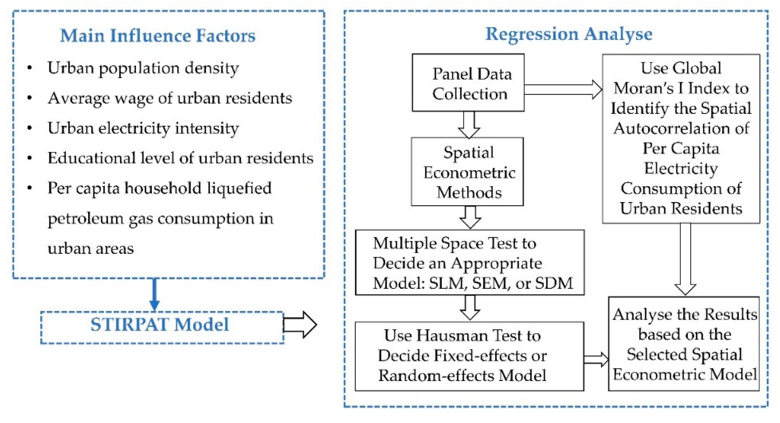
This paper employs the Impact of Population, Affluence and Technology (IPAT) model to identify the effect of the average wage on the per capita electricity consumption of urban residents. This model, however, ignores the effects of other determinants [24]. Therefore, through further improvements to the IPAT model, some scholars have proposed the Stochastic Impacts by Regression on Population, Affluence and Technology (STIRPAT) model. By considering the factors of population, affluence, and technological progress, the model can randomly expand other important factors that affect the environment [25]. This paper uses the STIRPAT model to test the impact of average wage on the per capita electricity consumption of urban residents. Previous studies have used the STIRPAT model to study the driving factors of energy consumption [26]. In order to mitigate the impact of heteroscedasticity, the variables selected in this paper are logarithmic. Accordingly, the STIRPAT model is constructed as follows:
where REC is the per capita electricity consumption of urban residents; WAGE is the average wage of urban residents, denoting the degree of affluence; POP is the urban population density, representing the population factor; EI is the urban electricity intensity, reflecting the technical level; EDU stands for the educational level of urban residents; LPG represents the per capita household liquefied petroleum gas consumption in urban areas; and εit denotes the error term.
Considering the spatial interaction between regional production and the regional interdependence of electric utilities, it seems reasonable that the per capita electricity consumption of urban residents has a spatial correlation in China. Conversely, ignoring the potential spatial correlation of the per capita electricity consumption of urban residents may affect the validity of elasticity estimations and the accurate forecasting of the per capita electricity consumption of urban residents, thereby affecting the achievement of the goal of securing supply in China’s electricity sector. The SDM jointly considers the impacts of spatial lag of the dependent variables and the independent variables [27]. Therefore, in this paper, we established a spatial econometric model for the per capita electricity consumption of urban residents in China based on the STIRPAT model.
Here, i and j represent different cities; Wij is the spatial weight matrix; Xit is the vector of influencing factors; LnRECit is the per capita electricity consumption of urban residents, ; is an intercept term; β is the regression coefficient for the influencing factors; is the spatial autoregressive coefficient for the per capita electricity consumption of urban residents; is the spatial regression coefficient for the influencing factors; λ denotes the spatial regression coefficient of the error term; and εit denotes the error term.
For Equations (6) and (7), if ρ ≠ 0, φ = 0, and λ = 0, then Equation (6) is the SLM, indicating that the per capita electricity consumption of urban residents in one city is affected by that in the neighbouring cities; if λ ≠ 0, ρ = 0 and φ = 0, then Equations (6) and (7) are the SEM, which indicates that the per capita electricity consumption of urban residents in one city is affected by factors other than the average wage of urban residents, urban population density, urban electricity intensity, educational level of urban residents, and the per capita household liquefied petroleum gas consumption in urban areas in neighbouring cities; if ρ ≠ 0, λ = 0 and φ ≠ 0, then Equation (6) is the SDM, which shows that the per capita electricity consumption of urban residents in one city is affected not only by the per capita electricity consumption of urban residents in the neighbouring cities, but also by the average wage of urban residents, urban population density, urban electricity intensity, educational level of urban residents, and the per capita household liquefied petroleum gas consumption in urban areas in the neighbouring cities.
The SDM jointly considers the impacts of the spatial lag of the dependent variables and the independent variables. The use of two Lagrange multiplier tests (i.e., LM_test for no spatial lag and Robust LM_test for no spatial lag; LM_test for no spatial error and Robust LM_test for no spatial error) determines whether the spatial lag effect or the spatial error effect is significant. If one LM test shows a significant effect while the other effect is not significant, this study should adopt the significant form spatial effect model. If the LM test results show that the two effects are significant or not significant simultaneously, this study should adopt the SDM, and, by the Wald or likelihood ratio (LR) test, determine whether the SDM can be simplified into the SLM or SEM. A flowchart summarizing the regression analysis is shown in Figure 1.
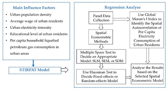
Figure 1.
Flowchart of the regression analysis.
The parameter estimates in the nonspatial model represent the marginal effect, whereas the coefficients in the spatial Durbin model do not. For this purpose, one should use the direct and indirect effect estimates to interpret the model [28]. Meanwhile, one should note that the direct effects of the explanatory variables are different from their coefficient estimates. The direct effect represents the influence of a local independent variable on the local dependent variable. This measure includes feedback effects that arise as a result of impacts passing through adjacent areas (e.g., from region i to j to k) and back to the area that the change originated from (region i). The indirect effect, known as spatial spillover, represents the impact of a local independent variable on the dependent variables in the adjacent areas. The total effect is simply the sum of the direct and indirect effects. LeSage and Pace [28] and Elhorst [29] point out that the indirect effects of the independent variables should be used to examine whether or not spatial spillovers exist. By estimating the direct and indirect effects, the regression model can accurately reflect the marginal effect of explanatory variables. Therefore, this paper mainly observes the impact of average wage on per capita electricity consumption of urban residents through direct and indirect effects.
2.2. Data
2.2.1. Dependent Variable
The per capita electricity consumption of urban residents (REC) refers to the direct household energy consumption of urban residents. The REC was measured by the ratio of urban residential electricity consumption to urban population.
2.2.2. Core independent Variable
The average wage of urban residents (WAGE) effects the amount and structure of household energy consumption [30]. With an increase in the residents’ income, urban residents will buy and use more household appliances and enjoy more powered services, which will lead to an increase in the REC [31]. The residents’ income level was measured based on the average wage of urban residents and converted into the price GDP index in 2005.
2.2.3. Control Variables
Urban population density (POP) is an important factor affecting the per capita electricity consumption of urban residents. However, the total effects of population density on the REC are ambiguous. On the one hand, a higher population density would lead to a higher degree of urbanisation and industrialisation; therefore, the electricity consumption of urban residents may be affected. On the other hand, a high population density makes it possible for power-sharing of residential infrastructure and the intensive use of electricity, thereby reducing the electricity consumption of urban residents, which is beneficial to the environment. To find out which of the two effects prevail, the urban population density was utilised as an additional explanatory variable. The urban population density was measured as a proportion of the urban population to the administrative area.
Urban electricity intensity (EI) was also examined in the present study. Progress in energy technology can change the behaviour of residents [32]. For example, improving the efficiency of household appliances can reduce the REC. However, since progress in energy technology cannot be directly measured, the energy intensity can be used to provide an indirect measure [33,34,35]. Social electricity consumption drives economic growth and societal progress; that is, a decrease in the social electricity consumption per unit of GDP would result in a decline in the electricity intensity, thus reflecting the progress of energy technology. The progress of energy technology was measured by the rate of total urban electricity consumption to GDP.
Per capita household liquefied petroleum gas consumption in urban areas (LPG) was also considered. In general, liquefied petroleum gas and electricity are alternative fuel sources for cooking in Chinese homes, and the REC depends on domestic liquefied petroleum gas consumption. Thus, the per capita household liquefied petroleum gas consumption was calculated based on the ratio of total liquefied petroleum gas consumption in urban households to the number of people using liquefied petroleum gas.
Educational level of urban residents (EDU) has a significant impact on a household’s energy-saving behaviour [36]. Residents with a higher educational level and strong environmental awareness are more likely to actively respond to energy-saving policies and buy energy-saving household appliances, thus reducing resident electricity consumption [37,38,39]. We adopted the ratio of the actual urban education expenditure to urban financial expenditure as the proxy of urban educational level and transformed this variable to a constant 2005 price of RMB [40].
2.3. Data Source
This study utilised a balanced panel data set for 278 of China’s cities for the period 2005–2016. Data regarding these cities were sourced from the China City Statistical Yearbook (2006–2017) and the China Urban Construction Statistical Yearbook (2006–2017). A total of 3336 observations were gathered between 2005 and 2016. All variables were adopted as their natural logarithm for processing potential heteroscedasticity. The variable indicators selected in this study are summarised in Table 1, with the descriptive statistics of the variables listed in Table 2. Each variable changed within the actual range of variation with no extreme outliers. As shown in Table 2, each variable has significant summit and fat-tailed skewed characteristics, in which skewness is not equal to zero and kurtosis exceeds three, showing non-normality characteristics, which was also verified by the Jarque–Bera test. The Variance Inflation Factor (VIF) was employed to test the multi-collinearity of the independent variables. The results in Table 3 show that the maximum value of VIF did not exceed 3, and the minimum value was no less than 0. Its average value was 1.08. Therefore, the independent variables do not exhibit serious multi-collinearity.

Table 1.
Variable description.
Table 2.
Descriptive statistics of variables.
Table 3.
Results of the VIF test.
Before the empirical analysis, it was necessary to identify the stationarity of data by using the panel unit root test. Because the estimation results are meaningful only when the variables used in the regressions are either stationary or integrated of the same order, tests of stationarity should be performed to avoid spurious regressions. The two methods most widely used in a panel root test are LLC and IPS. The main difference between the two test methods is that the LLC assumes that the panel data are homogeneous while IPS allows panel data to be heterogeneous. To ensure that the results of stability testing were robust, both methods for testing were use. The results are provided in Table 4. On the whole, the panel unit root test results indicated that there was no evidence for the existence of a unit root for any of the variables used in the empirical study, as the statistics for all variables in each level were statistically significant. Hence, from Table 4, we can see that the variable data is stable and meets the basic requirements for the establishment of the model.
Table 4.
Results of the unit root test for all variables.
The panel cointegration tests were applied to estimate the existence of the long-run equilibrium relationship among the selected variables. Table 5 presents the results relating to the various tests attributable to Pedroni and Kao. Five statistics (ADF statistic, Panel PP-Statistic, Panel ADF-Statistic, Group PP-Statistic, and Group ADF-Statistic) show a cointegration relationship and allow us to reject the null hypothesis at the 5% or 1% significance levels, indicating the existence of long-term equilibrium relationships among the six variables.
Table 5.
Results of panel cointegration tests.
3. Results
3.1. Visual Analysis
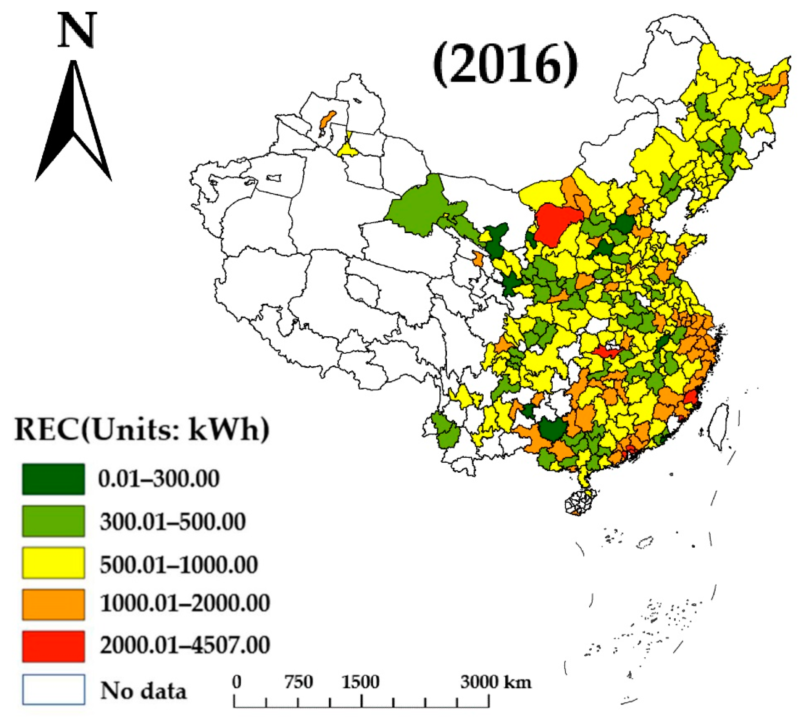
Based on the ArcGIS technology platform, the REC spatial distribution maps of 278 cities in 2005, 2010, and 2016 are shown in Figure 2, Figure 3 and Figure 4, respectively. It can be seen that, from 2005 to 2006, the REC level in China rose rapidly, and the REC within different areas exhibited a large variance and the existence of spatial dependence. Specifically, the REC level in the south-eastern areas was slightly higher than that in the central and western areas, which presents characteristics of spatial agglomeration. From the viewpoint of geography, cities with a high REC were predominantly concentrated in the economically developed cities of China, such as in the Guangdong and Fujian provinces. Therefore, the global Moran’s I index was used to test whether the annual REC in China had spatial autocorrelation characteristics, as described in the following subsections.
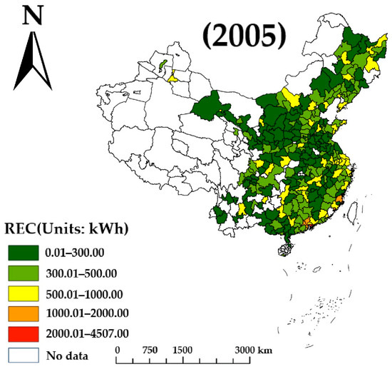
Figure 2.
Spatial pattern evolution of China’s REC in 2005.
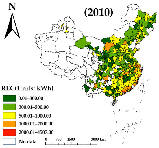
Figure 3.
Spatial pattern evolution of China’s REC in 2010.

Figure 4.
Spatial pattern evolution of China’s REC in 2016.
3.2. Spatial Correlation Analysis
According to the approach above, we calculate the global Moran’s I index of China’s REC from 2005 to 2016, which ranged from 0.159 to 0.272 (see Table 6). As shown in Table 6, the annual global Moran’s I index during the study period passes the significance test at the 1% level. The results indicate that there was relatively significant spatial autocorrelation of REC from 2005 to 2016. Moreover, in general, the annual global Moran’s I indices display an upward trend in the sample period, indicating that the spatial autocorrelation of REC was strengthened.
Table 6.
Global spatial correlation coefficient (Moran’s I).
3.3. Spatial Regression Analysis
The Moran’s I test results discussed above confirmed the spatial dependence of the REC in China. In other words, the REC had spatial spillover effects in China. Therefore, it was essential to establish the spatial economic model.
To determine a suitable spatial economic model, we carried out the (Robust) LM test, the LR test, the Wald test, and the Hausman test (Table 7). The test results showed that both the LM (error) and Robust LM (error) tests were significantly positive at the significance level of 1%, indicating that the residual items of the model were spatially correlated. The results of the LR test and Wald test were significant at the 1% level, denoting that the independent and dependent variables had spatial effects in the model. Therefore, SDM was selected. Additionally, through the Hausman test and LR joint significance test (i.e., space fixed effect or time fixed effect), this study could determine whether the spatial econometric model should adopt a pool fixed effect, space fixed effect, time fixed effect, or space-and-time fixed effect. The Hausman test results suggested that the fixed effect should be selected. We performed the LR joint significance test to investigate the null hypothesis that the spatial effects and time-period effects were jointly insignificant. The null hypothesis that the spatial fixed effects were jointly insignificant was rejected at the 1% significance level (5131.7137, 83 degrees of freedom, p < 0.01). However, the null hypothesis that the time fixed effects were jointly insignificant was not rejected (25.0091, 29 degrees of freedom, p = 0.7487). Thus, these results justified the panel data model with spatial fixed effects. On the basis of the above results, we chose the SDM with a spatial fixed effect to explore the spatial spillover of residents’ income on the REC in China.
Table 7.
Spatial model test results under the economic distance spatial weight matrix.
The parameter estimates in the nonspatial model represent the marginal effect, whereas the coefficients in the SDM do not. For this purpose, one should use the direct effect and indirect effect (spatial spillover effect) to interpret the model. As shown in Table 8, ρ was significant at the 1% level, denoting that the REC had a spatial spillover effect. This was consistent with the global Moran’s I index test results. The SDM estimation results revealed that for every 1% increase in the REC in neighbouring cities, the REC increased by 0.73% in local cities. Table 8 presents the direct effect, indirect effect, and the total effect of the explanatory variables in the SDM under the economic distance spatial weight matrix. Note that we were more interested in explaining the direct and indirect effects of the variables.
Table 8.
Regression results of SDM under the economic distance spatial weight matrix.
For the core explanatory variable, namely the average wage of urban residents, the estimation results provided in Table 8 can be summarised as follows: (1) The direct effect of the local average wage of urban residents on the REC was positive and significant at the 1% level, denoting that the local average wages of urban residents could promote the growth of REC in local cities. (2) The spatial spillover effect of the average wage of urban residents on the REC was positive and significant at the 1% level, denoting that the average wage of urban residents in neighbouring cities had a promoting effect on the REC in local cities. (3) The total effect of the average wage of urban residents was the sum of the direct and indirect effects. Interestingly, the spatial spillover effect of average wages on the REC was greater than the direct effect. This, in turn, implied that the spatial spillover effect of average wages had a greater impact on the REC in China.
For the control variables, the estimation results of the direct effects showed that the urban population density, the per capita household liquefied petroleum gas consumption in urban areas, and the education level of urban residents in local cities had significant inhibitory effects on the REC in local cities. This result also indicates that reducing urban electricity intensity in the local cities is helpful to reduce REC in local cities. Moreover, the urban population density, urban electricity intensity, and education level of urban residents in neighbouring cities had a promoting effect on the REC in the local cities.
3.4. Robustness Analysis
To test the robustness of the SDM evaluation results under the economic distance spatial weight matrix, the inverse distance spatial weight matrix (W_distance) and the four nearest neighbours spatial weight matrix (W_k4) were established. The inverse distance spatial weight matrix (W_distance) was established based on the reciprocal of the distance between the two cities.
Table 9 shows the global Moran’s I value of the REC in China from 2005 to 2016 under the W_distance and W_k4. This table shows that the REC spatial spillover effect was robust. Furthermore, it shows that both the LM (error) and Robust LM (error) tests were significantly positive at the significance level of 1%, indicating that the residual items of the model were spatially correlated under the W_distance and W_k4. Table 10 shows that the results of the LR and the Wald tests were significant at the 1% level under the W_distance and W_k4, indicating that the independent variables and dependent variables of the model have a spatial spillover effect. Based on this, SDM was the better choice for empirical analysis. Meanwhile, the Hausman test results showed that the fixed effect should be selected. Therefore, under the W_distance and W_k4, the SDM with the fixed effect was selected to investigate the spatial spillover effect of residents’ income on the REC in China.
Table 9.
Global Moran’s I value under the W_distance and W_k4.
Table 10.
Spatial models test results under the W_distance and W_k4.
Table 11 and Table 12 show that ρ was significant at the 1% significance level under the W_distance and W_k4, indicating that the REC had a spatial spillover effect in China. Meanwhile, under the W_distance and W_k4, the direct effect and the spatial spillover effect of the average wage had a significant promoting effect on the growth of REC in China, and the spatial spillover effect of the average wage on the REC was greater than the direct effect. Under the W_distance and W_k4, the estimated results of the control variables were similar to those presented in Table 4. These results confirmed that our empirical results were robust.
Table 11.
Regression results of SDM under the W_distance.
Table 12.
Regression results of SDM under the W_k4.
4. Discussion
The spatial spillover effect of residents’ electricity consumption and average wage comes from the interdependence of social and economic activities between neighbouring cities, the similarity of residents’ lifestyle and consumption behaviour, and the flow of the labour force between neighbouring cities [3]. These occur for the following specific reasons. First, the family lifestyle and consumption behaviour in neighbouring cities are similar. That is, residents of one city are influenced by the lifestyle and consumption behaviour of families in neighbouring cities. Residents may imitate the power consumption behaviour of their neighbours, which affects their choice and use of household appliances, and thus results in the spatial correlation of residents’ power consumption. Second, there is movement of labour between neighbouring cities, for example, by people who live in the same city but work in adjacent cities. Third, the spatial correlation of residential electricity consumption comes from the interdependence of social and economic activities between neighbouring cities. For example, residents have a strong economic dependence on what happens in their neighbourhood. In this case, changes in the economic conditions of neighbouring cities will have an impact on the social and economic conditions of local cities, and, in turn, impact the electricity consumption of residents in local cities. Lastly, the implementation of power policies across regions results in a spatial dependence in residents’ electricity consumption between neighbouring cities.
The direct effect of average wages on the REC is significant and positive, indicating that an increase in the residents’ average wages in local cities leads to an increase in the REC in local cities. With an increase in average wages, urban residents are likely to buy more household appliances and enjoy more electricity services, thereby increasing the REC [41,42,43,44]. We wish to stress, emphatically, that compared with the indirect effect of the average wages on the REC, the direct effect of the average wages was relatively small.
Regarding the control variables, we found that the direct effect of urban population density on the REC in China was significant and negative, indicating that an increase in population density in local cities played a positive role in reducing the REC in local cities. The indirect effect (spatial spillover effect) of the population density on the REC was significant and positive, indicating that the increase in the urban population density in the neighbouring cities led to an increase in the REC in local cities.
As shown in Table 8, the direct effect of residents’ education level on the REC in China was significant and negative, indicating that the improvement of the urban residents’ education level in local cities led to a decrease in the REC in local cities. One possible explanation is that residents with a high education level in China might have greater energy conservation awareness and environmental protection behaviours [45]. The education level of the urban residents in China affects residents’ acceptance of renewable energy and the use of energy-saving appliances. Urban residents with a high education level are more likely to purchase energy-saving appliances. However, the indirect effect of the education level on the REC was significant and positive, indicating that the increase in the residents’ education level in the neighbouring cities led to an increase in the REC in the local cities.
From the perspective of the per capita household liquefied petroleum gas consumption in urban areas, the direct effect was very significant and negative, which showed that the decrease in the per capita household liquefied petroleum gas consumption in urban areas in local cities led to an increase in the REC in local cities. The reason for this is that liquefied petroleum gas and electricity are alternative cooking fuels in China. During 2005–2016, with the decrease in the per capita household liquefied petroleum gas consumption in urban areas, the REC increased in China. However, the indirect effect of the per capita household liquefied petroleum gas consumption on the REC was not significant.
Finally, we focused on the urban electricity intensity. The direct effect of the electricity intensity on the REC was positive and significant, which indicated that the decrease in the urban electricity intensity in local cities resulted in a decrease in the REC in local cities. Compared with the other variables, the elasticity coefficient of the electricity intensity to the REC was the largest, which showed that reducing the electricity intensity was the most important factor in reducing the REC. The decrease in urban electricity intensity may be largely related to the gradual maturity of the technology used in energy-saving household appliances in China and greater marketing efforts in favour of energy-saving household appliances [46]. Meanwhile, the indirect effect of the electricity intensity on the REC was significant and positive, indicating that increases in the electricity intensity in the neighbouring cities led to an increase in the REC in local cities.
5. Conclusions and Policy Recommendations
In this paper, we studied the temporal–spatial patterns of the REC based on the ArcGIS technology platform. We tested the spatial autocorrelation (spatial spillover effect) of REC by using the global Moran’s I index. Based on the results of the Wald test and LR test, the SDM was applied to identify the direct and spatial spillover effect of the residents’ income on the REC in China over the study period, from 2005 to 2016. Several novel findings were presented in this paper, and can be summarised as follows:
First, the REC level in China rose rapidly from 2005 to 2006, and showed large variance between different areas. Specifically, the REC level in south-eastern areas was slightly higher than that in the central and western areas. Second, the REC in China presented an obvious spatial spillover effect. The global Moran’s I index value of the REC over the study period reflected an upward trend for the spatial spillover effect. Third, the spatial spillover effect of residents’ income was greater than the direct effect. The spatial spillover effect of residents’ income was an important determinant of REC growth in China. In addition, we verified the impact of the urban population density, urban electricity intensity, education level of urban residents, and the per capita household liquefied petroleum gas consumption on the REC. The results showed that reducing the urban electricity intensity helps reduce residential electricity consumption, in line with the findings of international and local literature.
Based on the findings reported in this paper, we propose policy recommendations in the following aspects:
First, this paper established an SDM model that shows the importance of considering the spatial spillover effect on the REC and residents’ average wages to model the electricity consumption for the Chinese household sector. Omitting spatial interactions leads to a bias in the models used by the Chinese electricity sector. The bias in the estimated parameters generates wasted energy and environmental resources and increases the probability of blackouts, which in turn decreases the profits of the Chinese electricity sector. Hence, accurate electricity consumption forecasting is paramount for decision-making in the Chinese electricity sector. The SDM model established here can not only improve the forecasting accuracy of electricity consumption in China’s household sector but also help the Chinese electricity sector to make strong investment and planning decisions.
Second, the development over time and space of distributed generation systems and intermittent renewable energy will facilitate geographic de-concentration in the Chinese electricity sector. Therefore, the spatial econometric model will gain importance in modelling the electricity markets and will be paramount to achieving the goals of electricity supply security in the Chinese electricity sector.
Third, the model estimated the spatial spillover effect of average wages. The results showed that the spatial spillover effect of the average wage has a larger effect on the REC than the direct effect of the average wage, which extends the findings of the international and local literature. This paper verified the spatial spillover effect of residential electricity consumption, which provides a theoretical basis for promoting the development of electricity integration in China. Hence, when policymakers formulate electricity policies for the household sector, both local cities and surrounding cities need to be considered.
Lastly, the models presented in this paper could be particularly useful in other areas of the Chinese electricity sector. For example, considering China’s hydropower resources, the proposed models can be used to improve wind and solar power forecasting that are of enormous importance to the supply of energy in China. However, due to the spatial heterogeneity and complexity of urban residents’ electricity consumption, our future research will apply the exponent of cross-sectional dependence of Bailey et al. [47] and the multilevel dynamic factor model proposed by Choi et al. [48], Ergemen and Rodríguez-Caballero [49], Breitung and Eickmeier [50], and Rodríguez-Caballero [51] to further investigate the relationship between average wages and the REC in China.
Author Contributions
Conceptualisation, S.L. and Z.Z.; methodology, S.L.; software, S.L.; validation, S.L.; formal analysis, S.L.; investigation, S.L.; resources, Z.Z.; data curation, S.L.; writing—original draft preparation, S.L.; writing—review and editing, S.L. and Z.Z.; visualisation, J.Y.; supervision, Z.Z.; project administration, W.H. and J.Y.; funding acquisition, W.H. and Z.Z. All authors have read and agreed to the published version of the manuscript.
Funding
This research was funded by the National Natural Science Foundation of China (Grant No. 42071085), the Open Project of the State Key Laboratory of Cryospheric Science (Grant No. SKLCS 2020-10), the National Nature Science Foundation of China (Grant No. 41701087), and the National Social Science Foundation (Grant No. 19BGL003).
Institutional Review Board Statement
Not applicable.
Informed Consent Statement
Not applicable.
Data Availability Statement
Not applicable.
Conflicts of Interest
The authors declare no conflict of interest.
References
- Zhu, X.; Li, L.; Zhou, K.; Zhang, X.; Yang, S. A meta-analysis on the price elasticity and income elasticity of residential electricity demand. J. Clean. Prod. 2018, 201, 169–177. [Google Scholar] [CrossRef]
- de Assis Cabral, J.; de Freitas Cabral, M.V.; Júnior, A.O.P. Elasticity estimation and forecasting: An analysis of residential electricity demand in Brazil. Util. Pol. 2020, 66, 101108. [Google Scholar] [CrossRef]
- Zhao, X.-G.; Li, P.-L. Is the energy efficiency improvement conducive to the saving of residential electricity consumption in China? J. Clean. Prod. 2020, 249, 119339. [Google Scholar] [CrossRef]
- Boogen, N.; Datta, S.; Filippini, M. Dynamic models of residential electricity demand: Evidence from Switzerland. Energy Strategy Rev. 2017, 18, 85–92. [Google Scholar] [CrossRef] [Green Version]
- Holz, F.; Karakosta, C.; Neumann, A. The challenges of spatial and temporal aggregation: Modelling issues, applications, and policy implications. Util. Pol. 2020, 62, 100993. [Google Scholar] [CrossRef]
- Bridge, G. The map is not the territory: A sympathetic critique of energy research’s spatial turn. Energy Res. Soc. Sci. 2018, 36, 11–20. [Google Scholar] [CrossRef] [Green Version]
- Noonan, D.S.; Hsieh, L.-H.C.; Matisoff, D. Spatial effects in energy-efficient residential HVAC technology adoption. Environ. Behav. 2013, 45, 476–503. [Google Scholar] [CrossRef] [Green Version]
- Gomez, L.M.B.; Filippini, M.; Heimsch, F. Regional impact of changes in disposable income on Spanish electricity demand: A spatial econometric analysis. Energy Econ. 2013, 40, S58–S66. [Google Scholar] [CrossRef]
- Cho, S.-H.; Kim, T.; Kim, H.J.; Park, K.; Roberts, R.K. Regionally-varying and regionally-uniform electricity pricing policies compared across four usage categories. Energy Econ. 2015, 49, 182–191. [Google Scholar] [CrossRef]
- de Assis Cabral, J.; Legey, L.F.L.; Freitas Cabral, M.V.D. Electricity consumption forecasting in Brazil: A spatial econometrics approach. Energy 2017, 126, 124–131. [Google Scholar] [CrossRef]
- Ohtsuka, Y.; Oga, T.; Kakamu, K. Forecasting electricity demand in Japan: A Bayesian spatial autoregressive ARMA approach. Comput. Stat. Data Anal. 2010, 54, 2721–2735. [Google Scholar] [CrossRef]
- Ohtsuka, Y.; Kakamu, K. Space-time model versus VAR model: Forecasting electricity demand in Japan. J. Forecast. 2013, 32, 75–85. [Google Scholar] [CrossRef]
- Akarsu, G. Analysis of regional electricity demand for Turkey. Reg. Stud. Reg. Sci. 2017, 4, 32–41. [Google Scholar] [CrossRef]
- Wang, S.; Liu, Y.; Zhao, C.; Pu, H. Residential energy consumption and its linkages with life expectancy in mainland China: A geographically weighted regression approach and energy-ladder-based perspective. Energy 2019, 177, 347–357. [Google Scholar] [CrossRef]
- Wang, S.; Zhao, C.; Liu, H.B.; Tian, X.L. Exploring the spatial spillover effects of low-grade coal consumption and influencing factors in China. Resour. Policy 2021, 70, 101906. [Google Scholar] [CrossRef]
- De Siano, R.; Sapio, A. Spatial Econometrics in Electricity Markets Research. In Handbook of Energy Finance: Theories. Practices and Simulations; Goutte, S., Nguyen, D.K., Eds.; World Scientific Publishing: Singapore, 2020; pp. 121–156. [Google Scholar]
- Elhorst, J.P. Specification and estimation of spatial panel data models. Int. Reg. Sci. Rev. 2003, 26, 244–268. [Google Scholar] [CrossRef]
- Messner, S.F.; Anselin, L.; Baller, R.D.; Hawkins, D.F.; Deane, G.; Tolnay, S.E. The spatial patterning of county homicide rates: An application of exploratory spatial data analysis. J. Quant. Criminol. 1999, 15, 423–450. [Google Scholar] [CrossRef]
- Anselin, L. Local indicators of spatial association-LISA. Geogr. Anal. 1995, 27, 93–115. [Google Scholar] [CrossRef]
- Moran, P.A.P. The interpretation of statistical maps. J. R. Stat. Soc. Ser. B Stat. Methodol. 1948, 10, 243–251. [Google Scholar] [CrossRef]
- Cheng, Z.H.; Li, L.S.; Liu, J. The emissions reduction effect and technical progress effect of environmental regulation policy tools. J. Clean. Prod. 2017, 149, 191–205. [Google Scholar] [CrossRef]
- Liu, Q.Q.; Wang, S.J.; Zhang, W.Z.; Zhan, D.S.; Li, J.M. Does foreign direct investment affect environmental pollution in China’s cities? A spatial econometric perspective. Sci. Total Environ. 2018, 613–614, 521–529. [Google Scholar] [CrossRef] [PubMed]
- Tian, Y.; Sun, C.W. Comprehensive carrying capacity, economic growth and the sustainable development of urban areas: A case study of the Yangtze River Economic Belt. J. Clean. Prod. 2018, 195, 486–496. [Google Scholar] [CrossRef]
- Ehrlich, P.R.; Holdren, J.P. Impact of population growth. Science 1971, 171, 1212–1217. [Google Scholar] [CrossRef] [PubMed]
- Dietz, T.; Rosa, E.A. Rethinking the environmental impacts of population, affluence and technology. Hum. Ecol. Rev. 1994, 1, 277–300. [Google Scholar]
- Xu, B.; Lin, B. Regional differences of pollution emissions in China: Contributing factors and mitigation strategies. J. Clean. Prod. 2016, 112, 1454–1463. [Google Scholar] [CrossRef]
- Yang, T.C. Introduction to spatial econometrics. Spat. Demogr. 2013, 1, 143–145. [Google Scholar] [CrossRef] [Green Version]
- LeSage, J.; Pace, R.K. Introduction to Spatial Econometrics; Chapman and Hall/CRC: New York, NY, USA, 2009. [Google Scholar]
- Elhorst, J.P. Spatial Panel Data Models. In Handbook of Applied Spatial Analysis; Fischer, M.M., Getis, A., Eds.; Springer: New York, NY, USA, 2013; pp. 37–93. [Google Scholar]
- Brandon, G.; Lewis, A. Reducing household energy consumption: A qualitative and quantitative field study. J. Environ. Psychol. 1999, 19, 75–85. [Google Scholar] [CrossRef]
- Su, Y.W. Residential electricity demand in Taiwan: Consumption behavior and rebound effect. Energy Policy 2019, 124, 36–45. [Google Scholar] [CrossRef]
- Hondo, H.; Baba, K. Socio-psychological impacts of the introduction of energy technologies: Change in environmental behavior of households with photovoltaic systems. Appl. Energy 2010, 87, 229–235. [Google Scholar] [CrossRef]
- Song, M.; Guo, X.; Wu, K.; Wang, G. Driving effect analysis of energy consumption carbon emissions in the Yangtze River Delta region. J. Clean. Prod. 2015, 103, 620–628. [Google Scholar] [CrossRef]
- Liu, Y.; Chen, Z.M.; Xiao, H.; Yang, W.; Liu, D.; Chen, B. Driving factors of carbon dioxide emissions in China: An empirical study using 2006–2010 provincial data. Front. Earth Sci. 2017, 11, 156–161. [Google Scholar] [CrossRef]
- Zhang, J.; Chang, Y.; Zhang, L.; Li, D. Do technological innovations promote urban green development?—A spatial econometric analysis of 105 cities in China. J. Clean. Prod. 2018, 182, 395–403. [Google Scholar] [CrossRef]
- Poortinga, W.; Steg, L.; Vlek, C.; Wiersma, G. Household preferences for energy-saving measures: A conjoint analysis. J. Econ. Psychol. 2003, 24, 49–64. [Google Scholar] [CrossRef]
- Steg, L. Promoting household energy conservation. Energ. Policy 2008, 36, 4449–4453. [Google Scholar] [CrossRef]
- Bekker, M.J.; Cumming, T.D.; Osborne, N.K.; Bruining, A.M.; McClean, J.I.; Leland, L.S. Encouraging electricity savings in a university residential hall through a combination of feedback, visual prompts, and incentives. J. Appl. Behav. Anal. 2010, 43, 327–331. [Google Scholar] [CrossRef]
- Thøgersen, J.; Grønhøj, A. Electricity saving in households—A social cognitive approach. Energy Policy 2010, 38, 7732–7743. [Google Scholar] [CrossRef]
- Que, W.; Zhang, Y.; Schulze, G. Is public spending behavior important for Chinese official promotion? Evidence from city-level. China Econ. Rev. 2019, 54, 403–417. [Google Scholar] [CrossRef]
- Zacarias-Farah, A.; Geyer-Allély, E. Household consumption patterns in OECD countries: Trends and figures. J. Clean. Prod. 2003, 11, 819–827. [Google Scholar] [CrossRef]
- Yohanis, Y.G.; Mondol, J.D.; Wright, A.; Norton, B. Real-life energy use in the UK:How occupancy and dwelling characteristics affect domestic electricity use. Energy Build. 2008, 40, 1053–1059. [Google Scholar] [CrossRef]
- McLoughlin, F.; Duffy, A.; Conlon, M. Characterising domestic electricity consumption patterns by dwelling and occupant socio-economic variables: An Irish case study. Energy Build. 2012, 48, 240–248. [Google Scholar] [CrossRef] [Green Version]
- Damari, Y.; Kissinger, M. An integrated analysis of households’ electricity consumption in Israel. Energy Policy 2018, 119, 51–58. [Google Scholar] [CrossRef]
- Leahy, E.; Lyons, S. Energy use and appliance ownership in Ireland. Energy Policy 2010, 38, 4265–4279. [Google Scholar] [CrossRef] [Green Version]
- Andrews-Speed, P.; Ma, G. Household Energy Saving in China: The Challenge of Changing Behaviour; Springer: Singapore, 2016; pp. 22–39. [Google Scholar]
- Bailey, N.; Kapetanios, G.; Pesaran, M.H. Exponent of Cross-sectional Dependence: Estimation and Inference. J. Appl. Econ. 2016, 31, 929–960. [Google Scholar] [CrossRef] [Green Version]
- Choi, I.; Kim, D.; Kim, Y.J.; Kwark, N.S. A multilevel factor model: Identification, asymptotic theory and applications. J. Appl. Econ. 2018, 33, 355–377. [Google Scholar] [CrossRef]
- Ergemen, Y.E.; Rodríguez-Caballero, C.V. Estimation of a dynamic multilevel factor model with possible long-range dependence. Int. J. Forecast. 2022. [Google Scholar] [CrossRef]
- Breitung, J.; Eickmeier, S. Analyzing international business and financial cycles using multilevel factor models: A comparison of alternative approaches. Adv. Econ. 2016, 35, 177–214. [Google Scholar] [CrossRef]
- Rodríguez-Caballero, C.V. Energy consumption and GDP: A panel data analysis with multi-level cross-sectional dependence. Econ. Stat. 2022, 23, 128–146. [Google Scholar] [CrossRef]


Publisher’s Note: MDPI stays neutral with regard to jurisdictional claims in published maps and institutional affiliations. |
© 2022 by the authors. Licensee MDPI, Basel, Switzerland. This article is an open access article distributed under the terms and conditions of the Creative Commons Attribution (CC BY) license (https://creativecommons.org/licenses/by/4.0/).