Film Boiling Conjugate Heat Transfer during Immersion Quenching

Abstract

Boiling conjugate heat transfer is an active field of research encountered in several industries, including metallurgy, power generation and electronics. This paper presents a computational fluid dynamics approach capable of accurately modelling the heat transfer and flow phenomena during immersion quenching: a process in which a hot solid is immersed into a liquid, leading to sudden boiling at the solid–liquid interface. The adopted methodology allows us to couple solid and fluid regions with very different physics, using partitioned coupling. The energy equation describes the solid, while the Eulerian two-fluid modelling approach governs the fluid’s behaviour. We focus on a film boiling heat transfer regime, yet also consider natural convection, nucleate and transition boiling. A detailed overview of the methodology is given, including an analytical description of the conjugate heat transfer between all three phases. The latter leads to the derivation of a fluid temperature and Biot number, considering both fluid phases. These are then employed to assess the solver’s behaviour. In comparison with previous research, additional heat transfer regimes, extra interfacial forces and separate energy equations for each fluid phase, including phase change at their interface, are employed. Finally, the validation of the computational approach is conducted against published experimental and numerical results.

1. Introduction

Boiling conjugate heat transfer can be encountered in multiple applications such as nuclear fission [1], nuclear fusion [2], electronics cooling [3] and metal manufacturing [4]. Our research is motivated by a metallurgical process termed immersion quenching [4], yet is not limited to it. For example, quenching can occur during the chill-down of cryogenic liquid transfer systems and in nuclear reactors and superconductors under accidental conditions [5].

Immersion quenching is an extensively utilised metallurgical process commonly employed to control steel and alloy workpieces’ microstructure to improve their properties. Initially, a metallic sample heats up to 1000 °C, depending on the material. Then it is cooled by submerging it in a coolant. This article focuses only on the usage of water. However, the framework might be adapted to other coolants by choosing relevant heat transfer models. The high solid temperature results in various types of boiling and related heat transfer regimes (HTRs), which change as the cooling process progresses. We consider the complete range of HTRs: film boiling, transition boiling, nucleate boiling, and finally, convective heat transfer. The existence of a particular HTR depends on various parameters, including but not limited to sample wall temperature, coolant temperature, sample geometry, and material properties.

Inadequate cooling can cause samples to distort and crack, resulting from thermal stress developed due to significant temperature gradients [4]. Despite the fact that there have been several research papers dedicated to computational techniques for immersion quenching [6,7,8,9,10,11,12,13,14,15,16,17,18], improvements are still necessary. The manufacturing industry would greatly benefit from a well-functioning, accurate, and efficient computational technique that predicts the temperature profile of the solid during the quenching process and the resulting mechanical stresses. This would enable designs of quenching processes tailored to achieve specific engineering requirements.

Below, we summarise previous research findings and then concentrate on our contribution. The majority of previous publications have used AVL FIRE, a commercial simulation software specialised in internal combustion and components for electrified power trains [19]. Wang et al. [6,7] introduced the immersion quenching computational methodology in AVL FIRE. They solved a conjugate heat transfer problem between solid and fluid regions by assessing the interface temperature and heat transfer coefficient. An energy equation governed the solid region. Meanwhile, the Eulerian two-fluid model (ETF) described the fluid behaviour using a separate set of continuity and momentum equations for each phase completed with a mixture energy equation. In addition, the authors assumed gas-phase, lumping vapour and air together, which decreased computational needs. Nevertheless, HTRs were taken into account, limited to film and nucleate boiling. It should be pointed out that the term of the nucleate boiling mass source was estimated based on a simplistic assumption where the film boiling mass source was multiplied by 100.

Subsequent studies heavily relied on and extended the initial AVL FIRE publications. Srinivasan et al. [8,9] introduced a new approach for modelling the solid–fluid interface, implemented the transition boiling HTR, modified the drag force equation and did not consider the nucleate boiling HTR. They validated their results against a trapezoidal block sample and an aluminium alloy engine cylinder. Greif et al. [10] continued the work and combined the procedure with a structural mechanics analysis in ABAQUS [20]. The quenching of an engine cylinder head was also performed in subsequent work by Jan et al. [11]. Later on, the variable Leidenfrost temperature, lift and wall lubrication interfacial momentum forces were taken into account by Kopun et al. [12,13].

Further work with AVL FIRE considered separate energy equations for gas and liquid phases [14]. Nonetheless, the thermal homogeneous assumption was applied, with the interfacial phase heat transfer coefficient set to a very high value which homogenised the equations. The latest research papers using AVL FIRE discussed the influence and calibration of various coefficients and values within the heat transfer framework, which usually need to be chosen and tuned to achieve valid results [15,16].

Excluding the work conducted with AVL FIRE, there have been two other attempts to numerically simulate the metallurgical process of quenching. The first used the mixture model and bubble crowding method in Fluent, allowing vaporisation and recondensation [17]. The second utilised the Finite Element–Galerkin method with monolithic coupling, tracking the liquid–vapour interface using the Level Set method and anisotropic mesh adaptation [18]. Compared with the ETF methodology, the latter approach uses only one set of Navier-Stokes equations but requires mixing laws. A lower number of governing equations offsets the necessity to resolve the liquid–vapour interface and the repetitive mesh generation. A monolithic approach prevents stability issues at the solid–fluid interface and proves to be often more efficient, yet it aggravates the governing equation implementation because the solid and fluid regions need to be described as a single system [21]. In addition, in Khalloufi’s approach there was only an interfacial phase change, omitting the wall boiling used in the ETF approach and leading to the necessity to introduce an initial, and sometimes artificial, liquid–vapour interface for the phase change to occur. Due to the temperature range and well-presented data, the experimental and numerical results provided in the Khalloufi et al. [18] paper serve as validation data for our computational methodology.

Overall, the scientific work done is quite extensive, but success varies. Immersion quenching is a highly complex process with many physical phenomena co-occurring, some of which have not been fully understood yet. Furthermore, current numerical studies are not always easy to reproduce. This is often due to missing information, such as sample geometries, thermocouple locations, Leidenfrost temperature, and bubble diameter.

This paper is devoted to a computational fluid dynamics methodology during immersion quenching and the understanding of the involved physical phenomena while accounting for the metallic workpiece’s presence via conjugate heat transfer. We do not reckon for microstructure changes within the metallic sample, because this is outwith the scope of this paper.

We attempt to push state-of-the-art heat transfer simulation forward in the framework of the open-source toolbox OpenFOAM [22] blending various versions starting with v1906 released by OpenCFD Ltd. The core methodology is comparable to AVL FIRE, yet with the following differences and/or additions. Firstly, we introduce the nucleate boiling HTR using the Rensselaer Polytechnic Institute (RPI) mechanistic model [23] implemented similarly to Peltola et al. [24] and adapted to the transition and film boiling heat transfer regimes [9]. Moreover, we consider natural convection using the method of Jayatilleke [25], applied to both fluid phases. Interfacial terms account for phase inversion, and additional interfacial forces, virtual mass and turbulence dispersion, are modelled. We solve separate energy equations for gas and liquid and illustrate the effect of liquid–vapour interfacial boiling and condensation. Together with the methodological changes, we perform a theoretical analysis of conjugate heat transfer into boiling fluid resulting in two variables suitable for computational results analysis and assessment. We also provide guidelines throughout the text on how to numerically solve such problems accurately and highlight potential areas that can lead to numerical instabilities.

We validate our methodology, and specifically the film boiling HTR, against a submerged plate made of Inconel 718 alloy at 880 °C [18], where boiling at horizontal surfaces is dominant. We focus on the temperature range between 880 °C and 200 °C, measured at the plate centre. In this range, the film boiling is the dominant HTR. Yet, we also examine plate edges and corners characterised by faster cooling, therefore experiencing all possible HTRs. That supplies an opportunity to carefully study the solver behaviour before proceeding to more complex problems. We also want to highlight here that all previous numerical studies were carried out from the initial temperature of about 500 °C except for Krause et al. [17], whose research is limited to values around 727 °C, still considerably lower than the one studied here.

2. Methodology

Below, we describe the methodology, including governing equations and interfacial terms. The solid–fluid interface and wall boiling modelling are discussed in Section 3. The computational domain consists of two regions. These are solved using the partitioned approach and interact only via temperature boundary conditions. That allows the usage of dedicated solvers for each region to cope with complex physics.

2.1. Governing Equations

We attempt to resolve a three-phase problem consisting of a non-deformable solid, governed by the heat equation, and a two-phase fluid described using two sets of Navier–Stokes equations and a turbulence model. Realistically we could also account for the air as a distinct phase. Nevertheless, we consider the air to have identical properties with water vapour, as have been done in many previous studies without a lack of generality or accuracy [6,7,8,9,10,11,12,13,14,15,16].

2.1.1. Fluid Region

The ETF method employs separate conservation equations governing each fluid phase, and the interfacial models accounting for their interaction. The phases penetrate each other and are represented by volume fractions, which result from their transport equations. Thus, the methodology describes the fluid region without resolving the interface between liquid and vapour, while turbulence equations close the system of equations.

The fluid conservation equations applied to both phases are the following:

Mass conservation

$$\frac{\partial {\alpha }_j{\rho }_j}{\partial t}+\nabla ·\left({\alpha }_j{\rho }_j{\mathit{u}}_j\right)={\dot{m}}_{jk},$$

(1)

where $\alpha$, $\rho$, t and $\mathit{u}$ are volume fraction, density, time, and velocity, respectively, and the subscripts j and k stand either for $L-liquid$ or $V-vapour$, but $j\ne k$. Moreover, $\dot{m}$ is the mass source/sink accounting for the phase change:

$${\dot{m}}_{jk}={\dot{m}}_{w,jk}+{\dot{m}}_{i,jk},$$

(2)

where we recognise two different phase change sources: phase change due to wall boiling ${\dot{m}}_w$ (Section 3.1) and interfacial phase change ${\dot{m}}_i$ (Section 2.2.3). Naturally, the latter term equals to zero if no interfacial phase change (IPC) is activated.

Similarly, the conservation of momentum is given by:

$$\frac{\partial {\alpha }_j{\rho }_j{\mathit{u}}_j}{\partial t}+\nabla ·\left({\alpha }_j{\rho }_j{\mathit{u}}_j{\mathit{u}}_j\right)=-{\alpha }_j\nabla p+\Delta \left({\alpha }_j{\nu }_{eff,j}{\mathit{u}}_j\right)+{\alpha }_j{\rho }_j\mathit{g}-{\alpha }_k({\rho }_j-{\rho }_k)\mathit{g}+({\dot{m}}_{jk}{\mathit{u}}_k-{\dot{m}}_{kj}{\mathit{u}}_j)+F_{jk},$$

(3)

where p denotes the pressure field, which is common for both fluid phases, $\mathit{g}$ stands for the acceleration due to gravity, and ${\nu }_{eff}$ is the effective viscosity ${\nu }_{eff,j}={\nu }_{m,j}+{\nu }_{tr,j}$, where ${\nu }_m$ is the kinematic viscosity, and ${\nu }_{tr}$ is the turbulent viscosity. $F_{jk}$ denotes the influence of interfacial forces dictated by the fluid phases momentum interaction (Section 2.2.1).

Following on, the conservation of energy in the form of specific enthalpy can be written as:

$$\begin{gathered} \frac{\partial {\alpha }_j{\rho }_j{h}_j}{\partial t}+\nabla ·\left({\alpha }_j{\rho }_j{h}_j{\mathit{u}}_j\right)+\frac{\partial {\alpha }_j{\rho }_j{K}_j}{\partial t}+\nabla ·\left({\alpha }_j{\rho }_j{K}_j{\mathit{u}}_j\right)-\Delta \left({\alpha }_j{\gamma }_{eff,j}{h}_j\right)= \\ {\alpha }_j{\rho }_j({\mathit{u}}_j·\mathit{g})+H_j(T_f-T_j)+({\dot{m}}_{jk}{h}_k-{\dot{m}}_{kj}{h}_j)+({\dot{m}}_{jk}{K}_k-{\dot{m}}_{kj}{K}_j), \end{gathered}$$

(4)

where h and T represent specific enthalpy and temperature; $K_j=\frac{1}{2}{\left|{\mathit{u}}_j\right|}^2$, and ${\gamma }_{eff}$ is the effective thermal diffusivity ${\gamma }_{eff,j}={\gamma }_{m,j}+{\gamma }_{tr,j}$ with ${\gamma }_m$, ${\gamma }_{tr}$ standing for molecular thermal diffusivity and turbulent thermal diffusivity, respectively. H is a product of the interfacial area concentration ($A_{ic}=\frac{6{\alpha }_d}{D_d}$) and the heat transfer coefficient calculated following correlations estimating the Nusselt number (Section 2.2.2). Subscripts d and c denote dispersed and continuous phase, respectively, while D is the phase particle diameter. Finally, $T_f$ is the liquid–vapour interface temperature,

$$T_f=\frac{H_L}{H_L+H_V}{T}_L+\frac{H_V}{H_L+H_V}{T}_V+\frac{{\dot{m}}_i\psi }{H_L+H_V},$$

(5)

where $\psi$ is the latent heat. The third term on the RHS disappears when no IPC is allowed.

We also take into account turbulence generated due to the presence of bubbles [26] through the use of the fluid phases mixture $k-ϵ$ model [27]. This effect depends on various factors such as heat transfer regime, coolant subcooling, and geometry, to name a few. In the current work, it is considered for three reasons: the appearance of various heat transfer regimes, although with different impacts on the validation data; the investigation of the IPC (Section 4.3), which substantially reduces the subcooling effect; and the fact that this study is only a predecessor to more complex problems. Here, we introduce the mixture turbulent kinetic energy $k_{mx}$ transport equation:

$$\frac{\partial k_{mx}}{\partial t}+\nabla ·\left({\mathit{u}}_{mx}{k}_{mx}\right)-\Delta \left({\nu }_{tr,mx}{k}_{mx}\right)=G_{mx}-\frac{2}{3}{k}_{mx}\nabla ·{\mathit{u}}_{mx}-{ϵ}_{mx}+G_b\frac{1}{{\rho }_{mx}},$$

(6)

where the subscript $mx$ stands for a mixture of the fluid phases; $G_{mx}$ is the mixture turbulence production, and $G_b$ is the turbulence generation due to bubble presence. Then we also include the transport equation for the dissipation rate of the turbulent kinetic energy mixture ${ϵ}_{mx}$ as:

$$\frac{\partial {ϵ}_{mx}}{\partial t}+\nabla ·\left({\mathit{u}}_{mx}{ϵ}_{mx}\right)-\Delta \left(\frac{{\nu }_{tr,mx}}{{\sigma }_{ϵ}}{ϵ}_{mx}\right)=C_1{G}_{mx}\frac{{ϵ}_{mx}}{k_{mx}}-\frac{2}{3}{C}_1{ϵ}_{mx}\nabla ·{\mathit{u}}_{mx}-C_2\frac{{ϵ}_{mx}^2}{k_{mx}}+C_3{G}_b\frac{{ϵ}_{mx}}{{\rho }_{mx}{k}_{mx}},$$

(7)

where the model constants are ${\sigma }_{ϵ}=1.3$, $C_1=1.44$, $C_2=C_3=1.92$ [28,29].

Finally, the phase continuity equation obeying ${\alpha }_L+{\alpha }_V=1$ is derived from a form developed by Weller [30] following the need for a conservative and bounded equation:

$$\frac{\partial {\alpha }_V}{\partial t}+\nabla ·\left({\mathit{u}}_{tot}{\alpha }_V\right)+\nabla ·\left({\mathit{u}}_r{\alpha }_V(1-{\alpha }_V)\right)={\alpha }_{V}Sp+Su,$$

(8)

where ${\mathit{u}}_{tot}$ and ${\mathit{u}}_r$ are the total and relative velocities of the fluid phases. While $Sp$ and $Su$ are source terms related to dilatation rates accounting for the pressure equation’s compressible part and mass transfer between the fluid phases. Equation (8) is further utilised in a form developed by Rusche [31] to account for turbulent dispersion.

2.1.2. Solid Region

The only necessary equation to solve in the solid region is energy conservation, through a Laplace equation with the temporal term in the specific enthalpy form:

$$\frac{\partial {\rho }_S{h}_S}{\partial t}-\Delta \left({\gamma }_S{h}_S\right)=0.$$

(9)

The subscript S stands for the solid region, while $\gamma$ is the thermal diffusivity defined as ${\gamma }_S=\frac{{\kappa }_S}{c_{p,S}}$, where $\kappa$ stands for the thermal conductivity and $c_p$ represents the isobaric specific heat capacity.

2.2. Interfacial Terms

Due to the usage of the ETF method, we must model the fluid phases interactions. That applies to all governing equations, thus to the continuity, momentum and energy. Both fluid phases can occur in dispersed or continuous states because various two-phase flow regimes can happen. Nevertheless, we do not account for segregated flow. Regardless of the actual flow regime of a particular phase, we utilise interfacial models for continuous and dispersed flows for each phase at every cell and timestep of the simulation and blend them using a weighting function.

$$X_k=w_{c,k}{X}_{c,k}+(1-w_{c,k})X_{d,k},$$

(10)

where X stands for various coefficients/forces depending on the interfacial term of interest and w is the weighting value following piecewise linear approximation:

$$w_{c,k}=min\left(max\left(\frac{{\alpha }_k-{\alpha }_{pc}}{{\alpha }_{fc}-{\alpha }_{pc}},0\right),1\right),$$

(11)

where ${\alpha }_{pc}$ represents the minimum volume fraction to become partially continuous under which $w_{c,k}=0$ and ${\alpha }_{fc}$ represent the minimum volume fraction to become fully continuous, above which $w_{c,k}=1$. Their values are different for momentum and heat transfer interfacial terms.

To calculate the interfacial terms, we also need the bubble/droplet Sauter mean diameter, which is previously used in the literature related to subcooled boiling [28,32,33] and is the default choice to represent a bubble size in OpenFOAM. Nevertheless, due to reasons explained below in detail, we consider the influence of particles’ diameters out of this article’s scope. Their values were chosen to comply with the experimental temperature results, thus used instead as a solution parameter. Throughout the research, we assume the bubble diameter to be 3 mm at atmospheric pressure, subjected to pressure changes but no thermal expansion, coalescence, breakup or bubble crowding. In contrast, the droplet diameter is constant at 0.45 mm. We are aware that bubble dynamics may play a significant role. An alternative would be to use correlations [34] or a more complex approach such as Interfacial Area Transport Equation [35] or Population Balance [28]. Nevertheless, particular bubble dynamics approaches were developed/tested for specific conditions such as subcooling, pressure, heat transfer regime and forced flow. Moreover, the validation problem includes considerable boiling on the horizontal faces, potentially leading to large bubbles if the IPC is not allowed, and to violation of the ETF fundamental assumption. The latter states that the dispersed particle Sauter mean diameter should not exceed the smallest dimension of a control volume (CoV) it is present in (more in Section 4.2). That can result in numerical instability or a need to coarsen the mesh beyond the level needed to resolve the flow dynamics.

2.2.1. Momentum

Multiple forces can arise as a result of phase interaction. We consider drag ${\mathit{F}}_{Drag}$, lift ${\mathit{F}}_{Lift}$, wall lubrication ${\mathit{F}}_{WL}$, virtual mass ${\mathit{F}}_{VM}$ and turbulent dispersion ${\mathit{F}}_{TD}$ forces. For simplicity, we summarise their modelling via references in

Table 1. Momentum and heat transfer interfacial models. ${}^a$ Wall lubrication coefficients $C_{w0}=-0.01$, $C_{w2}=0.05$ according to Yeoh [28]; ${}^b$ Virtual mass coefficient $C_{VM}=0.5$ following Yeoh [28]; ${}^c$$Nu=10$.

	Dispersed Vapour	Continuous Vapour
Drag	Ishii & Zuber [36]	Ishii & Zuber [36]
Lift	Tomiyama [37]	-
Wall Lubrication	Antal [38] ${}^a$	-
Virtual Mass	Constant ${}^b$	Constant ${}^b$
Turbulent Disp.	Burns [39], Otromke [40]	-
Nu (vapour side)	Spherical ${}^c$	Ranz & Marshall [41]
Nu (liquid side)	Ranz & Marshall [41]	Spherical ${}^c$

. The blending calculation using Equation (10) simplifies because we estimate only one common value for both fluid phases. The force acting on the other phase is negative. The blending function constants ${\alpha }_{pc}$ and ${\alpha }_{fc}$ are equal to 0.3 and 0.7, respectively. Finally, the sum of the forces effects,

$$\sum {\mathit{F}}_{jk}={\mathit{F}}_{Lift,jk}+{\mathit{F}}_{WL,jk}+{\mathit{F}}_{Drag,jk}+{\mathit{F}}_{VM,jk}+{\mathit{F}}_{TD,jk}=-\sum {\mathit{F}}_{kj},$$

(12)

gives the interfacial force density source term in Equation (3).

2.2.2. Heat Transfer

The fluid phases’ interaction is not only present at the level of momentum, but also in heat transfer. That requires defining Nusselt number correlations for each fluid phase, as referenced in Table 1. Once these are estimated, the heat transfer coefficients are evaluated and used in Equations (4), (5) and (13). The spherical model, utilised for dispersed phase, assumes the Nusselt number to be equal to 10, which corresponds to an analytical solution of heat transfer from the sphere surface to the internal fluid [22]. Finally, we consider the fluid phases to be always partially continuous, hence ${\alpha }_{pc}=0$ and ${\alpha }_{fc}=1$.

2.2.3. Interfacial Phase Change

IPC is employed to account for condensation and boiling at the liquid–vapour interface, not at the heated wall. The primary assumption is that the interface is at the saturation point. Then we can write the following equation:

$${\dot{m}}_i=\frac{H_L(T_{SAT}-T_L)+H_V(T_{SAT}-T_V)}{\psi },$$

(13)

where $T_{SAT}$ stands for saturation temperature.

Substituting Equation (13) into Equation (5), we can indeed see that $T_f=T_{SAT}$. Further, analysing Equation (13), we can perceive that the heat fluxes in the numerator depend on the volume fraction of the dispersed phase because H is defined using interfacial area concentration (Section 2.1.1). Correctly, it results in no condensation or boiling when a dispersed phase is not present. Nonetheless, recalling the assumption that we treat the air as vapour, we experience condensation where liquid and air face each other. In many cases, this is not problematic. For instance, in quenching applications where the liquid–air interface is far from the area of interest. However, the user should be aware of it and examine its impact on different applications.

2.3. Numerical Solvers and Schemes

This section provides a brief overview of numerical solvers and schemes used during this research (

Table 2. Numerical solvers.

	Variable	Numerical Solver
Solid	h	PCG, DIC
Fluid	$h,\mathit{u}$, k, $ϵ$ $p-\rho gh$ $\alpha$	PBiCGStab, DILU GAMG, GaussSiedel MULES

and

Table 3. Numerical schemes. Gauss theorem is used for values interpolation from cell centres to face centres.

	Term	Numerical Schemes
Solid	ddt grad div laplacian	Euler linear linear corrected
Fluid	ddt grad div $\alpha$ div $\mathit{u}$, h, k, $ϵ$, K laplacian	Euler linear vanLeer upwind linear corrected

). The solid region’s enthalpy equation is solved using a Preconditioned Conjugate Gradient ($PCG$) solver for symmetric Lower, Diagonal and Upper ($LDU$) matrices using a Simplified Diagonal-based Incomplete Cholesky preconditioner ($DIC$). On the other hand, the fluid region’s enthalpy, momentum, turbulent kinetic energy mixture and its dissipation rate are computed with Preconditioned Bi-Conjugate Gradient Stabilized ($PBiCGStab$) solver for asymmetric LDU matrices [42,43] with Simplified Diagonal-based Incomplete LU ($DILU$) preconditioner. Next, pressure is solved utilising the Geometric Agglomerated algebraic MultiGrid ($GAMG$) solver [44] with a Gauss–Seidel smoother. Finally, the vapour volume fraction is calculated using the Multidimensional Universal Limiter for Explicit Solution ($MULES$) [45].

The description continues with the various numerical schemes employed (Table 3). Notice that the Gauss theorem is used for interpolating values from cell to face centres. Time is discretised using the Euler first-order implicit bounded scheme. Gradients are evaluated employing a central-differencing second-order interpolation scheme as well as the laplacian terms, while they are also corrected for the mesh non-orthogonality. Finally, the convective terms estimation vary. Volume fraction always uses the vanLeer differencing scheme [46], while everything else uses upwind. For further details on the employed numerical schemes and solvers the reader may refer to the OpenFOAM documentation [22].

3. Solid–Fluid Interface

This section describes the logic needed to cope with the various HTRs and the determination of the interface temperature. Both are crucial to satisfying the energy conservation at the solid–fluid interface and influence the numerical stability. Notice that the solid–fluid interface temperature is a function of the heat transfer from the interface and vice versa. This might be approached using an iterative process between the two [28] or by applying a higher number of iterations within each time step. The latter has a benefit in converging the vapour fraction, which is why we choose it.

3.1. Wall Boiling

Wall boiling modelling is a vital part of the solution methodology. For the first time in the literature, we combine the work of previously presented approaches [9,23,24,25] in order to cope with the various HTRs.

Throughout the cooling process, we can experience up to four different HTRs. Their behaviour is very distinct, as seen in Figure 1. Film boiling (FB) is characterised by a vapour layer that isolates the solid–fluid interface allowing predominantly conduction-like heat transfer. Thus, the heat transfer is minimal unless thermal radiation becomes significant. It is known that radiation may play an important role during film boiling [4,17], but it is very dependent on the quench system [4]. Also, notice that many heat transfer correlations are based on experimental results, including the radiation impact. For this study, we follow previous research and neglect its effect [6,7,8,9,10,11,12,13,14,15,16,17,18]. In future work, we might include thermal radiation modelling when the wall heat transfer coefficient is correlated via the incorporation of the quenching tank and calculation of view factors.

Once the wall temperature $T_W$ decreases below the Leidenfrost temperature $T_{LEID}$, transition boiling (TB) appears. This HTR is unstable and can change suddenly. The wall temperature or heat flux often fluctuates as structures of vapour are repeatedly developing and disappearing from the wall vicinity. The HTR stability is dependent on the controlled variable. That can be either wall temperature or wall heat flux. The boiling curve in Figure 1 is only replicable if the prior is carefully controlled. This scenario is expected during immersion quenching, which is sometimes used to study the boiling curve [5].

Below the $T_{DNB}$, the nucleate boiling (NB) HTR takes place. This HTR can be divided into two sub regimes, partially developed nucleate boiling and fully developed nucleate boiling. The former is characterised by individually created bubbles on surface cavities, while vapour columns and “mushrooms” emerge during the latter. Finally, below the saturation temperature $T_{SAT}$, the convective (CV) HTR takes place. Here, natural convection due to density differences caused by liquid temperature gradients appear. In reality, natural convection takes place below the onset of nucleate boiling temperature ($T_{ONB}$), which is above $T_{SAT}$. Nevertheless, $T_{ONB}$ is neglected because the difference between $T_{SAT}$ and $T_{ONB}$ at atmospheric pressure is expected to be small, which in turn should not have a significant impact on the quenching process.

The curve in Figure 1 is only qualitative and serves as a generic curve showing the heat transfer from the solid region. We partition the heat into each fluid phase according to volume fraction (see Equation (14)). Moreover,

Table 4. Heat transfer regimes partitioning.

	${\mathit{T}}_{\mathit{w}}<{\mathit{T}}_{\mathit{SAT}}$	${\mathit{T}}_{\mathit{SAT}}\le {\mathit{T}}_{\mathit{w}}<{\mathit{T}}_{\mathit{DNB}}$	${\mathit{T}}_{\mathit{DNB}}\le {\mathit{T}}_{\mathit{w}}<{\mathit{T}}_{\mathit{LEID}}$	${\mathit{T}}_{\mathit{LEID}}\le {\mathit{T}}_{\mathit{w}}$
Vapour	Convective h. t.	Convective h. t.	Convective h. t.	Film b.
Liquid	Convective h. t.	Nucleate b.	Transition b.	Film b.

shows that regions TB, NB, and CV assume convective heat transfer for the vapour phase, whereas, for liquid, we consider various definitions depending on the particular HTR. The calculations related to the boiling curve, hence heat transfer coefficients, are done within the turbulent thermal diffusivity ${\gamma }_{tr,j}$ boundary condition, which allows the information to propagate into the energy conservation equations via the diffusion coefficients. Following the suggestion by Končar et al. [47], we use the temperature $T_{int,L}$ at $y_{+}=250$ instead of boundary cell temperature, where appropriate throughout the boundary condition. It is estimated by interpolating the logarithmic thermal boundary layer profile in the vicinity to the solid–fluid interface using the boundary cell temperature $T_{+}$ and $T_{+250}$.

The total heat flux from the solid–fluid interface to the fluid,

$$q_{tot}={\alpha }_L{q}_L+{\alpha }_V{q}_V,$$

(14)

where $q_L$ can be substituted with $q_{FB,L}$, $q_{TB}$, $q_{NB}$ or $q_{CV,L}$. Subscripts $FB$, $TB$, $NB$ and $CV$ represent film boiling, transition boiling, nucleate boiling and convective HTR, respectively. $q_V$ stands for $q_{FB,V}$ or $q_{CV,V}$.

Determination of the highlighted values from Figure 1 might be complicated and a source of substantial error. They are a function of many parameters: liquid subcooling, solid superheat, surface roughness, agitation, geometry (direction of submersion), fluid and solid properties [4], to list a few. The following paragraphs shortly introduce our choices to their evaluation using methods that combine accuracy with computational efficiency. In the future, we plan to focus our research on improving these models and remove empiricism through first-principle simulations and experiments.

Due to the dependency of $T_{LEID}$ on many parameters, models and correlations exhibit substantial uncertainty and can prove to be often inaccurate [5]. Therefore, we define the $T_{LEID}$ as a constant value equal to 277 °C, based on the validation experiment [18]. $T_{DNB}$ is estimated according to Schroeder’s work [48]. Having this information, we can move onward to explain the heat transfer evaluations during each HTR. In the film boiling HTR, we estimate the heat transfer coefficient ${\lambda }_{FB}$ using the correlation by Bromley [49] neglecting heat transfer by radiation, as we have discussed earlier in this study. Then, we calculate the vapour mass source term due to film boiling with the following formula:

$${\dot{m}}_{FB,V}={\alpha }_L\frac{{\lambda }_{FB}(T_W-T_{SAT})}{\psi }\frac{A_B}{V_B},$$

(15)

where $A_B/V_B$ stands for boundary cell face area over the boundary cell volume. The last variable we calculate within film boiling HTR is the thermal turbulent diffusivity for each phase,

$${\gamma }_{tr,FB,j}=\frac{{\lambda }_{FB}(T_W-T_{SAT})}{{\nabla }_{\widehat{\mathit{n}}}{h}_j}-{\gamma }_{m,j}.$$

(16)

In the transition boiling HTR, we estimate the heat transfer $q_{TB}$ using minimum heat flux $q_{MHF}$ as correlated by Jeschar et al. [4], and total critical heat flux $q_{CHF,t}$ evaluated from the critical heat flux at saturation temperature $q_{CHF,SAT}$ by Zuber et al. [50] considering the water subcooling following Hua and Xu [51]:

$$q_{TB}=k_{burn}{q}_{CHF,t}(1-\theta )+k_{MHF}{q}_{MHF}\theta ,$$

(17)

where $k_{MHF}$ and $k_{burn}$ are the minimum heat flux and the burn out factors equal to 5 and 0.5, respectively. The factors are used due to the lack of the correlations generality and need to be tuned to experimental results [9,15]. $\theta$ represents an interpolation factor bounded by values 0 and 1, found by employing the precalculated temperatures $T_{LEID}$ and $T_{DNB}$ through:

$$\theta =\frac{T_W-T_{DNB}}{T_{LEID}-T_{DNB}}.$$

(18)

Having $q_{TB}$, we can continue with vapour mass source and thermal turbulent diffusivity,

$${\dot{m}}_{TB,V}={\alpha }_L\frac{q_{TB}}{\psi }\frac{A_B}{V_B},$$

(19)

$${\gamma }_{tr,TB}=\frac{q_{TB}}{{\nabla }_{\widehat{\mathit{n}}}{h}_L}.$$

(20)

The third HTR to address is the nucleate boiling regime following the well-known Kurul and Podowski model [23], where the heat flux is given by:

$$q_{NB}=q_{CV,L}+q_q+q_e,$$

(21)

where $q_q$ and $q_e$ are quenching and evaporation heat fluxes. At this stage, we estimate the quenching area fraction which is necessary to partition the heat fluxes,

$$A_2=min\left({\alpha }_L\pi D_w^{2}N\frac{Z}{4},1\right),$$

(22)

where $Z=4$ and $D_w$ stand for experimental bubble area constant [23,28] and detachment diameter, respectively, with the latter calculated according to Tolubinski and Kostanchuk [52]. The nucleation site density N is estimated using Lemmert and Chawla model [53] implemented by Egorov and Menter [54]. The area fraction for convective heat transfer is defined as $A_1=1-A_2$ and finally, the area fraction for evaporation utilizes a model proposed by Bowring [55]

$$A_{2E}=min({\alpha }_L\pi D_w^{2}N,5).$$

(23)

Now, we can evaluate the nucleate boiling mass source term

$${\dot{m}}_{NB,V}=\frac{1}{6}{A}_{2E}{D}_w{\rho }_V{f}_w\frac{A_B}{V_B},$$

(24)

where $f_w$ is the bubble detachment frequency estimated according to Cole [56]. Then, we can calculate the evaporation heat flux in the following manner:

$$q_e={\dot{m}}_{NB,V}\psi \frac{1}{{\alpha }_L\frac{A_B}{V_B}}.$$

(25)

The quenching heat transfer coefficient is evaluated as follows:

$${\lambda }_q=2{\gamma }_{m,L}{c}_{p,L}{f}_w{\left(\frac{0.8}{f_w}\frac{{\rho }_L}{\pi {\gamma }_{m,L}}\right)}^{1/2},$$

(26)

while quenching heat flux according to the next relation

$$q_q=\frac{A_2}{{\alpha }_L}{\lambda }_q(T_w-T_{int,L}).$$

(27)

That finally leads to the calculation of the thermal turbulent diffusivity due to nucleate boiling,

$${\gamma }_{tr,NB}=A_1{\gamma }_{tr,CV,L}+\frac{q_q+q_e}{{\nabla }_{\widehat{\mathit{n}}}{h}_L},$$

(28)

where ${\gamma }_{tr,CV,L}$ is the thermal turbulent diffusivity due to convective heat transfer into liquid [25]. The same variable is also used when only natural heat convection takes place.

3.2. Solid–Fluid Interface Temperature

At the solid–fluid interface we assume perfect thermal contact between all three phases, vapour, liquid and solid. The contact area of fluid splits between vapour and liquid according to their volume fractions. With this in mind, we formulate the following two rules:

$$T^I=T_S^I=T_F^I=T_j^I=T_k^I,$$

(29)

$$q_S^I=-q_F^I,$$

(30)

where superscript I stands for the solid–fluid interface value and subscript F for fluid, a combination of vapour and liquid.

Assuming 1D heat transfer, Fourier’s law, Newton’s law of cooling and finally, the latent heat (wall boiling) impact included in the liquid heat transfer coefficient $\lambda$, we can rewrite Equation (30) as:

$${\kappa }_S\frac{d{T}_S}{dx}=-{\alpha }_j{\lambda }_j\Delta T_j-{\alpha }_k{\lambda }_k\Delta T_k.$$

(31)

We define the heat transfer coefficient ${\lambda }_j=\frac{{\kappa }_{eff,j}}{{\delta }_j}$, where ${\kappa }_{eff,j}$ is the effective thermal conductivity formulated as ${\kappa }_{eff,j}=({\gamma }_{tr,j}+{\gamma }_{m,j})c_{p,j}$, and ${\delta }_j$ represents a distance between the boundary cell centre and the boundary face centre due to space discretization (see Figure 2). Besides, we employ Equation (29) and arrive at:

$${\kappa }_S\frac{1}{{\delta }_S}(T_S^C-T^I)={\alpha }_j{\kappa }_{eff,j}\frac{1}{{\delta }_F}(T^I-T_j^C)+{\alpha }_k{\kappa }_{eff,k}\frac{1}{{\delta }_F}(T^I-T_k^C),$$

(32)

where superscript C stands for boundary cell centre value.

Further division by ${\kappa }_S\frac{1}{{\delta }_S}$ and simple manipulation reveal a formula for solid–fluid interface temperature as a function of the phase intensive Biot number $B{i}_j$:

$$T^I=\frac{T_S^C+B{i}_j{T}_j^C+B{i}_k{T}_k^C}{1+B{i}_j+B{i}_k},$$

(33)

where

$$B{i}_j=\frac{{\alpha }_j{\kappa }_{eff,j}}{{\kappa }_S}\frac{{\delta }_S}{{\delta }_F}=\frac{T_S^C-T^I}{T^I-T_j^C}-B{i}_k\frac{T^I-T_k^C}{T^I-T_j^C}=\frac{R_{CD}}{R_{CVB,j}},$$

(34)

and R stands for thermal resistance. The subscript $CD$ represents conduction between solid–fluid interface and solid, and subscript $CVB$ stands for convection between the interface and related fluid phase, though it also includes wall boiling heat transfer if present.

Once we have derived the phase intensive Biot number, we propose lumping both fluid phases into a single phase called fluid. To attain this aim, we need to define a fluid temperature $T_F$ (Figure 2c) and also make the assumption that heat transfer from the solid–fluid interface to the fluid phases exhibits a behaviour that can be modelled by parallel heat transfer (conduction like). We can compare that with the previously analyzed case Figure 2b, where two distinct temperatures $T_j$ and $T_k$ were assumed, and write equality of heat fluxes for both problems as follows:

$$\frac{1}{R_{CD}}(T_S^C-T^I)=\frac{1}{R_{CVB,j}}(T^I-T_j^C)+\frac{1}{R_{CVB,k}}(T^I-T_k^C),$$

(35)

$$\frac{1}{R_{CD}}(T_S^C-T^I)=\frac{R_{CVB,j}+R_{CVB,k}}{R_{CVB,j}{R}_{CVB,k}}(T^I-T_F^C).$$

(36)

We substitute Equation (35) into Equation (36), then we utilize Equation (34) and through further manipulation we derive the fluid temperature $T_F^C$:

$$T_F^C=\frac{B{i}_j{T}_j^C+B{i}_k{T}_k^C}{B{i}_j+B{i}_k}.$$

(37)

Finally, we can rearrange Equation (36) to express the fluid Biot number $B{i}_F$:

$$B{i}_F=B{i}_j+B{i}_k=\frac{{\kappa }_{eff,F}{\delta }_S}{{\kappa }_S{\delta }_F}=\frac{T_S^C-T^I}{T^I-T_F^C}=\frac{R_{CD}}{R_{CVB,F}},$$

(38)

where ${\kappa }_{eff,F}={\alpha }_j{\kappa }_{eff,j}+{\alpha }_k{\kappa }_{eff,k}$

The above analysis can find practical implementations and be utilised in various ways, beyond boiling flows, depending on the circumstances. For example, one option is to use the fluid Biot number for deciding on numerical simulation stability limits [21]. We use the analysis outcomes to investigate our computational results and try to reason their validity.

4. Application, Validation and Numerical Stability

This section compares our research findings with experimental and numerical results [18]. Additionally, it concentrates on the solver’s behaviour and the assessment of the results. Judging by the given quenched sample temperature in the experimental data, the film boiling HTR’s impact prevails at the sample’s centre. However, other HTRs also appear and are essential for capturing correctly the temperature gradient throughout the cooled sample. Characteristic examples are specific locations such as edges and corners, which cool at higher rates than the probed location hence the plate will experience a whole range of HTRs distributed over the plate during cool down. These circumstances make an excellent problem for analysing the solver’s behaviour in cases where film boiling prevails and serves as an important validation step towards more complicated simulations.

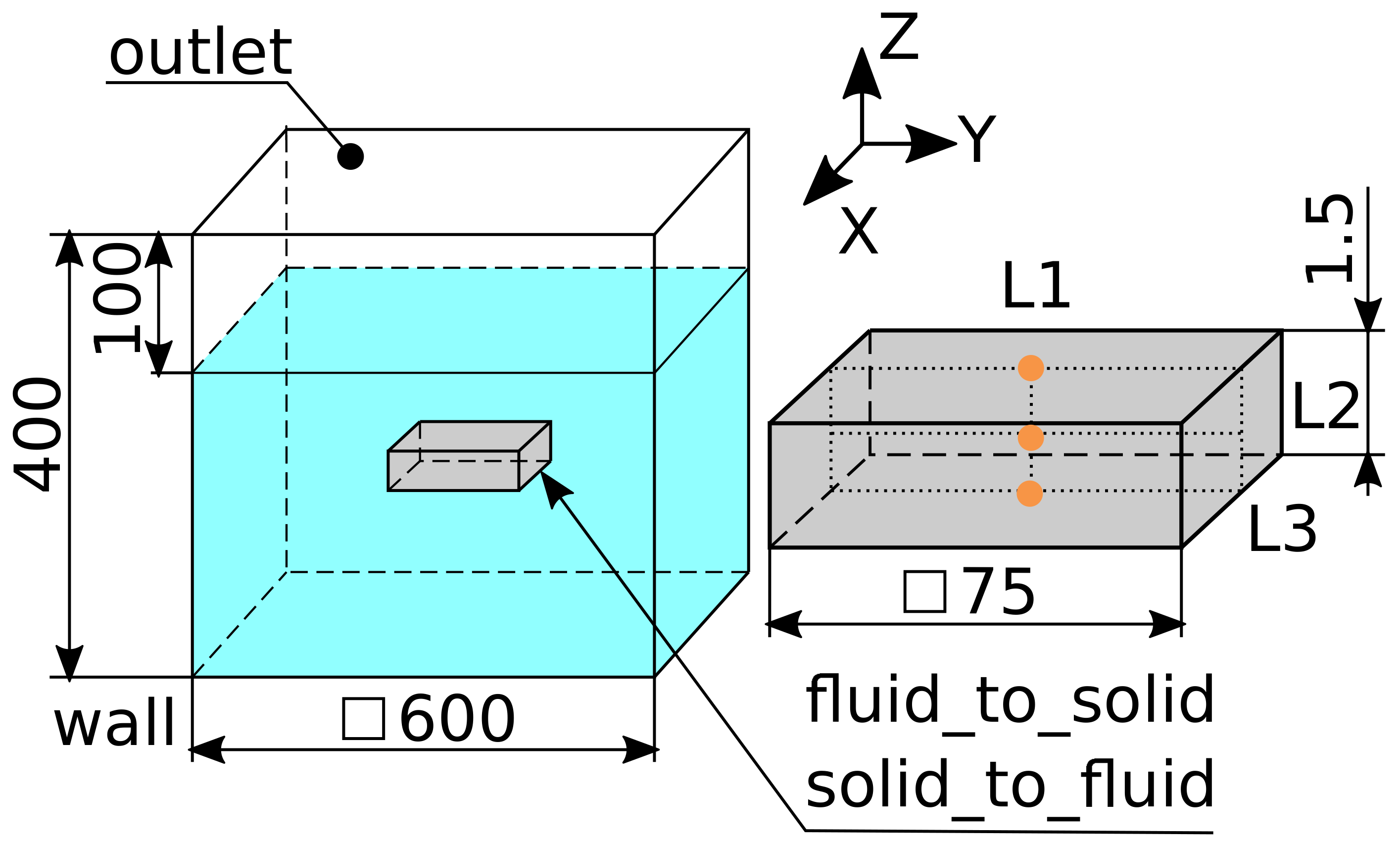
4.1. Geometry, Initial and Boundary Conditions

The computational domain consists of a tank filled with water up to three-quarters of its height (Figure 3). Vapour (air) fills the volume above the water surface, and both fluid phases are initially still. Agitation is not used, so fluid phase movements are driven only via density differences and their interactions. The heated sample is located in the centre of the tank. We do not account for the submerging effect. The water is at 25 °C, and the sample preheats to 880 °C. The physical properties of all three phases used for simulations follow Khalloufi et al. [18], meaning incompressible liquid and constant properties, except for the vapour density, which is subject to the ideal gas law instead of being a constant value (

Table 5. Physical properties of water, vapour and the plate specimen.

	$\mathit{\kappa }$ [W/(mK)]	${\mathit{c}}_{\mathit{p}}$ [J/(kgK)]	$\mathit{\rho }$ [kg/m${}^3$]	$\mathit{\mu }$ [Pa s]
solid	11.4	435	8000	-
liquid	0.6	4185	1000	0.001
vapour	0.025	2010	$\rho (p,T)$	0.000012

).

Figure 3 visualises all four boundary conditions and their names. The quenching tank bounding the computational domain represents a $wall$, and at the top is an $outlet$. The solid–fluid interface encloses the sample. That can either be the solid region $solid\_to\_fluid$ or the fluid region $fluid\_to\_solid$ boundary condition.

Table 6. Horizontal plate boundary conditions. ${\varphi }_{n,j}$ stands for mass flow rate through a boundary cell face.

	${\mathit{u}}_{\mathit{j}}\left[\frac{\mathit{m}}{\mathit{s}}\right]$	${\mathit{T}}_{\mathit{L}}$ [${}^{\circ }$C]	${\mathit{T}}_{\mathit{V}}$ [${}^{\circ }$C]	${\mathit{T}}_{\mathit{S}}$ [${}^{\circ }$C]
wall	noSlip	25	25	-
outlet ${\varphi }_{n,j}>0$	${\nabla }_{\widehat{\mathit{n}}}{\mathit{u}}_j=0$	${\nabla }_{\widehat{\mathit{n}}}{T}_L=0$	${\nabla }_{\widehat{\mathit{n}}}{T}_V=0$	-
outlet ${\varphi }_{n,j}\le 0$	$\frac{{\varphi }_j}{{\rho }_j{A}_B}\widehat{\mathit{n}}$	25	25	-
fluid_to_solid	noSlip	$T_V^I$	Section 3.2	-
solid_to_fluid	-	-	-	Section 3.2

defines some of the necessary variables boundary conditions. The temperature boundary conditions at both sides of the solid–fluid interface follow the description in Section 3.2. A simplification emerges assuming $T_L^I=T_V^I$, which allows estimating only one of the two and then setting the other at an equivalent value.

For the outlet patch, we can see that the velocity treatment depends on the flow direction. A zero gradient boundary condition is applied when the flow is positive, meaning the vapour/liquid leaves the domain. When we experience an inflow, the velocity boundary condition is calculated from the boundary condition face normal component of boundary cell mass flux. However, water cannot enter the domain as we set its volume fraction for inflow as zero. Only vapour (air) can enter. Finally, the description of the boundary condition for thermal turbulence diffusivity (wall boiling) at the solid–fluid interface matches the interpretation in Section 3.1.

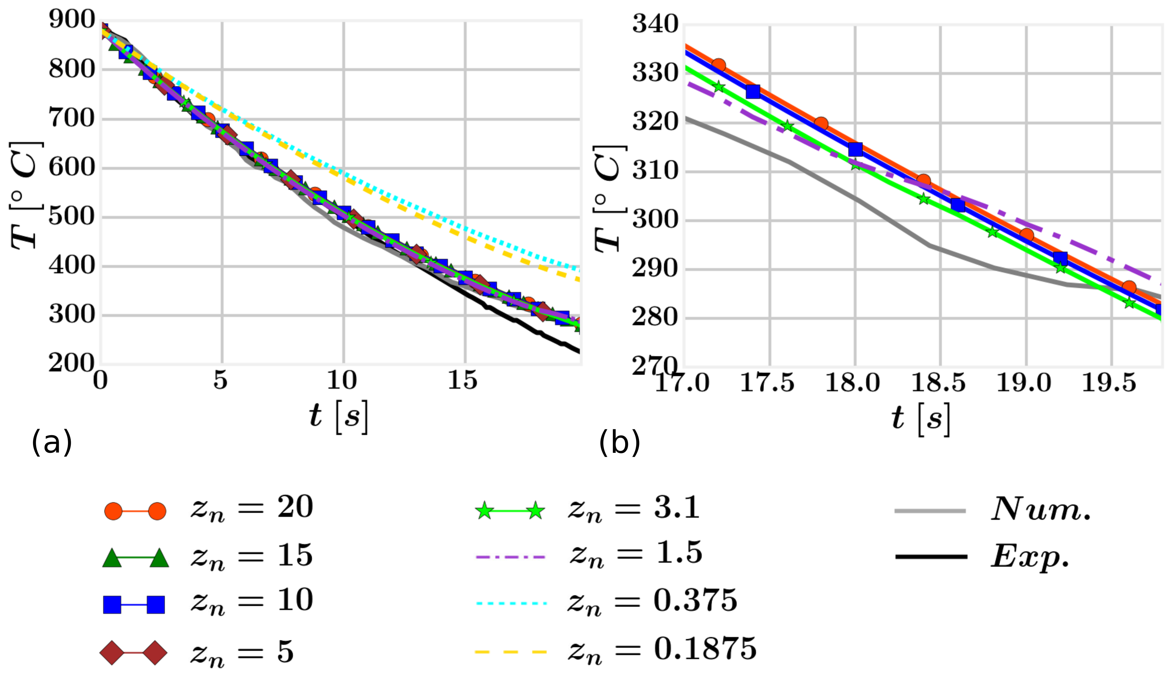
4.2. Mesh Definition

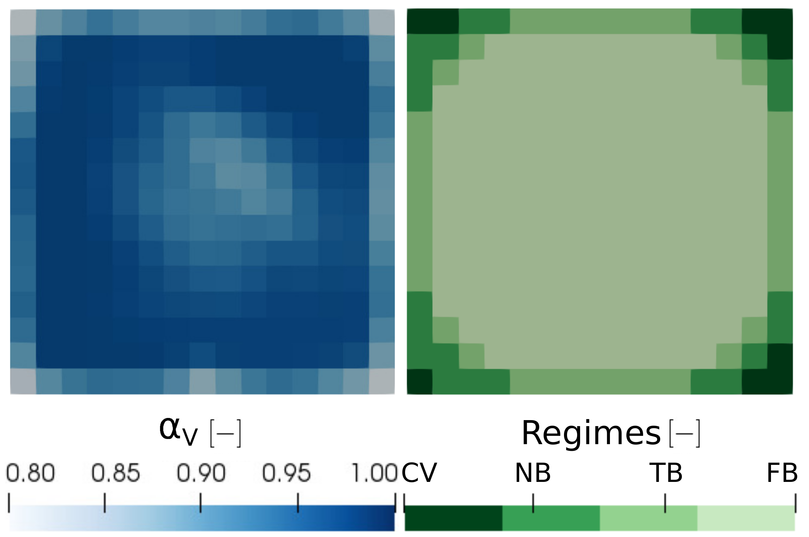
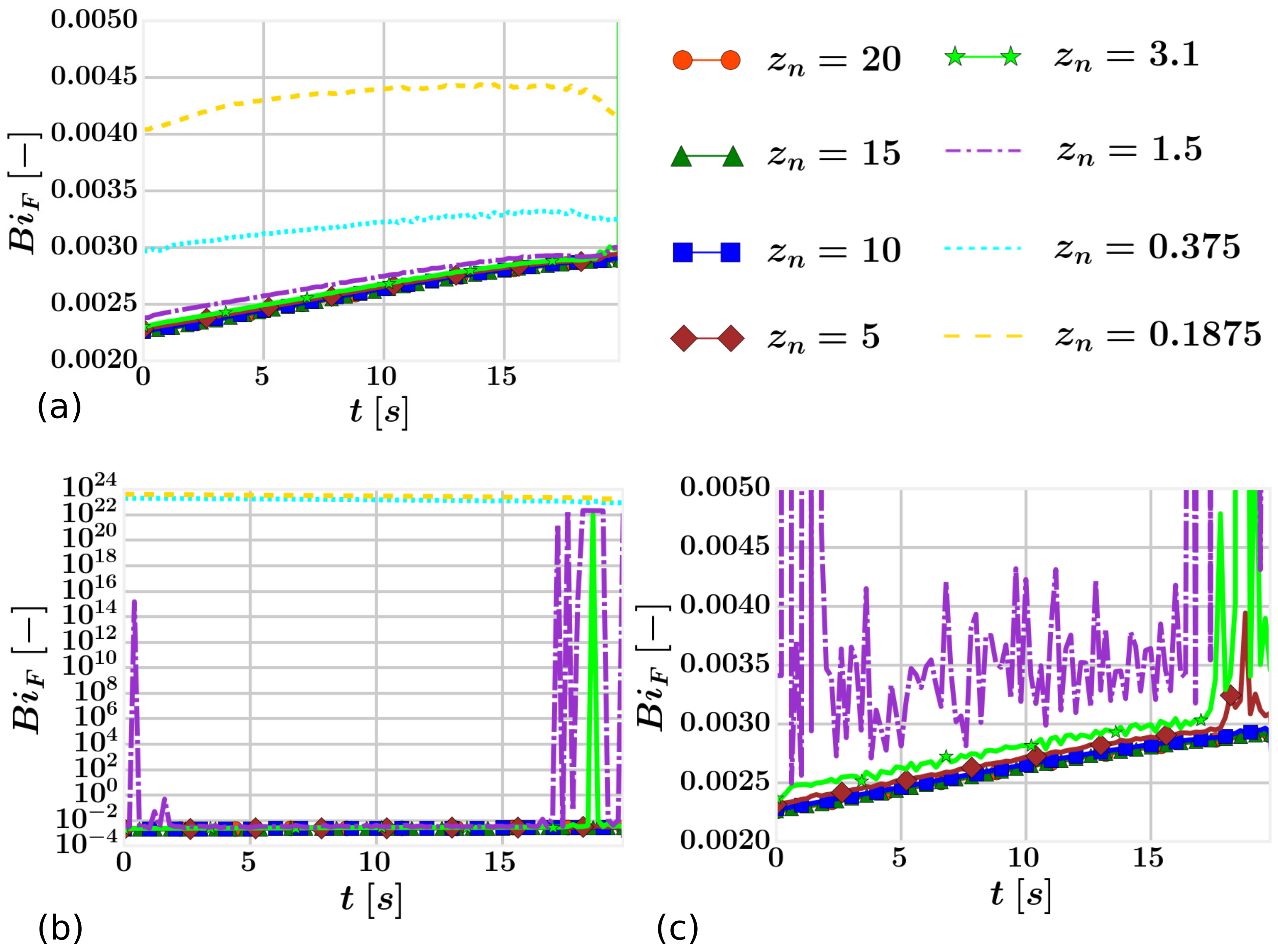
Before discussing the mesh and its behaviour, we would like to consider a few implications of the ETF method. Both fluid phases, vapour and liquid, can be viewed as dispersed and continuous phases. Nonetheless, the governing equations assume both phases to be continuous. Michaelides et al. [57] name this requirement for the dispersed phase the particle-phase continuum assumption. It follows that the particle (bubble/droplet) diameter must be smaller than the smallest dimension of the CoV the particle is present within, hence restricting the cell size:

$$D<\Delta x.$$

(39)

This requirement is also apparent, recalling the point force approach’s usage to account for the phase interaction. We do not resolve fluid disturbances due to individual particles. Instead, they are modelled and applied within each CoV. The apparent conclusion is that we have a limit arising from particle size and CoV size ratio. The limit places restrictions on resolving the computational domain’s geometrical features where the CoVs would have to be smaller than the presented particle. The matter, however, seems to be rarely discussed or followed in the literature [6,7,8,9,10,11,12,13,14,15,16,28]. The reason might be the limit’s forgiving behaviour. Violation of these restrictions does not necessarily lead to unphysical results. Numerical stability issues also might not occur unless the breach is significant. Moreover, considering an error stemming from the usage of the various interfacial correlations (models), the error due to the violation of this assumption can be negligible.

Comparing the bubble diameter of 3 mm with the plate thickness of 1.5 mm shows that the geometrical feature is smaller than the diameter. Nonetheless, it is essential to have at least one CoV across the plate thickness in the fluid region. We have not observed any adverse effects using this strategy.

We have decided on a purely hexahedral block-structured mesh with a locus on the plate’s horizontal surfaces. The mesh at the plate thickness is not that significant due to its negligible dimension compared to the other plate surfaces. During the study, we use several meshes with varying refinement labelled with the variable $z_n$ [mm], which represents the boundary cell size in the normal direction to the solid–fluid interface at the top and bottom plate surfaces. The goal is, alongside the methodology validation, to study the implication of this type of refinement due to its impact on the wall mass source terms via Equations (15), (19) and (24) and consequently on the whole computation. Results (Section 4.3) are displayed only for $z_n$ related to the fluid region. The solid region mesh refinement causes no significant behaviour anomaly and converges with four cells across the plate thickness. A summary of the mesh characteristics, including the total number of elements, refinement in each coordinate and boundary cell size, is given in

Table 7. Fluid and solid regions’ meshes characteristics, mentioning the total number of elements, the number of elements in x, y, z coordinates and boundary cells interface perpendicular dimension $z_n$ identical at the specimen top and bottom. Growth ratio within the fluid region is used. Its value is around 1.1, never exceeding it.

	No el.	No el. x-y-z	${\mathit{z}}_{\mathit{n}}$ [mm]
Fluid	27,950 40,842 57,094 123,800 219,475 278,625 367,350 422,275	35-35-23 39-39-27 43-43-31 55-55-41 65-65-52 65-65-66 65-65-87 65-65-100	20.0 15.0 10.0 5.0 3.1 1.5 0.375 0.1875
Solid	900	15-15-4	0.375

. The regions’ meshes are always conformal at the top and bottom surface to avoid interpolation errors.

4.3. Results

This section aims to validate the solver, indicate best practices for obtaining good quality results, and highlight any weaknesses, thus motivating further development. A wide range of data acquired at various locations, including those shown in Figure 3, are discussed. Our simulations always run for 19.8 s, which is the duration of the experiment used for validation [18]. In addition to the experiment, we compare the results to the numerical solution published in the same article [18]. We often use markers to distinguish curves in figures; however, these do not display all available data points.

We start by comparing the behaviour of various fluid meshes without IPC as assumed previously in the literature [6,7,8,9,10,11,12,13,14,15,16]. Figure 4a depicts cooling curves at the location $L2$ (Figure 3). The first observation reveals results converging for mesh configurations $z_n\ge$ 3.1 mm. These are also in excellent consensus with the numerical validation solution and good agreement with the experiment [18]. However, as the mesh is further refined, a considerably lower cooling rate emerges for meshes $z_n\le$ 0.375 mm. At the same time, $z_n$ = 0.1875 mm causes faster cooling than $z_n$ = 0.375 mm. When we focus on the mesh $z_n$ = 1.5 mm in a time range of 17–19.8 s (Figure 4b), we witness more moderate cooling at about 18.2 s, leading to a potentially significant shift of $T_{LEID}$ in time and misprediction of the cooling behaviour. Thus the mesh $z_n$ = 1.5 mm seems to be a limiting one between the converged refinements and the rest.

Investigation into the vapour volume fraction at $L1$ Figure 5a and $L3$ Figure 5b (the nearest locations to $L2$, where this data can be acquired) can provide us with some clues. We can see that, regardless of the location, the vapour volume fraction grows with the mesh refinement. The trend is even more visible at the bottom side of the plate, where vapour is more restricted from movement than at the top surface. While the vapour volume fraction reaches the maximum for meshes $z_n\le 0.375$ mm at $L3$, a considerable jump appears between the two and the other meshes at $L1$. That results from vapour isolation and heat diversion from the bottom to the top surface. Recalling the temperature results in Figure 4a, we observe that the cooling curves for meshes $z_n\ge 3.1$ mm do not change even though the volume fraction does. That can only be when the total heat flux from a particular location does not change. Indeed, meshes $z_n\le 1.5$ mm experience significant drops in the heat flux from the solid–fluid interface into the fluid at the location $L3$ and a substantial increase at location $L1$. Nevertheless, the increased heat transfer does not compensate for the reduction at the bottom plate surface, and the solid region temperature decrease becomes more moderate.

The steep increase in the vapour volume fraction, starting from about 17 s, appears due to the HTRs change. It has a limited effect on the measured cooling curve at $L2$, yet a crucial impact on the surroundings and influences the volume fraction at $L1$ and $L3$. It is also vital for the temperature gradient throughout the solid domain, but no experimental data are available.

The volume fraction is not necessarily mesh independent because the wall boiling mass source is applied within boundary cells only. That leads to increased vapour volume fraction with decreased boundary cell volume if the source term is constant. Nonetheless, the mass source is a function of volume fraction, making it also mesh dependent. Physically, we refine the vapour layer at the wall with increased refinement.

The vapour volume fraction and local HTRs at the plate bottom surface are depicted for mesh $z_n=3.1$ mm (see Figure 6) at 18.2 s. We can observe a wetting front where the film boiling faces are adjacent to transition and nucleate boiling HTRs. The phenomenon concentrates at corners and edges, thus locations that undergo the quickest cooling. We can also notice where the vapour is being developed and trapped. We already know that more vapour tends to be produced during the transition and nucleate boiling. Thus, vapour should be expected mainly along the wetting front.

Here we want to discuss why further mesh refinement, meshes $z_n\le 1.5$ mm, does not lead to mesh independent temperature results. We use the $B{i}_F$ Equation (38) plotted in Figure 7. The fluid Biot number considers all three phases interacting at the solid–fluid interface, taking into account their properties, volume fractions and regions’ meshes. We can observe meshes $z_n\ge 5$ mm to be converged at both locations $L1$ and $L3$. Only a little increase going hand in hand with refinement is notable. Significant jumps, however, appear for meshes $z_n\le 0.375$ mm at $L1$, and a severe problem emerges at the location $L3$. Looking at Equation (38), we deduce that this might happen when the solid temperature gradient is significantly greater than the fluid region temperature gradient. Meshes $z_n\le 0.375$ mm cause the vapour volume fraction at $L3$ to approach unity which prevents boiling. That leads to the liquid Biot number being equal to zero and so fluid temperature to be dictated solely by vapour temperature according to Equation (37). This would not be an issue unless the heat still flows into vapour at a high rate causing the temperature gradient between vapour and the solid–fluid interface to become marginal. An absent temperature gradient between a wall and the free stream for one-phase flow can lead to singularities in the heat transfer coefficient, as previously discussed by Schlichting and Gersten [58]. The non-converging behaviour observed previously in this section can be explained by a similar singularity that arises when the liquid in the near-wall cell boils completely, leading to an abrupt change of the thermal boundary layer.

Fluid temperature $T_F$, following Equation (37), in the boundary cell centre at the location $L3$, is visualised in Figure 8a. Indeed, it is apparent that the fluid temperature approaches the solid–fluid interface temperature for $z_n\le 0.375$ mm, occasionally for $z_n=1.5$ mm. Although the marginal temperature gradient also looms for $z_n=3.1$ mm, the impact can be disregarded because such conditions arise only for a very brief moment. $z_n\le 1.5$ mm retain these circumstances for a substantially more extended period. We also perceive that problems occur only once the fluid temperature exceeds saturation temperature.

In the second part of the methodology validation, we decided to examine the impact of IPC. Figure 9 is directly comparable with Figure 4, with the only difference being the IPC. We can state that meshes $z_n\ge 3.1$ mm behave equivalently. Even more, $z_n=1.5$ mm does not exhibit any severe anomaly. Nevertheless, meshes $z_n\le 0.375$ mm manifest considerable distinction. They reveal an effect of other HTRs due to more rapid cooling and reaching of the Leidenforst point quicker.

Examining the fluid Biot number $B{i}_F$ (Figure 10) and fluid temperature (Figure 8b), we observe, in comparison with the problem without IPC, a considerable improvement for $z_n=3.1$ mm and $z_n=1.5$ mm. Moreover, mesh configurations $z_n\le 0.375$ mm also no longer exhibit singular $B{i}_F$ values for prolonged periods. These are rather replaced by sporadic spikes accompanied by $T_F$ reaching the solid–fluid interface temperature. That being said, fluid Biot number no longer indicates a major issue yet might imply limiting configuration or probably numerical instability. The critical observation is fluid temperature fluctuation and mainly overstepping the saturation temperature, leading to interfacial boiling. That is not the case for meshes $z_n\ge 1.5$ mm, where interfacial condensation takes place exclusively.

Another profound distinction against the cases without IPC is the liquid–vapour interfacial temperature $T_f$ defined according to Equation (5). As discussed in Section 2.2.3, IPC assumes the interfacial temperature to be equal to the saturation temperature. In contrast, when the IPC is not activated, the liquid–vapour interfacial temperature can vary significantly. A maximum of the liquid–vapour interfacial temperature from boundary cells’ centres is visualised for both cases without IPC (Figure 11a) and with IPC (Figure 11b). The former shows a clear and substantial increase in temperature for $z_n\le 1.5$ mm compared to the rest of the meshes, which stay at lower magnitudes with minor fluctuation. Furthermore, similarly to the fluid temperature, the problematic meshes cause the liquid–vapour interfacial temperature to rise over $T_{SAT}$. The latter displays the enforced assumption of $T_f=T_{SAT}$. It starts to deviate once a change of HTRs takes place. It is not clear whether the transition complicates the compliance with the assumption. The above is a subject of future research.

To summarise, cooling curves, which are the most important for the problem in question, are acceptable for $z_n\ge 3.1$ mm without IPC and $z_n\ge 1.5$ mm with IPC. They also agree well with numerical validation data and are slightly lacking behind experimental results. The IPC usage improves the cooling curves of all meshes, but dominantly $z_n=1.5$ mm, which is otherwise not usable. Fluid Biot number and fluid temperature in boundary cell centres provide acceptable values for $z_n\ge 5$ mm without IPC and for all grids with IPC if we disregard occasional spikes, which might indicate numerical stability and accuracy issues. All problematic cases exhibit a fluid temperature above the saturation temperature and nonphysical fluid Biot numbers caused by an absence of fluid temperature gradient in the vicinity of the solid–fluid interface. Furthermore, when we enable IPC, configurations experiencing interfacial boiling exhibit distinct behaviour compared to those with only interfacial condensation. Our research has validated the solution methodology and has clearly shown that either fluid Biot number or fluid temperature in boundary cells should be monitored and used to evaluate computational results. For accuracy reasons and based on our analysis, we propose to avoid singular values of Biot fluid number.

5. Conclusions

We validated the computational fluid dynamics methodology developed for boiling conjugate heat transfer using the open-source toolbox OpenFOAM and described its key elements. In comparison with the previous research, substantial changes have been made, some of which are: consideration of additional heat transfer regimes, separate fluid phases energy equations, phase inversion, interfacial phase change and extra interfacial forces. Furthermore, we presented a detailed analysis of boiling conjugate heat transfer, which also applies to conjugate heat transfer into a two-phase fluid without boiling. That included the derivation of a temperature and Biot number governing fluid phases and impacting the solid–fluid interface. We then applied these two variables to describe the solver behaviour, assess computational results and develop guidance for a stable computational solution.

The validation focused on film boiling using an immersion quenching experiment with a high-temperature horizontal plate characterized by distinct heat transfer behaviour per surface. The bottom surface restricted vapour movement, while the top surface allowed the vapour to detach freely. Nevertheless, we also discussed the role of other heat transfer regimes and qualitatively assessed their behaviour.

We have shown that the results might be tedious to judge, as solid–fluid interface orthogonal refinement might alter them. Nonetheless, we found that these cases appear solely when an excessive fluid Biot number due to the marginal temperature gradient between the fluid and solid–fluid interface is determined. This phenomenon results from an abrupt change of the thermal boundary layer caused by the complete evaporation of liquid in the wall vicinity. Finally, the impact of interfacial phase change in addition to wall boiling was investigated. We found that it improves cooling curves results but can lead to distinct behaviour with fluid temperature fluctuation when interfacial boiling occurs.

Follow up research is in progress, focusing on applying the findings to more complex geometries and across the whole cooling curve temperature range. The influence of bubble dynamics is under consideration. Future research should also investigate the sensitivity of the methodology to various parameters, for example, subcooling and submerging effects. Although the proposed methodology is general enough so it can be applied to a wide range of problems, some models might need to be adapted accordingly.

References

1. Hernandez, R.; Folsom, C.P.; Woolstenhulme, N.E.; Jensen, C.B.; Bess, J.D.; Gorton, J.P.; Brown, N.R. Review of pool boiling critical heat flux (CHF) and heater rod design for CHF experiments in TREAT. Prog. Nucl. Energy 2020, 123, 103303. [Google Scholar] [CrossRef]
2. Kamenický, R.; Domalapally, P.K.; Arnoult, X. Thermo-mechanical stress analysis of the water cooled DEMO First Wall mock-up components. Fusion Eng. Des. 2018, 136, 1618–1623. [Google Scholar] [CrossRef]
3. Kalani, A.; Kandlikar, G.S. Enhanced Pool Boiling with Ethanol at Subatmospheric Pressures for Electronics Cooling. J. Heat Transf. 2013, 135, 111002. [Google Scholar] [CrossRef] [Green Version]
4. Liscic, B.; Tensi, H.; Canale, L.; Totten, G. Quenching Theory and Technology, 2nd ed.; CRC Press: Boca Raton, FL, USA, 2010. [Google Scholar]
5. Kulacki, F.A. (Ed.) Handbook of Thermal Science and Engineering; Springer: Cham, Switzerland, 2018. [Google Scholar]
6. Wang, D.M.; Alajbegovic, A.; Su, X.; Jan, J. Numerical modelling of Quench Cooling Using Eulerian Two-Fluid Method. In Proceedings of the ASME 2002 International Mechanical Engineering Congress and Exposition, New Orleans, LA, USA, 17–22 November 2002; pp. 179–185. [Google Scholar]
7. Wang, D.M.; Alajbegovic, A.; Su, X.; Jan, J. Numerical Simulation of Water Quenching Process of an Engine Cylinder Head. In Proceedings of the ASME/JSME 2003 4th Joint Fluids Summer Engineering Conference, Honolulu, HI, USA, 6–10 July 2003; pp. 1571–1578. [Google Scholar]
8. Srinivasan, V.; Moon, K.; Greif, D.; Wang, D.; Kim, M. Numerical simulation of immersion quench cooling process using an Eulerian multi-fluid approach. Appl. Therm. Eng. 2010, 30, 499–509. [Google Scholar] [CrossRef]
9. Srinivasan, V.; Moon, K.; Greif, D.; Wang, D.M.; Kim, M. Numerical simulation of immersion quenching process of an engine cylinder head. Appl. Math. Model. 2010, 34, 2111–2128. [Google Scholar] [CrossRef] [Green Version]
10. Greif, D.; Kovacic, Z.; Srinivasan, V.; Wang, D.M.; Suffa, M. Coupled Numerical Analysis of Quenching Process of Internal Combustion Engine Cylinder Head. BHM Berg- Hüttenmännische Mon. 2009, 154, 509. [Google Scholar] [CrossRef]
11. Jan, J.; Prabhu, E.; Lasecki, J.; Weiss, U.; Kaynar, A.; Eroglu, S. Development and Validation of CFD Methodology to Simulate Water Quenching Process. In Proceedings of the ASME Conference: International Manufacturing Science and Engineering Conference, Detroit, MI, USA, 9–13 June 2014. [Google Scholar]
12. Kopun, R.; Škerget, L.; Hriberšek, M.; Zhang, D.; Stauder, B.; Greif, D. Numerical simulation of immersion quenching process for cast aluminium part at different pool temperatures. Appl. Therm. Eng. 2014, 65, 74–84. [Google Scholar] [CrossRef]
13. Kopun, R.; Škerget, L.; Hriberšek, M.; Zhang, D.; Edelbauer, W. Numerical Investigations of Quenching Cooling Processes for Different Cast Aluminum Parts. Stroj. Vestn. 2014, 60, 571–580. [Google Scholar] [CrossRef] [Green Version]
14. Zhang, D.S.; Kopun, R.; Kosir, N.; Edelbauer, W. Advances in the numerical investigation of the immersion quenching process. IOP Conf. Ser. Mater. Sci. Eng. 2017, 164, 012004. [Google Scholar] [CrossRef] [Green Version]
15. Jan, J.; Mackenzie, D.S. On the Characterization of Heat Transfer Rate in Various Boiling Regimes Using Quenchometers and Its Application for Quenching Process Simulations. In Proceedings of the Thermal Processing in Motion 2018, Spartanburg, SC, USA, 5–7 June 2018; pp. 112–123. [Google Scholar]
16. Jan, J.; MacKenzie, D.S. On the Development of Parametrical Water Quenching Heat Transfer Model Using Cooling Curves by ASTM D6200 Quenchometer. J. Mater. Eng. Perform. 2020, 29, 3612–3625. [Google Scholar] [CrossRef]
17. Krause, F.; Schüttenberg, S.; Fritsching, U. Modelling and simulation of flow boiling heat transfer. Int. J. Numer. Methods Heat Fluid Flow 2010, 20, 312–331. [Google Scholar] [CrossRef]
18. Khalloufi, M.; Valette, R.; Hachem, E. Adaptive Eulerian framework for boiling and evaporation. J. Comput. Phys. 2019, 401, 109030. [Google Scholar] [CrossRef]
19. AVL FIRE. Available online: https://www.avl.com/fire (accessed on 8 February 2022).
20. Smith, M. ABAQUS/Standard User’s Manual, Version 6.9; Dassault Systèmes Simulia Corp: Johnston, RI, USA, 2009. [Google Scholar]
21. Verstraete, T.; Scholl, S. Stability analysis of partitioned methods for predicting conjugate heat transfer. Int. J. Heat Mass Transf. 2016, 101, 852–869. [Google Scholar] [CrossRef]
22. Weller, H.G.; Tabor, G.; Jasak, H.; Fureby, C. A tensorial approach to computational continuum mechanics using object-oriented techniques. Comput. Phys. 1998, 12, 620–631. [Google Scholar] [CrossRef]
23. Kurul, N.; Podowski, M. Multidimensional effects in forced convection subcooled boiling. In Proceedings of the Ninth International Heat Transfer Conference, Jerusalem, Israel, 19–24 August 1990; Volume 2, pp. 21–26. [Google Scholar]
24. Peltola, J.; Pättikangas, T.J.H. Development and validation of a boiling model for OpenFOAM multiphase solver. In Proceedings of the CFD4NRS-4 Conference Proceedings, Daejeon, Korea, 10–12 September 2012. [Google Scholar]
25. Jayatilleke, C.L.V. The Influence of Prandtl Number and Surface Roughness on the Resistance of the Laminar Sub-Layer to Momentum and Heat Transfer. Ph.D. Thesis, Imperial College of Science and Technology, London, UK, 1966. [Google Scholar]
26. Lahey, R.T. The simulation of multidimensional multiphase flows. Nucl. Eng. Des. 2005, 235, 1043–1060. [Google Scholar] [CrossRef]
27. Behzadi, A.; Issa, R.; Rusche, H. Modelling of dispersed bubble and droplet flow at high phase fractions. Chem. Eng. Sci. 2004, 59, 759–770. [Google Scholar] [CrossRef]
28. Yeoh, G.H. Computational Techniques for Multi-Phase Flows: Basics and Applications, 1st ed.; Butterworth-Heinemann: Oxford, UK, 2010. [Google Scholar]
29. Launder, B.E.; Spalding, D.B. The numerical computation of turbulent flows. Comput. Methods Appl. Mech. Eng. 1974, 3, 269–289. [Google Scholar] [CrossRef]
30. Weller, H.G. Derivation, Modelling and Solution of the Conditionally Averaged Two-Phase Flow Equations; Technical Report; OpenCFD Limited: Bracknell, UK, 2002. [Google Scholar]
31. Rusche, H. Computational Fluid Dynamics of Dispersed TwoPhase Flows at High Phase Fractions. Ph.D. Thesis, Imperial College London, London, UK, 2002. [Google Scholar]
32. Alali, A.; Schöffel, P.J.; Herb, J.; Macian, R. Numerical investigations on the coupling of the one-group interfacial area transport equation and subcooled boiling models for nuclear safety applications. Ann. Nucl. Energy 2018, 120, 155–168. [Google Scholar] [CrossRef]
33. Baglietto, E.; Demarly, E.; Kommajosyula, R.; Lubchenko, N.; Magolan, B.; Sugrue, R. A Second Generation Multiphase-CFD Framework Toward Predictive modelling of DNB. Nucl. Technol. 2019, 205, 1–22. [Google Scholar] [CrossRef]
34. Tu, J.; Yeoh, G. On numerical modelling of low-pressure subcooled boiling flows. Int. J. Heat Mass Transf. 2002, 45, 1197–1209. [Google Scholar] [CrossRef]
35. Mamoru, I.; Seungjin, K.; Joseph, K. Development of Interfacial Area Transport Equation. Nucl. Eng. Technol. 2005, 37, 525–536. [Google Scholar]
36. Ishii, M.; Zuber, N. Drag coefficient and relative velocity in bubbly, droplet or particulate flows. AIChE J. 1979, 25, 843–855. [Google Scholar] [CrossRef]
37. Tomiyama, A.; Tamai, H.; Zun, I.; Hosokawa, S. Transverse migration of single bubbles in simple shear flows. Chem. Eng. Sci. 2002, 57, 1849–1858. [Google Scholar] [CrossRef]
38. Antal, S.; Lahey, R.; Flaherty, J. Analysis of phase distribution in fully developed laminar bubbly two-phase flow. Int. J. Multiph. Flow 1991, 17, 635–652. [Google Scholar] [CrossRef]
39. Burns, A.; Frank, T.; Hamill, I.; Shi, J. The Favre Averaged Drag Model for Turbulent Dispersion in Eulerian Multi-Phase Flows. In Proceedings of the 5th International Conference on Multiphase Flow, ICMF’04, Yokohama, Japan, 30 May–4 June 2004; Volume 392, pp. 1–17. [Google Scholar]
40. Otromke, M. Implementation and Comparison of Correlations for interfacial Forces in a Gas-Liquid System within an Euler-Euler Framework Computational Fluid Dynamics of Dispersed Two-Phase Flows at High Phase Fractions. Ph.D. Thesis, Mannheim University of Applied Sciences, Mannheim, Germany, 2013. [Google Scholar]
41. Ranz, W.E.; Marshall, W.R. Evaporation from Drops, Parts I and IId. Chem. Eng. Prog. 1952, 48, 141–146. [Google Scholar]
42. Van der Vorst, H.A. Bi-CGSTAB: A Fast and Smoothly Converging Variant of Bi-CG for the Solution of Nonsymmetric Linear Systems. SIAM J. Sci. Stat. Comput. 1992, 13, 631–644. [Google Scholar] [CrossRef]
43. Barrett, R.; Berry, M.; Chan, T.F.; Demmel, J.; Donato, J.; Dongarra, J.; Eijkhout, V.; Pozo, R.; Romine, C.; der Vorst, H.V. Templates for the Solution of Linear Systems: Building Blocks for Iterative Methods, 2nd ed.; SIAM: Philadelphia, PA, USA, 1994. [Google Scholar]
44. Behrens, T. OpenFOAM’s Basic Solvers for Linear Systems of Equations Solvers, Preconditioners, Smoothers; Technical Report; Technical University of Denmark: Kgs. Lyngby, Denmark, 2002. [Google Scholar]
45. Márquez Damián, S. An Extended Mixture Model for the Simultaneous Treatment of Short and Long Scale Interfaces. Ph.D. Thesis, Universidad Nacional Del Litoral, Santa Fe, Argentina, 2013. [Google Scholar] [CrossRef]
46. van Leer, B. Towards the ultimate conservative difference scheme. II. Monotonicity and conservation combined in a second-order scheme. J. Comput. Phys. 1974, 14, 361–370. [Google Scholar] [CrossRef]
47. Končar, B.; Krepper, E.; Egorov, Y. CFD modelling of subcooled flow boiling for nuclear engineering applications. In Proceedings of the International Conference Nuclear Energy for New Europe 2005, Bled, Slovenia, 5–8 September 2005. [Google Scholar]
48. Schroeder-Richter, D.; Bartsch, G. Analytical calculation of DNB-superheating by a postulated thermo-mechanical effect of nucleate boiling. Int. J. Multiph. Flow 1994, 20, 1143–1167. [Google Scholar] [CrossRef]
49. Bromley, L.A. Heat Transfer in Stable Film Boiling; Technical Report; Lawrence Berkeley National Laboratory: Berkeley, CA, USA, 1949.
50. Zuber, N. On the Stability of Boiling Heat Transfer; Technical Report; United States Atomic Energy Commission: Washington, DC, USA, 1958.
51. Hua, T.; Xu, J. Quenching boiling in subcooled liquid nitrogen for solidification of aqueous materials. Mater. Sci. Eng. A 2000, 292, 169–172. [Google Scholar] [CrossRef]
52. Tolubinsky, V.I.; Kostanchuk, D.M. Vapour bubbles growth rate and heat transfer intensity at subcooled water boiling. In Proceedings of the International Heat Transfer Conference 4, Paris-Versailles, France, 31 August–5 September 1970. [Google Scholar]
53. Lemmert, M.; Chawla, J.M. Influence of flow velocity on surface boiling heat transfer coefficient. Heat Transf. Boil. 1977, 237, 111–116. [Google Scholar]
54. Egorov, Y.; Menter, F. Experimental Implementation of the RPI Wall Boiling Model in CFX-5.6; Technical Report; ANSYS Gmbh: Darmstadt, Germany, 2004. [Google Scholar]
55. Bowring, R.W. Physical Model, Based on Bubble Detachment, and Calculation of Steam Voidage in the Sub-Cooled Region of a Heated Channel; Technical Report; Institutt for Atomenergi: Kjeller, Norway, 1962. [Google Scholar]
56. Cole, R. A photographic study of pool boiling in the region of the critical heat flux. AIChE J. 1960, 6, 533–538. [Google Scholar] [CrossRef]
57. Michaelides, E.E.; Crowe, C.T.; Schwarzkopf, J.D. Multiphase Flow Handbook; CRC Press: Boca Raton, FL, USA, 2017. [Google Scholar]
58. Schlichting, H.; Gersten, K. Boundary-Layer Theory, 9th ed.; Springer: Berlin/Heidelberg, Germany, 2017. [Google Scholar]
Figure 1. A schematic indicating the conditions for the various HTRs. The vertical axis shows the heat flux across the solid–fluid interface, while the horizontal axis indicates the wall temperature. The various HTRs are labelled by capital letters: FB—Film boiling, TB—Transition boiling, NB—Nucleate boiling, CV—Convective heat transfer. The various subscripts have the following meanings: LEID—Leidenfrost, DNB—a departure from nucleate boiling, SAT—saturation, MHF—minimum heat flux, CHF—critical heat flux.
Energies 15 04258 g001
Figure 2. (a) Solid–fluid interface mesh view; (b) Partitioned heat transfer into liquid and vapour; (c) Heat transfer into fluid.
Energies 15 04258 g002
Figure 3. Computational domain with dimensions, boundary conditions names and investigated locations on the sample marked using orange dots. L1—Above the plate centre at the solid–fluid interface; L2—Plate centre; L3—Beneath the plate centre at the solid–fluid interface.
Energies 15 04258 g003
Figure 4. Cooling curves acquired at the location L 2 in the solid region using various fluid meshes. The interfacial phase change is not activated. (a) Global view with validation data; (b) Focused view to a time range 17–19.8 s omitting results for z n = 15 ; 5 ; 0.375 ; 0.1875 , and the experimental results.
Energies 15 04258 g004
Figure 5. Vapour volume fraction using various fluid meshes. The interfacial phase change is not activated. (a) Location L 1 ; (b) Location L 3 .
Energies 15 04258 g005
Figure 6. Vapour volume fraction and HTRs at the plate bottom for mesh z n = 3.1 mm at 18.2 s. The interfacial phase change is not activated. Regimes: CV—convective heat transfer, NB—nucleate boiling, TB—transition boiling, FB—film boiling.
Energies 15 04258 g006
Figure 7. Fluid Biot number according to Equation (38) using various fluid meshes. The interfacial phase change is not activated. (a) Location L 1 ; (b) Location L 3 ; (c) Location L 3 focused on z n 1.5 mm.
Energies 15 04258 g007
Figure 8. Fluid temperature in the boundary cell according to Equation (37) at the location L 3 using various fluid meshes. (a) IPC is not activated; (b) IPC is activated.
Energies 15 04258 g008
Figure 9. Cooling curves acquired at the location L 2 using various fluid meshes. The interfacial phase change is allowed and validation data are shown.
Energies 15 04258 g009
Figure 10. Fluid Biot number according to Equation (38) at location L 3 using various fluid meshes and with IPC activated. (a) Global view (b) Focused view on z n 1.5 mm.
Energies 15 04258 g010
Figure 11. Maximum of liquid–vapour interfacial temperature according to Equation (5) from boundary cells centres using various fluid meshes. (a) IPC is not activated; (b) IPC is activated.
Energies 15 04258 g011