Abstract
Enhancing energy efficiency is globally regarded as an effective way to reduce carbon emissions. In recent years, the energy efficiency of China has gradually improved; however, energy consumption and CO2 emissions are still increasing. To better understand the reasons for this, we evaluated the energy rebound effect (RE) of 30 provinces in China over the period 2001–2017 by employing stochastic frontier analysis (SFA) and the system generalized method of moments (system-GMM) approach, and explored the extent to which the RE affects CO2 emissions. Asymmetric and regional heterogeneity analyses were also conducted. The results indicate that the national average RE was 90.47% in the short run, and 78.17% in the long run, during the sample period. Most of the provinces experienced a partial RE, with a backfire effect occurring in some provinces such as Guangxi and Henan. The RE was associated with significant increases in CO2 emissions; specifically, a 1% increase in the short-run RE led to an increase in CO2 emissions of approximately 0.818%, and a 1% increase in the long-run RE resulted in an increase in CO2 emissions of approximately 0.695%. Moreover, significant regional differences existed in the impact of the RE on CO2 emissions; in regions with high emissions and a high RE, the CO2 reduction effect from the marginal decline in the RE was much more pronounced than that in other regions.
1. Introduction
In recent years, global warming has become a crucial issue worldwide [1,2]. As the main contributor to increasing temperatures, CO2 emissions, and their reduction, have become the primary focus. Governments hope to achieve the goals of energy conservation and emission reduction by implementing energy efficiency improvement policies. However, the existence of the rebound effect poses a potential challenge to the emission reduction targets. The rebound effect (RE) refers to the fact that the expected energy savings resulting from the improved energy efficiency may be offset to a certain degree due to the additional energy demand caused by the change in economic agents’ behavior [3,4,5]. A study by Fowlie et al. [6] highlighted that the actual energy savings resulting from the enhancement of energy efficiency are lower than the expected energy savings due to the existence of the RE, resulting in misalignment between energy policies and energy-saving goals. In view of the additional energy demand generated from the RE, special attention deserves to be paid to the environmental impacts (i.e., CO2 emissions) of the RE.
During the past two decades, the Chinese government has implemented a series of policies to improve energy efficiency to reduce energy consumption and CO2 emissions. As Figure 1 shows, China′s energy efficiency has gradually improved under these policies in recent years. However, contrary to our expectations, although China’s energy efficiency improved over this period, its overall energy consumption did not decline, but increased (see Figure 2). Specifically, China’s total energy consumption nearly tripled from 2001 to 2021, from 1555 million tons of coal equivalent (Mtce) in 2001 to 5240 Mtce in 2021 [7]. At the same time, CO2 emissions in China also increased over this period. From 2001 to 2019, total carbon emissions in China increased by nearly 3.7 times, from 3284 metric tons (Mt) in 2001 to 12,290 Mt in 2019 [8]. Figure 3 depicts the evolution trend in CO2 emissions in 30 provinces in China; it can be seen from Figure 3 that CO2 emissions gradually increased during the past decades.
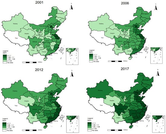
Figure 1.
Spatial distribution of energy efficiency performance in 30 provinces of China.
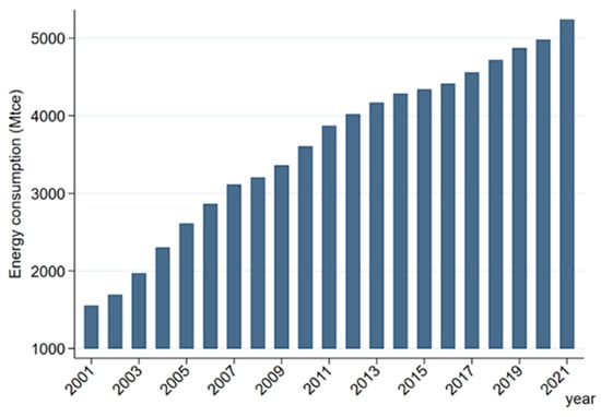
Figure 2.
Energy consumption in China, 2001–2021.
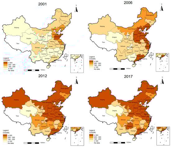
Figure 3.
CO2 emissions in China across 30 provinces.
The main driver behind this trend is the RE, which offsets potential energy savings from improved energy efficiency by generating new energy demand and thereby carbon emissions. However, the potential impact of the RE on CO2 emissions is often overlooked by energy policies. Since China is the world’s major CO2 emitter, it is worth paying attention to the impact of the RE on CO2 emissions, which would also provide valuable references for other countries with a high RE and high emissions.
In recent years, estimating the magnitude of the RE has become the focus of this research. Many scholars have evaluated the RE based on various approaches [9,10,11,12]; however, there is still a debate about its magnitude due to the lack of unified evaluation mechanisms both in theory and practice [13,14]. Furthermore, to date, much research has been undertaken to detect the potential drivers of CO2 emissions in terms of various aspects [15,16]; however, the potential impacts of RE on CO2 emissions have rarely been systematically investigated, especially for the case of China. To this end, several questions aroused our interest: (1) What is the extent of China′s current energy RE? Does the RE behave differently in the short and long term? (2) To what extent does the RE impact CO2 emissions in the short and long term? What is the direction of this impact? (3) Does the RE have asymmetric and heterogeneous regional impacts on CO2 emissions? It is essential to examine the above issues for a deeper understanding of the RE and its role in CO2 emissions, and thus provide new insights for policymakers to formulate emission reduction policies.
Accordingly, we first assessed the RE of 30 provinces in China from 2001 to 2017 by employing stochastic frontier analysis (SFA) and the system generalized method of moments (system-GMM) approach, and explored the extent to which the RE affects CO2 emissions. Asymmetric and regional heterogeneity analyses were also conducted. The contributions of this study are as follows: (1) By constructing a dynamic comprehensive energy efficiency index, we calculated the economy-wide RE of 30 provinces in China for the short and long terms. To the best of our knowledge, RE estimates are still lacking a consensus, and economy-wide RE studies at the sub-national level in China are rare. Considering the vast territory, resource endowment, and economic development differences in China, it is still necessary to investigate the RE at the sub-national level for a deeper understanding of the RE and to provide policymakers with new insights to formulate specific measures to control the RE. (2) To date, many studies have examined the potential drivers of CO2 emissions; however, very few studies have systematically explored the potential impacts of the RE on CO2 emissions, especially for the case of China. To make a marginal contribution to the existing literature based on this insight, we systematically explored the dynamic impacts of the RE in the short and long term on CO2 emissions based on the balanced panel dataset of 30 provinces in China, which offers strong evidence for capturing the potential drivers behind the continuous increase in CO2 emissions. This also provides valuable references for other countries with a high RE and high emissions, by offering policymakers new insights for designing short- and long-run policies from the perspective of the RE to reduce the carbon emissions. (3) Taking into account the regional heterogeneity, we also investigated the potential asymmetry and heterogeneity in the impact of the RE on CO2 emissions by dividing the full sample into four regions based on the distribution of the RE and CO2 emissions. This provides detailed evidence to design more specific regional policies to control the RE and CO2 emissions.
The remainder of the paper is organized as follows. Section 2 presents a brief literature review of the RE and determinants of CO2 emissions. Section 3 evaluates the RE of 30 provinces in China based on the stochastic frontier analysis (SFA) and system generalized method of moments (system-GMM) approach. In Section 4, we present an econometric model to explore the potential impacts of the RE on CO2 emissions; the data sources of all relevant variables are also reported in this section. Then, we discuss the impacts of the RE in the short and long run on CO2 emissions according to the econometric model estimation results in Section 5. In Section 6, we further conduct asymmetric and regional heterogeneity analysis of the impact of the RE on CO2 emissions. The final section presents the conclusions of this study.
2. Literature Review
2.1. Existing Research on the Energy Rebound Effect
In recent years, as a result of the increasing prominence of climate change, the energy rebound has attracted many scholars’ attention. The concept of the rebound effect dates back to Jevons [17]. In his book “Coal problem”, Jevons [17] noted that the increment in natural resource efficiency would result in increased consumption of such resources, rather than a decrease, which is known as the “Green paradox”. Subsequently, Daniel Khazzoom [18] and Brookes [19] initiated the modern rebound effect theory and debated the existence of a backfire effect in the real economy. Since then, many scholars have significantly explored the rebound effect.
In the literature, the measurement methods of the rebound effect are classified into two strands: computable general equilibrium (CGE) models and non-CGE models. In contrast to non-CGE models, CGE models are based on social accounting matrices for the relevant economies, and they consist of a set of simultaneous equations describing the behavior of producers, consumers, and other economic actors, together with the interdependencies and feedback between the different sectors [20]. Specifically, Bye et al. [9] calculated the energy rebound of Norway by employing a CGE model, and results indicate that Norway’s RE reaches 40% for the sample period. On the basis of a CGE model, Anson and Turner [21] investigated the RE of UK′s commercial transport sector. His study found that a 5% increase in energy efficiency in the commercial transportation sector resulted in a 39% rebound in the use of petroleum commodities in this industry and the whole economy. Based on the same method, Hanley et al. [22] explored the RE of Scotland’s economy and identified a backfire effect in Scotland’s power and non-power sectors, with rebounds of 131% and 134%, respectively. However, the CGE approach has been criticized by some scholars due to its strict assumptions, such as constant substitution elasticity between different input factors and complete market clearing [20], and it poses high requirements for data quality [23]. Therefore, some scholars also explored non-CGE models to estimate the RE, such as macroeconomic models, econometric analysis, and the growth accounting approach. Specifically, based on the macroeconomic model, i.e., the Solow growth model, Saunders [10] estimated Sweden’s energy RE for a long period between 1850 and 2000, and found that the average rebound value was approximately 60%. On the same basis, Barker et al. [24] explored the global RE for the period of 2010–2030 and indicated that the average value of the energy RE was 52%. With regard to econometric analysis, Adetutu et al. [11] explored the RE of 55 countries by employing stochastic frontier analysis and found that the RE reaches 90% in the short term, and −36% in the long term. Wei et al. [12] estimated the RE of 40 regions for the period 1995–2009 by decomposing the change in output caused by energy intensity variation, and found that the average RE is 150%. Some scholars also tried to evaluate the RE based on the growth accounting approach. For instance, Lin and Liu [25] estimated China’s RE between 1981 and 2009 by employing the growth accounting approach, and indicated that the average value of the RE was 53.2%. By utilizing the same technique, Shao et al. [14] evaluated China’s RE for the period 1954–2010 and found that the average value was 47% before 2000, and 37% after 2000. In summary, compared to the complex CGE model, studies based on non-CGE models have also contributed valuable insights; however, they also present a number of significant limitations. For instance, Saunders [10] and Wei et al. [12] adopted aggregate production functions, which were not believed to be appropriate by some scholars [26,27]. The growth accounting studies underestimated rebound effects, owing to their assumption that increases in output are the primary driver of rebound, which neglects other mechanisms of RE [5,28]. Overall, a large amount of work has been conducted to examine the rebound effect by developing different approaches; however, estimation results are still not consistent due to the lack of unified evaluation mechanisms, both in theory and practice [20,29].
As China has become the world’s major energy consumer, China’s energy rebound has also attracted many scholars’ attention. The related literature has mainly concentrated on exploring the RE (direct or indirect) of different industries, regions, or sectors (e.g., households). Specifically, Lin and Zhu [4] evaluated the direct RE of Chinese residents’ electricity consumption for the period 2010–2018, and the results indicate that the average RE was 48%. Based on the time series data of 1991–2016, Shao et al. [30] explored the RE of Shanghai, China, and found the total RE during this period reached 93.96%. Liu et al. [31] evaluated the RE of the coal industry in China from 2009 to 2019, and the results indicate that the average RE of the industry was 30.27%. Meng and Li [32] estimated the direct RE of the electricity sector in 30 Chinese provinces for the period 2009–2018, and found that the average RE was 75.21%. On the basis of a panel dataset over the period 2003–2013, Zhang and Lin [33] calculated the RE of the transport sector in China, and showed the extent of the RE varied from 7.2% to 82.2%. In addition, Du et al. [34] estimated the RE level of the Chinese urban residential sector for the period 2001–2014, and the results indicate that the average RE was 65.4%. Li and Lin [35] conducted a comparative study of the RE of light and heavy industries in China, and found the average RE of heavy industry was larger than that of light industry. In contrast to the above studies, a few scholars have also made efforts to investigate the economy-wide RE of China. For instance, Shao et al. [14] explored the economy-wide RE of China based on the time series data of 1954–2010, and the results indicated that the national average RE was 47.24% before 1978, and 37.32% after 1978. Zhang and Lin Lawell [36] calculated the macroeconomic RE of China during the period of 1991–2009, and found that the national average RE was −0.1421. Notably, studies of the economy-wide RE of China are relatively rare and the sizes of the RE are still not consistent. Considering the vast territory, resource endowment, and economic development differences in China, it is still necessary to investigate the economy-wide RE at the sub-national level for a deeper understanding of the RE. This will be helpful for providing policymakers with new insights to formulate specific measures to control the regional RE.
2.2. Research on the Determinants of CO2 Emissions
As a result of global warming, carbon reduction has become the primary task to deal with climate change. Many scholars have explored the drivers of CO2 emissions in terms of different aspects, such as economic growth, energy structure, urbanization, and trade openness. More specifically, the economic growth–CO2 nexus, which is known as the environmental Kuznets curve (EKC), has been examined extensively in the existing research. For example, by employing the ARDL approach on a panel dataset from 1971 to 2011, Shahbaz et al. [37] investigated the EKC hypothesis for Malaysia and found that there is significant inverted-“U”-type relationship between economic growth and CO2 emissions. This relationship was also confirmed by Esteve and Tamarit [38], Farhani et al. [16], Haisheng et al. [39], Iwata et al. [40], and Plassmann and Khanna [41]. Contrarily, some studies found little evidence supporting the EKC hypothesis. For instance, Zilio and Recalde [42] investigated the EKC hypothesis for the case of Latin America and the Caribbean for the period of 1970–2007, and found no support for this hypothesis. Based on the Engle–Granger test, Day and Grafton [43] also found little evidence for the validity of the EKC hypothesis for Canada. Notably, the nexus between economic growth and carbon CO2 emissions is still controversial. Moreover, studies have emphasized the important role of the energy structure on CO2 emissions. Specifically, by analyzing China’s energy consumption structure over the period 1980–2006, Feng et al. [44] suggested that reducing the proportion of fossil energy in total energy consumption and transforming to clean energy can effectively mitigate carbon emissions. This conclusion was confirmed by Xu et al. [45] and Wang et al. [46].
Furthermore, a significant amount of work has been undertaken to examine the relationship between urbanization and CO2 emissions, since the development of the urban economy requires sufficient energy input. Empirical results vary between studies, which have presented various views on the urbanization–CO2 emissions nexus. For instance, using a sample of developing countries over the period 1975–2003, Martínez-Zarzoso and Maruotti [47] examined the relationship between urbanization and CO2 emissions, and the research results indicate that there is an inverted-U-shaped relationship between urbanization and CO2 emissions. Contrarily, Shahbaz et al. [48] identified a significant U-shaped urbanization–CO2 emissions nexus for the case of Malaysia over the period of 1970–2011. In addition, Fan et al. [49] found a negative relationship between urbanization and CO2 emissions for the sample of developing countries, and Liddle and Lung [50] found a positive insignificant relationship between urbanization and CO2 emissions for the developed countries. In summary, the results regarding the relationship between urbanization and CO2 emissions have not been conclusive. In addition, scholars also examined the relationship between trade openness and CO2 emissions. Specifically, Mutascu [51] noted a one-way direction of causality from trade openness to carbon emissions in France over the period 1960–2013. Conversely, Shahbaz et al. [15] identified one-way causality running from CO2 emissions to trade openness in China over the period 1970–2012. Furthermore, some studies have also detected two-way causality [52,53]. Notably, the trade openness–CO2 nexus is still controversial within the literature. Furthermore, scholars also examined other influencing factors of CO2 emissions. For example, the research results of Wójcik-Jurkiewicz et al. [54] and Drożdż et al. [55] identified significant roles of knowledge diffusion and public perception on decarbonization in Poland. In conclusion, to date, many studies have explored the drivers of CO2 emissions in terms of various aspects; however, very few studies have systematically examined the potential impacts of the RE on CO2 emissions, especially for the case of China. In the context of a low-carbon economy, it is necessary to systematically explore the extent to which the RE influences CO2 emissions.
3. Materials and Methods
3.1. Measurement Procedure for Rebound Effect
As defined by Saunders [56], the rebound effect is:
where (E is the energy consumption, DEPI denotes energy efficiency), which represents the elasticity of energy consumption to the energy efficiency. We can obtain the RE by estimating .
We assumed that the optimal energy consumption of an enterprise is influenced by its output level, energy price, and energy efficiency. Following the work of Yan et al. [23] and Adetutu et al. [11], we constructed an optimal energy consumption function as follows:
where represents optimal energy consumption, and , , and represent energy prices, real GDP, and energy efficiency, respectively. and are the constant term and the disturbance term, respectively.
For a given improvement in energy efficiency, enterprises require a certain amount of time to adjust their energy use. Therefore, we also considered the actual energy consumption in the process of dynamic adjustment:
where represents the actual energy consumption, and is the adjustment proportion. Combining Equations (2) and (3), we obtained:
where , . By performing the second-order Taylor expansion on , we obtained:
According to the estimation parameters of Equation (5), we calculated the short- and long-run efficiency elasticity as follows:
Therefore, the RE in the short and long run can be obtained according to Equations (6) and (7):
Notably, we selected the price index of fuels (P2000 = 100) as the proxy for the energy price due to the absence of energy price data; this was derived from the CSY (2018) [57]. The data on energy efficiency were obtained from the calculation results in Section 3.2. The data on energy consumption were taken from the CESY (2018) [58], and the GDP data originated from the CSY (2018) [57], and are deflated based on the 2000 constant price.
3.2. Measurement Procedure for Energy Efficiency
To estimate efficiency elasticity (), we first need to measure the energy efficiency level. To this end, we constructed a dynamic comprehensive energy efficiency indicator (DEPI) that fully considers various input factors and changes in energy technology progress. To calculate the DEPI, we first needed to evaluate the Shephard energy distance function, which identifies the extent to which energy input factors decrease when other input factors remain the same in the production possibility set. We assumed that each decision-making unit, i.e., each province of China (), yields the desired output GDP (Y) based on the three inputs: capital (K), energy (E), and labor (L); where K is determined based on the perpetual inventory method using 2000 constant prices. E is determined using the provincial aggregate energy consumption. Each province′s employee count at the end of the year represents L, and Y is measured by real GDP using 2000 constant prices. All data were derived from China’s various statistical yearbooks. Following the work of Boyd and Pang [59] and Wu et al. [60], the Shephard energy distance function is expressed as:
where is an unknown function, represents an unobserved individual effect, and represents a random disturbance term. Using its second-order Taylor expansion, we approximated Equation (10) as follows:
Due to the linear homogeneity of the Shephard energy distance function with respect to energy factor inputs, the following relationship exists:
By combining Equations (11) and (12), we obtained:
where represents the inefficiency of energy use, which follows . Considering the stochastic frontier analysis (SFA) has obvious advantages in dealing with statistical noise and the heterogeneity of the reaction technology, we adopted the SFA method to estimate Equation (13). According to the parameter estimation results of Equation (13), we can estimate the static energy efficiency of each using the following equation:
where . Thus, the static energy efficiency change is calculated by the following equation:
Then, the change in energy technology progress is obtained by calculating the following equation:
Finally, the product of and is the dynamic comprehensive energy efficiency (DEPI), which is presented in Figure 1.
3.3. Econometric Model
After evaluating the RE, we empirically explored the potential impacts of the RE in the short and long term on CO2 emissions, and determined the validity of the CO2–EKC (environmental Kuznets curve) hypothesis. To avoid false regression problems, we considered the following control variables: economic development level, energy structure, urbanization, and trade openness. Thus, we constructed the CO2–EKC model as follows:
where CO2 represents the CO2 emissions of each province. SRE and LRE represent the short-run and long-run RE, respectively. Pgdp represents the economic development level, and Tra represents trade openness. ENS and Urb represent the energy structure and urbanization, respectively. are the parameters to be estimated by the model. is the constant term, and represents the random disturbance term.
3.4. Variable Selection and Data Sources
A panel dataset of 30 provinces in China, from 2001 to 2017, was used in this study for empirical analysis. The sample excluded Tibet, Taiwan, Hong Kong, and Macao because of data unavailability. The data on CO2 emissions were taken from the China Emission Accounts and Database [8]. The RE data for the key explanatory variables (represented by SRE and LRE, respectively), in the short and long run, were derived from the calculation results in Section 4.1.
Regarding the control variables, economic development (Pgdp) was measured by GDP per capita, energy structure (ENS) was measured by coal consumption as a percentage of total energy consumption, urbanization (Urb) was calculated by the ratio of permanent urban population to total population, and trade openness (Tra) was presented as the ratio of net trade imports and exports to aggregate GDP. All data were derived from various statistical yearbooks of China, which are reported in Table A1 in Appendix A. Detailed descriptive statistics are provided in Table 1 for all of the above variables.

Table 1.
Descriptive statistics of each variable.
4. Results
4.1. Rebound Effect Estimation Results
We used the system generalized method of moments (SYS-GMM) to evaluate the parameters in Equation (5), considering the dynamic feature of this model. The results are reported in Table 2. To ensure the estimation results were robust, the differential generalized method of moments (D-GMM) estimation results are also reported. The AR test showed no second-order autocorrelation existed, as shown in Table 1. Based on the Sargan test results, all instrumental variables selected by the model satisfied the exogenous conditions, which implies the validity of all instrumental variables. Moreover, compared to the D-GMM method, the estimation results of the SYS-GMM approach were significantly improved, which supports the appropriateness of utilizing the SYS-GMM method for this model.
Table 2.
Parameter estimation results.
Based on the parameter estimation results in Table 1, the RE value of each province was calculated in the short and long term. Figure 4 presents the average value of the RE in each province from 2001 to 2017. As clearly shown in Figure 4, most of the provinces experienced a partial RE during this period, but some provinces, such as Guangxi and Henan, experienced a backfire effect. The average RE across the nation was 90.47% in the short term, and 78.17% in the long term.
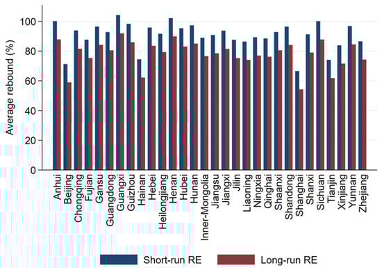
Figure 4.
Average RE of 30 Chinese provinces in the short and long run.
To clearly identify the evolution track of China′s RE, we drew spatial distribution maps of China’s RE, both in the short and long run, for 2001, 2006, 2012, and 2017, which are presented in Figure 5. Notably, two interesting phenomena attracted our attention from Figure 5. First, the RE was greater in the short run than in the long run. This may be because, in the context of low energy prices and marketization in China, energy prices have not adjusted in the short term to reflect the improvements in energy efficiency.
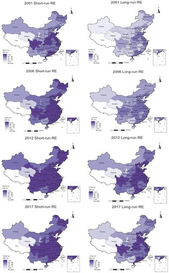
Figure 5.
Spatial distribution of China’s short-run and long-run RE.
Therefore, improving energy efficiency will greatly stimulate energy demand to a large extent in the short term, which leads to a steep discount of the potential energy savings from improved energy efficiency. In the long run, energy prices may adjust to some extent; in addition, knowledge accumulation and increased awareness of environmental conservation among economic agents, and environmental regulation policies, will encourage end-users to make more efficient use of energy. As a result, the energy-saving benefits of improved energy efficiency will be gradually realized in the long run.
Second, Figure 5 shows that most of the high-RE provinces are located in the central and eastern regions of the country. According to Orea et al. [61], energy prices and income levels are the main factors affecting the energy rebound. Because energy prices are relatively low and market oriented in China, this finding can be discussed further with consideration of regional economic development differences. Eastern China is a developed region having the highest GDP per capita (CNY 20,660.34 billion), whereas that of the central region is moderate (CNY 11,739.36 billion GDP per capita) and the western region is relatively poor (CNY 6952.39 billion GDP per capita) [62]. In light of the fact that rapid industrialization and urbanization are taking place in China at present, there are still no signs of a decoupling between regional economic growth and energy consumption. Due to the high income levels and large economic scale in the eastern and central regions, their energy consumption demand is far greater than that in the poorer western regions. Therefore, the rapid improvement in energy efficiency in these regions (as shown in Figure 1) stimulates significant energy demand. In the sample period, the average energy consumption in the eastern and central regions reached 139.96 and 109.94 Mtce, respectively, whereas that of the western region was only 68.88 Mtce [7]. Correspondingly, as shown in Figure 1, energy efficiency improvements in the western region are not obvious, and energy efficiency even deteriorated in some provinces. Therefore, the RE in the western region is not obvious due to the low energy efficiency and poor income level.
4.2. Econometric Model Estimation Results
4.2.1. Cross-Sectional Dependence Test Results
Grossman and Krueger [63] noted that ignoring cross-sectional dependence within panel data will affect the credibility of the estimation results, which may result in inconsistent evaluation results. Therefore, it is essential to perform a cross-sectional dependence test before empirical analysis is conducted [64]. For this purpose, we employed the Pesaran cross-sectional dependence test [65], Breusch–Pagan Lagrange multiplier test [66], Friedman test [67], and Frees test [68] to identify whether cross-sectional dependence exists. Table 3 reports the test results, and shows that, at the 1% significance level, all four tests rejected the null hypothesis of no cross-sectional dependence. Therefore, it was necessary to take into account cross-sectional dependence when performing the empirical analysis in this study.
Table 3.
Results of the cross-sectional dependence test.
4.2.2. Panel Unit Root Test Results
A stationarity check is necessary for each variable before empirical analysis is conducted to avoid invalid regression problems. We utilized the CIPS tests and Pesaran CADF test [69], which permit the existence of cross-sectional dependence [70], to detect stationarity for each variable in this study. Table 4 reports the results of the above two tests, and shows that only some variables (e.g., CO2, ENS, and Pgdp) are significant at the tested level. Therefore, we took the first-order difference for each variable. After taking the first-order difference, each variable rejected the null hypothesis (existence of a unit root) at the 1% significance level. Thus, each variable should be transformed into a variable having an order of one in the subsequent estimation procedure.
Table 4.
Panel unit root test results.
4.2.3. Benchmark Regression
We first drew the correlation plot between the RE and CO2 emissions, as presented in Figure 6, which shows that the RE measures (lnSRE and lnLRE) are positively correlated with CO2 emissions. Their goodness of fit values (R2), however, are only 0.2789 and 0.2854, respectively. Therefore, more accurate and efficient methods are needed in a further step to fully understand the impact of the RE on CO2 emissions.
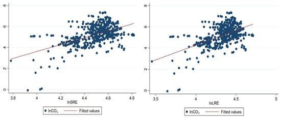
Figure 6.
Correlation diagram between RE and CO2 emissions.
The GMM method is more suitable for dynamic panel models (Equations (17) and (18)) considering their dynamic features, because it can solve the endogeneity problem by introducing reasonable instruments, thus effectively improving estimation results [71]. Specifically, the system GMM (SYS-GMM) approach can be used to introduce more effective instrumental variables, and to simultaneously estimate the level and difference equations, which improves the validity of estimation results compared with the difference GMM (D-GMM) method [72]. Therefore, we adopted the SYS-GMM estimation method as a benchmark and report the D-GMM estimation results due to their robustness. Table 5 presents the results; the AR test results indicate that second-order autocorrelation does not exist. All of the instrumental variables used in the model meet the exogenous conditions based on the results of the Sargan test, and thus are valid.
Table 5.
Results of modeling the impact of RE on CO2 emissions.
As can be seen in Table 5, both the short-run and long-run RE have significant positive impacts on CO2 emissions in China. Specifically, a 1% increase in the short-run RE leads to an increase in CO2 emissions of 0.818%, whereas a 1% increase in the long-run RE causes CO2 emissions to rise by approximately 0.695%. These results warrant great concern. The increasingly significant RE poses a potential challenge to the carbon reduction goals. To strengthen environmental protection and reduce greenhouse gas emissions, the central government of China proposed a “double control policy” in October 2015, which specifically aimed to control the total energy consumption and energy intensity. Improving energy efficiency is the key to reducing energy intensity and, subsequently, reducing total energy consumption. Driven by the strong national energy policy, China′s energy efficiency has gradually improved, as shown in Figure 1. However, the results of this study imply that the existence of a large RE is a potential challenge to achieving the energy-saving objectives outlined in the policies by solely relying on improved energy efficiency. Due to China′s vast territory, large population, and unbalanced regional development, many provinces are still at a stage of rapid industrialization and urbanization, which requires enormous energy input. Therefore, the rapid improvement in energy efficiency greatly stimulates energy consumption in the context of low energy prices and marketization in China, which results in more CO2 emissions.
Regarding the control variables, there is a significant positive effect of the energy structure on CO2 emissions, which indicates the urgency of the energy structure adjustment. The coefficient of per capita income is positive, but its quadratic term is negative; this implies the existence of an inverted-U-shaped nexus between per capita income and CO2 emissions, which proves the validity of the CO2–EKC hypothesis. Saboori et al. [73] and Dong et al. [74] also came to the same conclusions. In addition, urbanization presents a significantly positive effect on CO2 emissions. In light of China’s rapid urbanization, many rural laborers are migrating to cities, which creates demand for services such as housing and medical services. These additional demands inevitably propel energy consumption, and thus promote CO2 emissions. Finally, a positive estimate of trade openness implies that trade openness positively impacts China′s CO2 emissions. The possible reason for this is that increasing domestic and international trade may result in increased CO2 emissions due to the flow of factors between regions [75].
4.2.4. Robustness Checks
We performed a robustness test by introducing a new dependent variable, per capita CO2 emissions (denoted as PCO2), to determine the validity and reliability of the benchmark regression results. The test results from the SYS-GMM and D-GMM approaches are presented in Table 6. A comparison of the estimation results in Table 5 and Table 6 indicates that the core explanatory variables, e.g., short-run RE (lnSRE) and long-run RE (lnLRE), in addition to the other control variables, exhibit consistency, both in terms of coefficient size and statistical significance. This indicates the reliability and credibility of the benchmark regression results presented in Section 4.2.3.
Table 6.
Robustness test results using an alternative variable.
5. Discussion
5.1. Regional Heterogeneity Analysis
The distribution map of the RE and CO2 emissions exhibits obvious regional heterogeneity among different regions in China, as displayed in Figure 1 and Figure 3. Therefore, to understand whether the impacts of the RE on CO2 emissions differ across various regions, we grouped the whole sample based on the average value of the RE and the CO2 emissions of each province. Considering that the spatial distributions of short-run and long-run RE exhibit similar characteristics (as shown in Figure 5), the mean value of the two RE measures was utilized to represent the total RE for the groups. Therefore, the full sample was categorized into four groups: (1) the high-RE region, which includes the provinces having an RE greater than the national average; (2) the low-RE region, which includes the provinces having an RE lower than the national average; (3) the high-emission region, which includes the provinces having CO2 emissions higher than the national average; (4) and the low-emission region, which includes the provinces having CO2 emissions lower than the national average. The specific provinces in each group are presented in Figure 7.
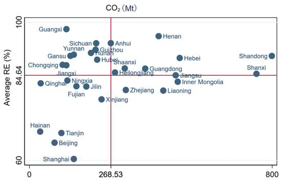
Figure 7.
Group division based on the RE and CO2 emissions of China’s 30 provinces.
Accordingly, on the basis of the SYS-GMM method, we explored the impacts of the RE on CO2 emissions across the four regions, and the results are reported in Table 7. It can be seen from this table that there are significant regional differences in the impact of the RE on CO2 emissions. In further detail, the RE positively affects CO2 emissions in both the high-emission and low-emission regions at the 1% significance level. Specifically, a 1% increase in the RE will lead to increases in CO2 emissions of approximately 0.655% in the high-emission region and 0.332% in the low-emission region. Notably, this positive impact in the high-emission region is greater than that in the low-emission region. A possible reason for this may be that, in high-emission regions, provinces such as Shanxi and Shandong are dominated by large-scale heavy industry, and urbanization is rapidly developing, both of which require great amounts of energy. Therefore, improved energy efficiency (as shown in Figure 1) increased energy consumption in these areas, resulting in a large RE (as shown in Figure 4), which caused an increase in CO2 emissions. In summary, reducing the RE will be conducive to mitigating CO2 emissions in both high-emission regions and low-emission regions in China. Furthermore, there is more scope for emissions reductions from the perspective of the energy rebound, especially for high-emission regions.
Table 7.
Results of the regional heterogeneity analysis.
In addition, the RE still contributes significantly to CO2 emissions, in both the high-RE and low-RE regions. More specifically, a 1% increase in the RE will lead to increments in CO2 of approximately 0.731% in the high-RE region and 0.406% in the low-RE region. Provinces in the high-RE region, such as Guangxi and Henan, are currently experiencing rapid industrialization and urbanization, and thus the energy demand of these areas is still increasing. Therefore, improving energy efficiency in these areas leads to a significant increment in energy consumption, which subsequently results in large energy rebounds and carbon emissions. As shown in Figure 4, none of the provinces showed excellent energy savings, but all showed partial rebounds, and some provinces even experienced the backfire effect. This indicates that the potential energy savings resulting from the energy efficiency improvement are offset by the additional new energy demand, which leads to faster carbon emissions.
5.2. Asymmetric Analysis
We examined the overall impact of the RE on CO2 emissions on the basis of the SYS-GMM technique. To explore the asymmetric impacts of the RE on CO2 emissions, we re-estimated the benchmark models (Equations (17) and (18)) based on the two-step quantile regression method; these results are reported in Table 8. We also plotted the changing track of each variable’s coefficients at the 10th, 25th, 50th, 75th, and 90th quantile levels, as shown in Figure 8.
Table 8.
Two-step quantile regression results.
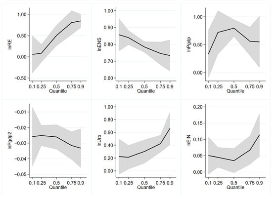
Figure 8.
Coefficient change for each variable in two-step quantile regression.
As shown in Table 8, the influences of different variables on CO2 emissions exhibit significant heterogeneity. More specifically, at the 10th and 25th quantiles, the coefficient of the RE is not significant, but becomes significant at higher quantiles with an obvious increase in coefficient size. This implies that the marginal decrease in the RE in the provinces located at higher quantiles (i.e., 50th, 75th, and 90th) promotes a greater CO2 reduction than that in the provinces located at the lower quantiles, which supports the findings of the regional heterogeneity analysis in Section 5.1. In terms of the control variables, an inverted-U-type nexus still exists between per capita income and CO2 emissions, except at the 10th quantile. The coefficients of energy structure (lnENS), urbanization (lnUrb), and trade openness (lnTra) at all quantiles are statistically significant, and the signs are consistent with the benchmark estimation results, as discussed in Section 4.2.3. This indicates CO2 emissions in China are significantly affected by energy structure, urbanization, and trade openness at all quantile levels.
Notably, an interesting finding can be seen from Figure 8, namely, that the energy structure coefficient shows a downward trend in all quantiles. This implies that the impact of the energy structure (measured by coal′s share of total energy consumption) on CO2 emissions is gradually weakening. The reason for this may be that, in recent decades, the central government of China implemented a series of policies, such as applying structural reforms to the supply side of the energy sector and prioritizing the development of renewable energy industries. As a result, the proportion of traditional fossil energy gradually declined, thus weakening the positive role of the energy structure on CO2 emissions.
5.3. Panel Causality Analysis
To enable more precise and targeted energy policies to be drawn up, we further conducted causal relationship checks for all variables based on the D-H panel causality test, which was proposed by Dumitrescu and Hurlin [76]. Table 9 shows the results. In addition, to clearly identify the causal relationship between variables, we also plotted the causality relationship flow, as shown in Figure 9.
Table 9.
Results of the D-H panel causality test.
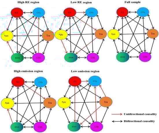
Figure 9.
Causality relationship flow across different regions.
Specifically, for the full sample, bidirectional causality was detected between variables, including the RE and CO2 emissions, which again supports the significant impacts of the RE on CO2 emissions, as shown in Section 4.2.3. In addition, the bidirectional causality among all of the four control variables (i.e., ENS, Pgdp, Urb, Tra) and CO2 emissions verified the robustness of the regression results presented in Section 5.3. Moreover, it was observed that there is heterogeneous causality link among the variables across the four regions. In the high-RE and high-emission regions, the RE and CO2 emissions exhibit a significant bidirectional causal relationship. Nevertheless, one-way causality from the RE to CO2 emissions exists in the low-RE and low-emission regions. This implies full consideration should be given to the regional differences when formulating RE and emission reduction policies for each region by effectively controlling the influence channels.
6. Conclusions
The existence of an RE poses a potential challenge to energy-saving and emission-reduction goals that solely rely on improvements in energy efficiency. In the context of lowering carbon emissions, attention should be paid to the RE in terms of its adverse impact on the environment. To understand the potential impacts of the RE on greenhouse gases, we attempted to evaluate the China’s provincial RE values over the period 2001–2017, for the short and long run, and to explore the extent to which RE contributes to the increment in CO2 emissions. Considering regional heterogeneity, asymmetric and regional heterogeneity analyses were further conducted. The main conclusions are as follows.
First, based on the calculation results of this study, China’s national average rebound level was 90.47% in the short run, and 78.17% in the long run, during the 2001–2017 period. Most of the provinces experienced a partial RE, whereas some provinces experienced a backfire effect, such as Guangxi and Henan. Furthermore, the RE in the short run was greater than that in the long run for the whole sample. Most of the provinces having high energy rebounds were concentrated in the central and eastern regions.
Second, the empirical results indicate that an increase in the short-run RE leads to an increment in CO2 emissions of approximately 0.818%, whereas a 1% increase in the long-run RE leads to an increment in CO2 emissions of approximately 0.695%. Accordingly, reducing the RE can mitigate China’s CO2 emissions. With respect to the regional heterogeneity analysis, the CO2 emissions in each of the four types of region (e.g., high-emission region, low-emission region, high-RE region, and low-RE region), particularly the high-emission and high-RE regions, are significantly and positively affected by the RE.
Third, the asymmetric analysis implies that a marginal decrease in the RE in the provinces located at higher quantiles (i.e., 50th, 75th, and 90th) promotes a greater CO2 reduction than that in the provinces located at lower quantiles. In addition, the energy structure exerts a gradually reducing impact on CO2 emissions across all quantiles. The D-H panel causality test indicates there is a heterogeneous causality link among the variables across the four regions. In the high-RE and high-emission regions, the RE and CO2 emissions have a significant bidirectional causal relationship. Nevertheless, one-way causality exists from the RE to CO2 emissions in the low-RE and low-emission regions.
Notably, this study only examined the preliminary empirical relationship between the rebound effect and CO2 emissions, and is subject to some limitations. One limitation is associated with the specific influence mechanism in the rebound effect–CO2 emissions relationship. Exploring how the rebound effect influences CO2 emissions can help policymakers to accurately formulate specific strategies. Thus, in future research, we will discuss the internal direct and indirect impact mechanisms between the rebound effect and CO2 emissions.
Author Contributions
Conceptualization, Q.J. and X.D.; methodology, C.D.; software, M.A.; validation, Q.J., X.D. and C.D.; formal analysis, Q.J.; investigation, M.A.; resources, C.D.; data curation, M.A.; writing—original draft preparation, M.A.; writing—review and editing, M.A.; visualization, C.D.; supervision, Q.J.; project administration, X.D.; funding acquisition, Q.J. All authors have read and agreed to the published version of the manuscript.
Funding
This research was founded by Research Funds for the Central Universities in UIBE (NO. 21YB06).
Conflicts of Interest
The authors declare no conflict of interest.
Abbreviations
| RE | Energy rebound effect | GDP | Gross domestic product |
| DEPI | Dynamic comprehensive energy efficiency index | CEADs | China Emission Accounts and Database |
| Mtce | Million tonnes coil equivalent | CSY | China Statistical Yearbook |
| EKC | Environmental Kuznets curve | CESY | China Energy Statistical Yearbook |
| CADF | Cross-sectionally augmented Dickey–Fuller | D-GMM | Differential generalized method of moments |
| CD | Cross-section dependence | SYS-GMM | System generalized method of moments |
| Effch | Energy efficiency change | Tech | Technological progress change |
| k | Capital stock | L | Labor |
| CIPS | Cross-sectionally augmented Im, Pesaran, and Shin | CO2 | Carbon dioxide |
Appendix A
Table A1.
Descriptions and data sources of the variables.
Table A1.
Descriptions and data sources of the variables.
| Variable | Definition | Data Sources |
|---|---|---|
| RE | Energy rebound effect | Calculation in Section 4.1 |
| CO2 | CO2 emissions of each province | China Emission Accounts and Database |
| GDP | Gross domestic product (GDP) of each province | CSY (2018) |
| P | Energy price (P) was measured by the price index of fuels | CSY (2018) |
| E | Total energy consumption of each province | CESY (2018) |
| K | Capital input (K) was calculated based on the perpetual inventory method | CSY (2018) |
| L | Labor input (L) was measured by employee number of each province at the end of the year | CSY (2018) |
| DEPI | Dynamic comprehensive energy efficiency index | Calculation in Section 4.1 |
| Pgdp | Per capita gross domestic product (GDP) of each province | CSY (2018) |
| ENS | Energy structure (ENS) was measured by coal consumption as a percentage of total energy consumption | CESY (2018) |
| Urb | Urbanization (Urb) was calculated by the ratio of permanent urban population to total population | CSY (2018) |
| Tra | Trade openness (Tra) was presented as the ratio of net trade imports and exports to the aggregate GDP | CSY (2018) |
References
- Foumani, M.; Smith-Miles, K. The impact of various carbon reduction policies on green flowshop scheduling. Appl. Energy 2019, 249, 300–315. [Google Scholar] [CrossRef]
- Benjaafar, S.; Li, Y.; Daskin, M. Carbon footprint and the management of supply chains: Insights from simple models. IEEE Trans. Autom. Sci. Eng. 2013, 10, 99–116. [Google Scholar] [CrossRef]
- Cansino, J.M.; Ordonez, M.; Prieto, M. Decomposition and measurement of the rebound effect: The case of energy efficiency improvements in spain. Appl. Energy 2022, 306, 117961. [Google Scholar] [CrossRef]
- Lin, B.; Zhu, P. Measurement of the direct rebound effect of residential electricity consumption: An empirical study based on the china family panel studies. Appl. Energy 2021, 301, 117409. [Google Scholar] [CrossRef]
- Böhringer, C.; Rivers, N. The energy efficiency rebound effect in general equilibrium. J. Environ. Econ. Manag. 2021, 109, 102508. [Google Scholar] [CrossRef]
- Fowlie, M.; Greenstone, M.; Wolfram, C. Do energy efficiency investments deliver? Evidence from the weatherization assistance program. Q. J. Econ. 2018, 133, 1597–1644. [Google Scholar] [CrossRef]
- CESY; National Bureau of Statistics. China Energy Statistical Yearbook 2020. 2020. Available online: http://www.Stats.Gov.Cn/ (accessed on 18 January 2021).
- CEADs. China Emission Accounts and Datasets. 2020. Available online: https://www.Ceads.Net.Cn/ (accessed on 25 January 2021).
- Bye, B.; Faehn, T.; Rosnes, O. Residential energy efficiency policies: Costs, emissions and rebound effects. Energy 2018, 143, 191–201. [Google Scholar] [CrossRef]
- Saunders, H.D. Recent evidence for large rebound: Elucidating the drivers and their implications for climate change models. Energ. J. 2015, 36, 23–48. [Google Scholar] [CrossRef]
- Adetutu, M.O.; Glass, A.J.; Weyman-Jones, T.G. Economy-wide estimates of rebound effects: Evidence from panel data. Energy J. 2016, 37, 251–269. [Google Scholar] [CrossRef]
- Wei, T.Y.; Zhou, J.J.; Zhang, H.X. Rebound effect of energy intensity reduction on energy consumption. Resour. Conserv. Recycl. 2019, 144, 233–239. [Google Scholar] [CrossRef]
- De Rocha, F.F.; de Almeida, E.L.F. A general equilibrium model of macroeconomic rebound effect: A broader view. Energy Econ. 2021, 98, 105232. [Google Scholar] [CrossRef]
- Shao, S.; Huang, T.; Yang, L. Using latent variable approach to estimate china’s economy-wide energy rebound effect over 1954–2010. Energy Policy 2014, 72, 235–248. [Google Scholar] [CrossRef]
- Shahbaz, M.; Tiwari, A.K.; Nasir, M. The effects of financial development, economic growth, coal consumption and trade openness on CO2 emissions in south africa. Energy Policy 2013, 61, 1452–1459. [Google Scholar] [CrossRef]
- Farhani, S.; Chaibi, A.; Rault, C. CO2 emissions, output, energy consumption, and trade in tunisia. Econ. Modelling 2014, 38, 426–434. [Google Scholar] [CrossRef]
- Jevons, W. The Coal Question; An inquiry Concerning the Progress of the Nation, and the Probable Exhaustion of Our Coal-Mines; Macmillan Co.: London, UK, 1865; Volume 1, pp. 1–323. [Google Scholar]
- Daniel Khazzoom, J. Economic implications of mandated efficiency in standards for household appliances. Energy J. 1980, 1, 21–40. [Google Scholar] [CrossRef]
- Brookes, L. Energy efficiency fallacies revisited. Energy Policy 2000, 28, 355–366. [Google Scholar] [CrossRef]
- Brockway, P.E.; Sorrell, S.; Semieniuk, G.; Heun, M.K.; Court, V. Energy efficiency and economy-wide rebound effects: A review of the evidence and its implications. Renew. Sustain. Energy Rev. 2021, 141, 110781. [Google Scholar] [CrossRef]
- Anson, S.; Turner, K. Rebound and disinvestment effects in refined oil consumption and supply resulting from an increase in energy efficiency in the scottish commercial transport sector. Energy Policy 2009, 37, 3608–3620. [Google Scholar] [CrossRef]
- Hanley, N.; McGregor, P.G.; Swales, J.K.; Turner, K. Do increases in energy efficiency improve environmental quality and sustainability? Ecol. Econ. 2009, 68, 692–709. [Google Scholar] [CrossRef]
- Yan, Z.; Ouyang, X.; Du, K. Economy-wide estimates of energy rebound effect: Evidence from china’s provinces. Energy Econ. 2019, 83, 389–401. [Google Scholar] [CrossRef]
- Barker, T.; Dagoumas, A.; Rubin, J. The macroeconomic rebound effect and the world economy. Energy Effic. 2009, 2, 411–427. [Google Scholar] [CrossRef]
- Lin, B.Q.; Liu, X. Dilemma between economic development and energy conservation: Energy rebound effect in china. Energy 2012, 45, 867–873. [Google Scholar] [CrossRef]
- Felipe, J.; McCombie, J.S.L. What is wrong with aggregate production functions. On temple’s aggregate production functions and growth economics’. Int. Rev. Appl. Econ. 2010, 24, 665–684. [Google Scholar] [CrossRef]
- Temple, J. Aggregate production functions and growth economics. Int. Rev. Appl. Econ. 2006, 20, 301–317. [Google Scholar] [CrossRef]
- Du, H.; Chen, Z.; Zhang, Z.; Southworth, F. The rebound effect on energy efficiency improvements in china’s transportation sector: A cge analysis. J. Manag. Sci. Eng. 2020, 5, 249–263. [Google Scholar] [CrossRef]
- Qiu, Y.; Kahn, M.E.; Xing, B. Quantifying the rebound effects of residential solar panel adoption. J. Environ. Econ. Manag. 2019, 96, 310–341. [Google Scholar] [CrossRef]
- Shao, S.; Guo, L.; Yu, M.; Yang, L.; Guan, D. Does the rebound effect matter in energy import-dependent mega-cities? Evidence from shanghai (china). Appl. Energy 2019, 241, 212–228. [Google Scholar] [CrossRef]
- Liu, H.; Ren, Y.; Wang, N. Energy efficiency rebound effect research of china’s coal industry. Energy Rep. 2021, 7, 5475–5482. [Google Scholar] [CrossRef]
- Meng, M.; Li, X. Evaluating the direct rebound effect of electricity consumption: An empirical analysis of the provincial level in china. Energy 2022, 239, 122135. [Google Scholar] [CrossRef]
- Zhang, S.; Lin, B. Investigating the rebound effect in road transport system: Empirical evidence from china. Energy Policy 2018, 112, 129–140. [Google Scholar] [CrossRef]
- Du, K.; Shao, S.; Yan, Z. Urban residential energy demand and rebound effect in china: A stochastic energy demand frontier approach. Energy J. 2021, 42, 175–193. [Google Scholar] [CrossRef]
- Li, J.; Lin, B. Rebound effect by incorporating endogenous energy efficiency: A comparison between heavy industry and light industry. Appl. Energy 2017, 200, 347–357. [Google Scholar] [CrossRef]
- Zhang, J.; Lawell, L.C.Y.C. The macroeconomic rebound effect in china. Energy Econ. 2017, 67, 202–212. [Google Scholar] [CrossRef]
- Shahbaz, M.; Solarin, S.A.; Mahmood, H.; Arouri, M. Does financial development reduce CO2 emissions in malaysian economy? A time series analysis. Econ. Model. 2013, 35, 145–152. [Google Scholar] [CrossRef]
- Esteve, V.; Tamarit, C. Threshold cointegration and nonlinear adjustment between CO2 and income: The environmental kuznets curve in spain, 1857–2007. Energy Econ. 2012, 34, 2148–2156. [Google Scholar] [CrossRef]
- Haisheng, Y.; Jia, J.; Yongzhang, Z.; Shugong, W. The impact on environmental kuznets curve by trade and foreign direct investment in china. Chin. J. Popul. Resour. Environ. 2005, 3, 14–19. [Google Scholar] [CrossRef]
- Iwata, H.; Okada, K.; Samreth, S. Empirical study on the environmental kuznets curve for CO2 in france: The role of nuclear energy. Energy Policy 2010, 38, 4057–4063. [Google Scholar] [CrossRef]
- Plassmann, F.; Khanna, N. Household income and pollution. J. Environ. Dev. 2016, 15, 22–41. [Google Scholar] [CrossRef]
- Zilio, M.; Recalde, M. Gdp and environment pressure: The role of energy in latin america and the caribbean. Energy Policy 2011, 39, 7941–7949. [Google Scholar] [CrossRef]
- Day, K.M.; Grafton, R.Q. Growth and the environment in canada: An empirical analysis. Can. J. Agric. Econ. 2003, 51, 197–216. [Google Scholar] [CrossRef]
- Feng, T.; Sun, L.; Zhang, Y. The relationship between energy consumption structure, economic structure and energy intensity in china. Energy Policy 2009, 37, 5475–5483. [Google Scholar] [CrossRef]
- Xu, G.Y.; Schwarz, P.; Yang, H.L. Adjusting energy consumption structure to achieve china’s CO2 emissions peak. Renew. Sust. Energ. Rev. 2020, 122, 109737. [Google Scholar] [CrossRef]
- Wang, J.; Yu, S.; Liu, T. A theoretical analysis of the direct rebound effect caused by energy efficiency improvement of private consumers. Econ. Anal. Policy 2021, 69, 171–181. [Google Scholar] [CrossRef]
- Martínez-Zarzoso, I.; Maruotti, A. The impact of urbanization on CO2 emissions: Evidence from developing countries. Ecol. Econ. 2011, 70, 1344–1353. [Google Scholar] [CrossRef]
- Shahbaz, M.; Loganathan, N.; Muzaffar, A.T.; Ahmed, K.; Ali Jabran, M. How urbanization affects CO2 emissions in malaysia? The application of stirpat model. Renew. Sustain. Energy Rev. 2016, 57, 83–93. [Google Scholar] [CrossRef]
- Fan, Y.; Liu, L.C.; Wu, G.; Wei, Y.M. Analyzing impact factors of CO2 emissions using the stirpat model. Environ. Impact Assess. Rev. 2006, 26, 377–395. [Google Scholar] [CrossRef]
- Liddle, B.; Lung, S. Age-structure, urbanization, and climate change in developed countries: Revisiting stirpat for disaggregated population and consumption-related environmental impacts. Popul. Environ. 2010, 31, 317–343. [Google Scholar] [CrossRef]
- Mutascu, M. A time-frequency analysis of trade openness and CO2 emissions in france. Energy Policy 2018, 115, 443–455. [Google Scholar] [CrossRef]
- Frankel, J.; Rose, A. An estimate of the effect of common currencies on trade and income. Q. J. Econ. 2002, 117, 437–466. [Google Scholar] [CrossRef]
- Hossain, M.S. Panel estimation for CO2 emissions, energy consumption, economic growth, trade openness and urbanization of newly industrialized countries. Energy Policy 2011, 39, 6991–6999. [Google Scholar] [CrossRef]
- Wójcik-Jurkiewicz, M.; Czarnecka, M.; Kinelski, G.; Sadowska, B.; Bilińska-Reformat, K. Determinants of decarbonisation in the transformation of the energy sector: The case of poland. Energies 2021, 14, 1217. [Google Scholar] [CrossRef]
- Drożdż, W.; Kinelski, G.; Czarnecka, M.; Wójcik-Jurkiewicz, M.; Maroušková, A.; Zych, G. Determinants of decarbonization—how to realize sustainable and low carbon cities? Energies 2021, 14, 2640. [Google Scholar] [CrossRef]
- Saunders, H.D. A view from the macro side: Rebound, backfire, and khazzoom–brookes. Energy Policy 2000, 28, 439–449. [Google Scholar] [CrossRef]
- CSY. China Statistical Yearbook 2018. Available online: https://data.cnki.net/Yearbook/Single/N2018110025 (accessed on 1 February 2021).
- CESY. China Energy Statistical Yearbook 2018. Available online: https://g.wanfangdata.com.cn/index.html (accessed on 8 February 2021).
- Boyd, G.A.; Pang, J.X. Estimating the linkage between energy efficiency and productivity. Energy Policy 2000, 28, 289–296. [Google Scholar] [CrossRef]
- Wu, F.; Fan, L.W.; Zhou, P.; Zhou, D.Q. Industrial energy efficiency with CO2 emissions in china: A nonparametric analysis. Energy Policy 2012, 49, 164–172. [Google Scholar] [CrossRef]
- Orea, L.; Llorca, M.; Filippini, M. A new approach to measuring the rebound effect associated to energy efficiency improvements: An application to the us residential energy demand. Energy Econ. 2015, 49, 599–609. [Google Scholar] [CrossRef]
- CSY. China Statistical Yearbook 2020. 2020. Available online: http://edu.macrochina.com.cn (accessed on 15 February 2021).
- Grossman, G.M.; Krueger, A.B. Economic growth and the environment. Q. J. Econ. 1995, 110, 353–377. [Google Scholar] [CrossRef]
- Dong, K.; Jiang, Q.; Shahbaz, M.; Zhao, J. Does low-carbon energy transition mitigate energy poverty? The case of natural gas for china. Energy Econ. 2021, 99, 105324. [Google Scholar] [CrossRef]
- Pesaran, M.H. General Diagnostic Tests for Cross Section Dependence in Panels; IZA Discussion Paper No. 1240; Institute for the Study of Labor: Bonn, Germany, 2004. [Google Scholar]
- Breusch, T.S.; Pagan, A.R. The lagrange multiplier test and its applications to model specification in econometrics. Rev. Econ. Stud. 1980, 47, 239–253. [Google Scholar] [CrossRef]
- Friedman, M. The use of ranks to avoid the assumption of normality implicit in the analysis of variance. J. Am. Stat. Assoc. 1937, 32, 675–701. [Google Scholar] [CrossRef]
- Frees, E.W. Longitudinal and Panel Data: Analysis and Applications in the Social Sciences; Cambridge University Press: Cambridge, UK, 2004. [Google Scholar]
- Pesaran, M.H. A simple panel unit root test in the presence of cross-section dependence. J. Appl. Econom. 2007, 22, 265–312. [Google Scholar] [CrossRef]
- Zhao, J.; Jiang, Q.; Dong, X.; Dong, K. Would environmental regulation improve the greenhouse gas benefits of natural gas use? A chinese case study. Energy Econ. 2020, 87, 104712. [Google Scholar] [CrossRef]
- Arellano, M.; Bover, O. Another look at the instrumental variable estimation of error-components models. J. Econ. 1995, 68, 29–51. [Google Scholar] [CrossRef]
- Lin, B.; Zhu, J. Impact of china’s new-type urbanization on energy intensity: A city-level analysis. Energy Econ. 2021, 99, 105292. [Google Scholar] [CrossRef]
- Saboori, B.; Sulaiman, J.; Mohd, S. Economic growth and CO2 emissions in malaysia: A cointegration analysis of the environmental kuznets curve. Energy Policy 2012, 51, 184–191. [Google Scholar] [CrossRef]
- Dong, K.; Ren, X.; Zhao, J. How does low-carbon energy transition alleviate energy poverty in China? A nonparametric panel causality analysis. Energy Econ. 2021, 103, 105620. [Google Scholar] [CrossRef]
- Sun, H.P.; Clottey, S.A.; Geng, Y.; Fang, K.; Amissah, J.C.K. Trade openness and carbon emissions: Evidence from belt and road countries. Sustainability 2019, 11, 2682. [Google Scholar] [CrossRef]
- Dumitrescu, E.I.; Hurlin, C. Testing for granger non-causality in heterogeneous panels. Econ. Model. 2012, 29, 1450–1460. [Google Scholar] [CrossRef]
Publisher’s Note: MDPI stays neutral with regard to jurisdictional claims in published maps and institutional affiliations. |
© 2022 by the authors. Licensee MDPI, Basel, Switzerland. This article is an open access article distributed under the terms and conditions of the Creative Commons Attribution (CC BY) license (https://creativecommons.org/licenses/by/4.0/).