Article

AI Energy Optimal Strategy on Variable Speed Drives for Multi-Parallel Aqua Pumping System

by
Manickavel Baranidharan
1 and
Rassiah Raja Singh
2,*
1
School of Electrical Engineering, Vellore Institute of Technology, Vellore 632014, India
2
Department of Energy and Power Electronics, Vellore Institute of Technology, Vellore 632014, India
*
Author to whom correspondence should be addressed.
Energies 2022, 15(12), 4343; https://doi.org/10.3390/en15124343
Submission received: 19 April 2022 / Revised: 23 May 2022 / Accepted: 24 May 2022 / Published: 14 June 2022
(This article belongs to the Special Issue Research on the Optimal Selection of Electromechanical Drives)

Abstract

:
In the industrial world, parallel pump systems are frequently employed. Due to various reasons, the pumps are frequently operated outside their intended parameters, which reduces their efficiency and performance. To operate the pump system with optimum efficiency, the pumps and their speed selection are mandatory. This research presents an optimum switching technique for variable speed pumping stations with multi-parallel pump combinations to enhance energy savings. The proposed optimal control system is designed in such a way as to decrease overall losses in the pump system. The effectiveness of the proposed method is investigated on a real scale of a multi-parallel pump drive system in a Matlab Simulink environment, and experimental validation is performed in a laboratory prototype. The suggested approach enhances power savings and shall be adapted for various pumping applications.

1. Introduction

Industrial development is the major driving force for building the Nation. The industry transforms raw materials into goods that are more desirable to individuals through various process activities. Depending upon industrial applications, various stages are involved, including electrical, mechanical, chemical, and thermal operations. Pumping is an important application in various industries, especially in process industries [1]. Pumps consume between 20% and 25% of the world’s total power usage, according to data [2,3]. The pump system consists of suction and pressure for lifting and transferring the liquids, respectively. In the early 1900s, the mechanical engine-driven pump was used, where the output was controlled by a throttle mechanism and sluice gate control. Alternatively, the output is regulated by varying the shaft speed through gear ratios, belts, and pulleys on the pump drive train [4]. In the later 1900s, electric motor-driven pumps gradually appeared, and in recent times, the pumping industry has been dominated by electric motors [5]. Moreover, the classical regulation methods are adapted to control the output of an electrically driven pump. However, this approach causes energy wastage over the flow constraint barrier [6]. In modern times, the technologies gradually made many improvements to the electrical pump drive systems. The adaptation of variable speed technology to enhance the pump drive performance and efficiency creates a milestone in pumping technology [7]. The variable speed drive technology varies pump speed and matches the load requirement. These operations use the energy optimally with respect to the demand pattern. This energy consumption is considerably decreased when Variable speed drives (VSD) technology is used, allowing the same production to be operated with significantly less energy. Parallel pumps are commonly employed in a variety of applications, including those requiring a high flow rate or pressure, as well as those requiring a broad range of demand fluctuations. In relation to life cycle price, consistency, also protection, the benefits then drawbacks of a single pump vs. a multi-pump operation are compared, with the result that a multi-pump operation is typically safer and more cost-effective [8]. However, optimal control methods for precisely controlling the energy-saving effect in pumping stations are still lagging. Intelligent pump control goes beyond maximizing the individual drive’s capabilities.
Pumps powered by artificial intelligence provide significant environmental and economic benefits. It tracks and regulates energy use, lowering it during peak hours, recognizing and reporting problems, and anticipating equipment failures. It has the ability to compress and analyze large amounts of data, making it valuable for monitoring and understanding data provided by the energy industry in order to minimize energy use. The anfis is a single system that mixes artificial neural network (ANN) among Fuzzy inference systems (FIS). An anfis has a number of benefits, along with the capacity to display a system’s dynamic creation, flexibility, and speed of development. Its inference algorithm is built on a collection of fuzzy if-then rules that can adapt to predict nonlinear functions. As a function of this, anfis is referred to as a global estimator. The evolutionary algorithm’s optimum parameters can be employed to make the anfis extra effective and more perfect. When employing fuzzy logic to address an issue, there is no one-size-fits-all method. It is not usually universally accepted due to inaccuracy in findings. Another important disadvantage of fuzzy logic control systems is that they rely entirely on human knowledge and skill. Machine learning or neural networks are not identified by these algorithms. This anfis approach combines mathematical and linguistic skills. Anfis also makes use of the ANN’s ability to categorize data and find patterns. The anfis model is easier to understand than the ANN model, and it produces fewer memory errors. A statistical approach and computational method for connecting inputs and outputs is the artificial neural network. Anfis is a method that blends ANN with FIS. ANN might be used with FIS to expand modeled system execution, fault tolerance, and flexibility. Variable frequency drives, also described as adjustable speed drives, are electrical and mechanical systems that change the voltage and frequency to alter the AC motor N-T characteristics. Variable frequency drive (VFD) consumption has risen at an alarming rate in recent decades, making the sector more energy efficient because motor applications consume 25% of total energy. VFD systems minimize system size and increase the achievement of semiconductor technology, software, and hardware power switches and drive schemes. The configurations for VFD are AC-AC and DC-DC. Induction motor speed control is more cost-effective, easy, dependable, and precise. It allows for constant systems integration across a wide speed range. VFDs not only manage the speed of induction motors but also make them start more smoothly by lowering the inrush current and increasing the power factor. As a result, electricity usage is lowered as well. Pumps come in three different types: axial flow, centrifugal flow, and positive displacement. The path of fluid flow in centrifugal pumps varies by 90 degrees as it passes through the impeller, although the path of movement in axial flow pumps remains unchanged. The frequency and voltage of an electric motor’s power supply are controlled using a VFD. The motor’s ramp-up and ramp-down, as well as start and stop, could be controlled by the VFD. Despite the fact that the drive controls the frequency and voltage of the power supplied to the motor, we frequently refer to it as speed control because the outcome is a change in motor speed. The types of control techniques are classified into voltage/frequency (v/f), voltage vector control plus (vvc+), flux sensor less, and flux w/motor feedback.
It links and integrates drives in pumping applications, allowing them to function at peak efficiency and save up to 20% more than “traditional” drives. The highest levels of availability are also provided by the high degrees of redundancy. For instance, lead and lag pumps are often operated together when process flow rate requirements can be met by a single pump. This can result from a common belief that by operating three similar pumps in parallel, the flow rate is increased. While flow rate is increased by parallel operation, it also causes higher fluid friction losses, contributes to higher discharge pressure, decreases the flow rate given by each pump, and changes the efficiency of each pump. Furthermore, to move a given fluid volume, more energy is needed [9]. In addition, the head vs. flow rate for parallel operation by adding a flow value at the same head, the H-Q curve of pumps operating in parallel can be constructed with a system curve. The operating point of pumps operating in parallel depends on the device curve, in particular the proportion of the characteristics of the static head. Operation of three pumps in parallel in the piping method, with friction losses in particular. In the graph, it can be observed that the addition of each next pump raises total flow at the lowest flow value—Q1, Q2, and Q3. In this work, we demonstrate experimentally a simulation for an optimum switching technique in variable speed pumping stations with identical parallel pumps and also present that energy saving could be reached based on these setpoint values with varying flowrate. So, the optimal control strategy is created and such a way as to decrease the overall losses of the proposed pump drive system and increase the pump reliability. The main contributions of this paper are that in single pump operating for the full load condition, it consumes the power is more also the same load condition in two parallel pumps using it consumes less power compared to a single pump operation. Meanwhile, in three parallel pump connections for the same full load condition, it consumes very less power; also, it saves energy by comparing the single parallel pump also using two parallel pumps. The remaining of this paper is ordered as follows. Initially, introduce pump importance and industry, and the modeling equations of centrifugal pump and the induction motor are exhibited in Section 2. In Section 3, the methodology of the experiment with the parallel pump arrangements is discussed. In Section 4, we are developing the simulation model for the parallel pumping system by MATLAB software with the Anfis technique and experimental setup also, the parallel pumping system explanation in Section 4, and the corresponding results and discussion in Section 5. Finally, we end with the conclusions in Section 6.

2. Modeling of Intelligent Aqua Pump Drive System

To build this pump drive system and to evaluate the model performance, The centrifugal pump and induction motor are mathematically modeled.

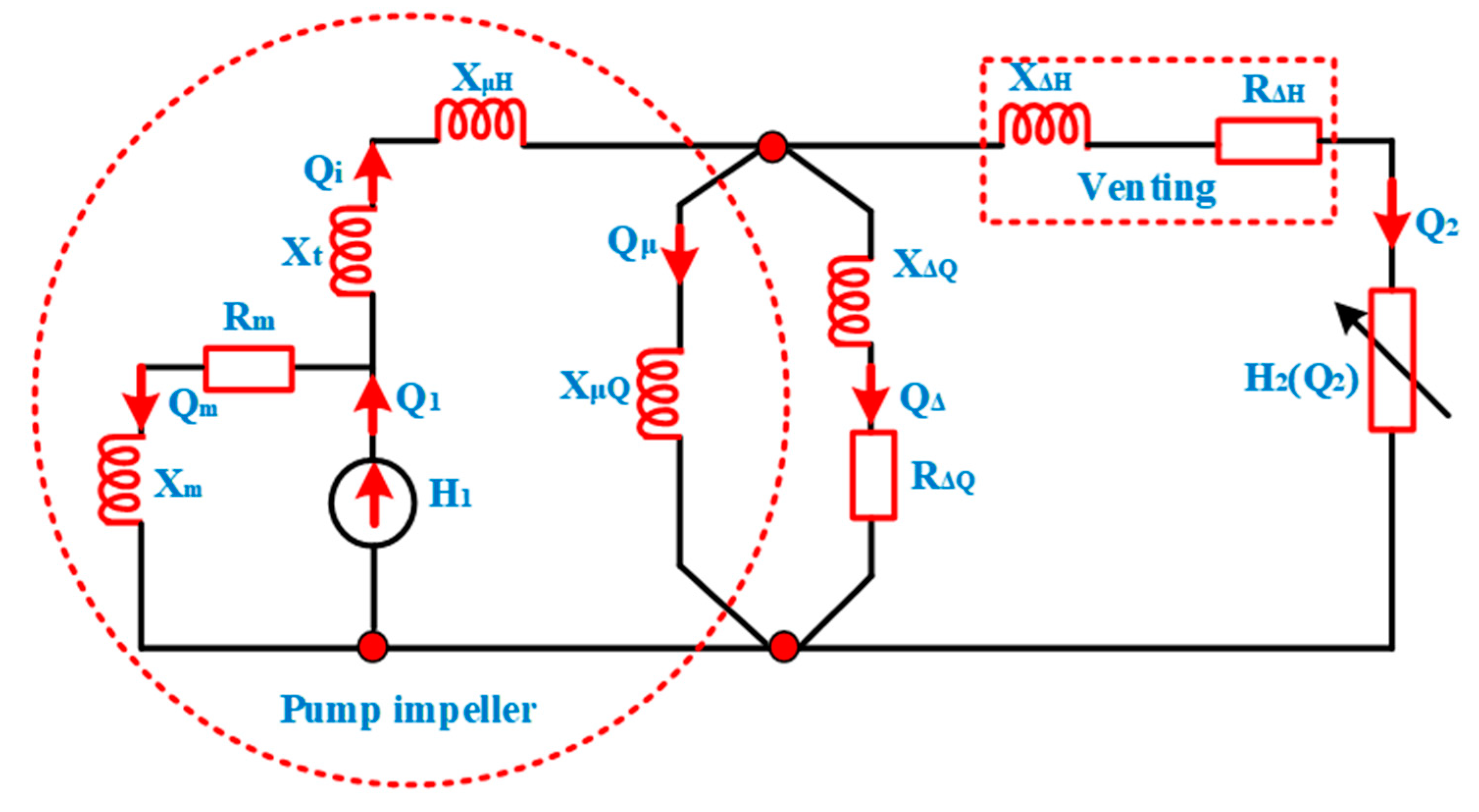
2.1. Mathematical Modeling of Aqua Pump

The torque on the axis determines angular acceleration as stated by newton’s law of force’s equivalent. As a result, the motor pump set’s equation of motion is as follows:
J d ω dt = M a M p = M MT ( M p + M ς )
where: J is the moment of inertia (in a specific case, it is the constant of proportionality, J = const.), MMT is the active torque from the asynchronous motor, MP is the passive/resistive torque of the pump, and Mζ is the viscous torque. The asynchronous motor torque is represented by the following equation, considering that the number of stator poll pairs is one and that the network frequency is f:
M MT = k MT U 2 ( 2 π f ω )
Equation (2) The viscous torque Mζ and the pump’s passive torque Mp are calculated as follows:
M ζ = k ζ ω
M P = ρ gq v 2 H η p ω
The basic characteristics of a centrifugal pump are from Equation (4): the tank constantly receives water with input flow qv1. The output water flow through the control valve is qv2, H is the pump total head, then angular velocity ω. A peripheral cross-section of the impeller channels and the meridian module of velocity can be used to express pump flow. According to the pump affinity law, the flow rate is proportional to the speed; also, the head is proportional to the speed square, and the power is proportional to the speed cube. As a result, it is suitable for many modes of operation.
Q 1 Q 2 = N 1 N 2   and   H 1 H 2 = N 1 2 N 2 2 ( or ) ω 1 2 ω 2 2     and   P 1 P 2 = N 1 3 N 2 3
It is important to note that the calculation assumes a constant pump efficiency coefficient. It is fundamentally altered in different modes, which has an effect on the settings to some extent and reflects the parameters.
Because Equation (5) is applicable for any two modes, it may be written for arbitrary and nominal modes and substituted with (4):
M P = ρ gH N η p ω N 2 q v 2 ω = k P q v 2 ω
The centrifugal pump’s resistive torque is proportional to the output flow qv2 and the angular velocity ω.
Specifically, the centrifugal pump’s resistive torque is proportional to the out flow qv2 and the rotational velocity. Pump characteristics are specified by pump manufacturers at a nominal speed n. Because of the difficulty of centrifugal pump dynamics, the concept such that the qv-H curve properly depicts the pump’s behavior in provisional management is recognized in their research, i.e., the pump’s static feature is employed. The equation can be used to explain the characteristic curve of a centrifugal pump.
H = A ω 2 + B ω q V + Cq V 2
The characteristic constants for each pump are A, B, and C. This formula determines the family of static characteristics of the centrifugal pump since it is a parabola family with parameters. The pump head will be as follows when qv and is expressed in nominal values:
P P 1 = ( A + B q vN ω N + C q vN 2 ω N 2 ) ω 2 = k ω ω 2
The pressure at the pump inlet may be determined by looking at how the pump and the suction pipeline work together. A pipeline pump will function in such a way that the energy essential to transport the fluid over the pipe is the same as the energy imparted to the liquid by the pump.
H potr = ρ gh gv + p p b + k c q v 2 2
Considering that the head (H) is the same as the difference in pressures at the pump’s input and outflow flanges in the same diameters, we get:
P = k ω ω 2 + p b ρ gh gv k c q v 2 2
If qv2 is the flow through the control valve, the pressure drop in the valve may be expressed.
q v 2 = A ( Y ) v v = k v A ( Y ) Δ p v = k v A ( Y ) p p 2
In the preceding equation, kv is the valve constant, and A(Y) is a nonlinear function that describes the change in the cross-section of the valve as the position of its spindle changes. The valve’s constructive data is used to determine this static feature [10].
q v 2 = k v Y ω 1 + k c k v 2 Y 2 . k ω ω 2 ρ gh gv + p b p 2
Based on the preceding, the centrifugal pump’s resistive torque may be accurately represented by the equation [8]:
M p = k p k v Y ω 1 + k c k v 2 Y 2 . k ω ω 2 ρ gh gv + p b p 2
The following expressions are used in the modeling: P is the number of pole pairs, p is pressure, P1 is pump 1, Pb is pump base water level, and p2 is pressure valve 2. It takes the following form when the derived expression for each torque is replaced by (8):
J d ω dt = ( 314 k MT U 2 k MT U 2 ω ) ( k p k v Y ω 1 + k c k v Y 2 . k ω ω 2 ρ gh gv + p b p 2 + k ζ ω )
Equation (14) is a nonlinear mathematical model of a centrifugal pump that is used in the plant.
The structure of the equivalent circuit of the centrifugal pump of Figure 1 also its modal organizes is: Rm, Xm—dissipative and reactive hydro-resistances, whether replicate mechanical energy wastage of the centrifugal pump (CP) impeller due to wheel friction and hydraulic braking; RΔH, XΔH—dissipative and reactive hydro-resistances, that replicate hydraulic head losses in the CP spiral venting; RΔQ, XΔQ—dissipative also reactive hydro-resistances, this replicates inspiration of feedback on the CP’s head; Xt—reactive hydro-resistance of the spiral part of the CP’s venting; XμH, XμQ—reactive hydro-resistances, which account for the influence of a finite number of the impeller’s blades on the pump’s pressure and volumetric fluid losses; H1 = (H1d + jH1q)—phasor of the ideal pump’s rated head in non-functional mode; Q1, Q2, Qm—matching phasors of rated volumetric fluid losses on the input of CP; H2(Q2) static head characteristics of the hydraulic network. It is simplified by converting delta—connected impedances to minimize the number of equations of state of CP:
Z 01 = R m + jX m   ;   Z 12 = j ( X t + X Δ H )
Z 02 = jX Δ Q ( R Δ Q + jX Δ Q ) ( R Δ Q + j ( X Δ Q + X Δ Q ) )
After changing the schematic and joining passive two-port devices in series,
Z 0 = Z 01 Z 02 Z Σ   ;   Z 1 = Z 01 Z 12 Z Σ   ;   Z 2 = Z 02 Z 12 Z Σ +   Z Δ H
where
Z Σ = Z 01 + Z 02 + Z 03
The following nominal values are used to create CP mathematical model equations in a nominal per unit system:
N cpn = ρ gH cpn Q cpn
Z cpn = ρ gH cpn Q cpn
where
  • H cpn , Q cpn —nominal head and volumetric loss of fluid in CP;
  • S cpn , Z cpn —nominal power and module of the hydraulic impedance of CP;
  • ρ , g —per unit density of fluid and gravitational constant.
The method of contour coordinates is used to create a mathematical model of CP in the complex plane. If the phasors of volumetric losses Q1 and Q2 are used as contour coordinates, CP’s mathematical equations are: for frequency-controlled CP correlations between the phasor H1 module, its projections on d-q axes, and relative angular velocity of impeller, an empirically proved theory of self-modeling (auto-modeling) of centrifugal hydro-machines is stated as:
H 1 d 2 + H 1 q 2     ω r 2 H 1 n = 0
where: H1n—nominal head of idealized CP in no-load mode and nominal angular velocity of the impeller ω r   = 1. On the basis of co-linearity of phasors of real head and actual losses, the following CP-hydraulic network relationships are proposed:
H 2 d R g 2 ( Q 2 d , Q 2 q ) Q 2 d = 0
H 2 q R g 2 ( Q 2 d , Q 2 q ) Q 2 q = 0
R g 2 ( Q 2 d , Q 2 q ) Q 2 H 2 = 0
where Q 2 = Q 2 d 2 + Q 2 q 2 —actual volumetric losses and H 2 = H 2 d 2 + H 2 q 2 —actual head of real CP; R g 2 ( Q 2 d , Q 2 q ) = H 2 ( Q 2 ) Q 2 —hydraulic resistance of hydraulic network, which is defined by its static head characteristics H 2 ( Q 2 ) . Mechanical power Ncp on the shaft of CP is expressed as:
N cp = Re ( H 2 , Q 2 * ) = H 2 d Q 2 d + H 2 q Q 2 q
Useful hydraulic power N2 at the output of CP is calculated from:
N 2 = Re ( H 1 , Q 1 * ) = H 1 d Q 1 d + H 1 q Q 1 q

2.2. Mathematical Modeling of Induction Motor Drive-Based VFD

2.2.1. Steady-State Analysis of Induction Motor Drive

The equations for the voltages of the stator and rotor in the form of a three-phase system
v abcs = r s i abcs + p λ abcs
v abcr = r r i abcr + p λ abcr
The space vector version of the voltage equations yields the AC induction motor model. The following equations represent the system model specified in the stationary coordinate system coupled to the stator. The ideal motor model is symmetrical and linear characteristics of magnetic circuits.
Because apparatus and electricity system characteristics are commonly assumed in Ω, percent, or p.u of a base impedance, describing the voltage and flux linkage equation by means of reactance, preferably inductances, is more straightforward.
v qd 0 s = r s i qd 0 s + ω λ dqs + p λ qd 0 s
v qd 0 r = r r i qd 0 s + ( ω ω r ) λ dqs + p λ qd 0 s
v qs = r s i qs + ω ω b ψ ds + p ω b ψ qs
v ds = r s i ds ω ω b ψ qs + p ω b ψ ds
v 0 s = r s i 0 s + p ω b ψ 0 s
For the squirrel cage induction motor,
  v   qr = 0 = r r i qr + ( ω ω r ) ω b   ψ   dr + p ω b   ψ   qr
  v   dr = 0 = r r i dr ( ω ω r ) ω b   ψ   qr + p ω b   ψ   dr
  v   0 r = r r i 0 r + p ω b   ψ   0 r
The inductive reactance is calculated using a base angular velocity of ωb.
ψ qs = L ls i qs + L M ( i qs + i qr )
ψ ds = L ls i ds + L M ( i ds + i dr )
ψ 0 s = L ls i 0 s
  ψ   qr =   L   lr   i   qr + L M ( i qs +   i   qr )
  ψ   dr =   L   lr   i   dr + L M ( i ds +   i   dr )
  ψ   0 r =   L   lr i 0 r
where ω r - is the rotor angular speed, r s , r r - is the stator and rotor resistance, L M - is the mutual inductance, ψ ds , ψ qs - is stator flux of d-axis and q-axis, ψ dr , ψ qr - is rotor flux of d-axis and q-axis and λ abcs , λ abcr - is the flux linkages of stator and rotor. Various estimation approaches may be used to determine resistance, inductance, flux linkage, and the angular frequency of an induction motor [11].
T e = 1.5 p ( ψ ds i qs ψ qs i ds )
For obtaining the secondary voltage also frequency, the analogous ckt illustrated above has eliminated the need for a slip. In conclusion, the system might be simplified by eliminating the ideal transformer directly addressing the rotor’s resistance and reactance to the primary. Figure 2 shows the simplified induction motor equivalent circuit. Multiply the mentioned values by k2, where k is the operative stator/rotor turns ratio.

2.2.2. Dynamic Analysis of Induction Motor Drive

The induction motor circuit model works for constant slip, but it also works for gradually variable slip, which is common in motor starting. Only if T > TL would the motor start, and it would attain a constant operating speed of ω0 at T = TL, the crossing point P of the two torque-speed characteristics. The perturbation approach may be used to verify that P is a stable operating point for the load-speed characteristic. If the speed exceeds ω0 for any reason, the machine-load combination decelerates and returns to the operational position (T − TL) < 0. If the speed falls below zero, the opposite occurs.
During the accelerating period
T T L = J d ω dt
where J = combined inertia of motor and load. Now
ω = ( 1 s ) ω s
Therefore, Equation (41) modified to
T T L = J ω s ds dt
when S1 = 1 and S2 = S0. Because the quantity 1/ (T − TL) is nonlinear practical integration is limited to 90% (or) 95%. S0 depends on the desired precision.
Starting on No-Load (TL = 0):
In this particular case, it is assumed that the machine and load friction torque TL = 0. Stator losses to be negligible (R1 = 0), the motor torque as obtained from equation assuming (3) is
T = 3 ω s . V TH 2 ( R 2 / s ) ( R TH + R 2 / s ) 2 + ( X TH + X 2 ) 2
T = 3 ω s . V TH ( r 2 / s ) ( r 2 / s ) 2 + ( X 1 + X 2 ) 2
In addition, from Equation (5)
T max = 3 ω s . 0.5 V TH 2 R TH + R TH + ( X TH + X 2 ) 2
T max = 3 ω s . 0.5 V TH 2 ( X 1 + X 2 )
At a slip of Equation (48)
s max ,   T = R 2 R TH 2 + ( X TH + X 2 ) 2
s max ,   T = r 2 X 1 + X 2
From Equations (4) and (5),
T T max = 2 [ ( r 2 / S ) X 1 + x 2 + X 1 + x 2 ( r 2 / S ) ]
Substituting Equation (49) in (50)
T T max = 2 S max , T S + S S max , T
Since TL is assumed to be zero, the motor torque itself is the accelerating torque. The time tA to go from slip s1 to s2 is obtained
t A = J ω s 2 T max [ S 1 2 S 2 2 2 s max ,   T + s max ,   T ln S 1 S 2 ]
The acceleration time for the machine to reach a steady speed from the start can be computed from Equation (51) with S1 = 1 and S2 = s,
t A = J ω s 2 T max [ 1 S 2 2 2 s max ,   T + s max ,   T ln 1 S ]
Optimum Smax, T for Minimum Acceleration Time:
To find the optimum value of Smax, T for the dynamic modeling of induction motor to have minimum acceleration time to reach s2 from S1, Equation (51) must be differentiated with respect to Smax, T and equated to zero. This gives
( S max ,   T ) opt = ( S 1 S 2 ) 2 2 ln ( S 1 / S 2 )
For minimum acceleration time for the machine to reach any slip s from the start, the optimum value of Smax, T is given by Equation (53) with S1 = 1 and S2 = s. Then
( S max ,   T ) opt = ( 1 s ) 2 2 ln ( 1 / s )
Further, to enable us to compute the optimum value of the rotor resistance to accelerate the machine to slip S2 from S1, Equation (53) is substituted in Equation (48), giving
( r 2 ) opt = ( X 1 + X 2 ) ( S max , T ) opt

2.3. Intelligent Controller for Pump Drive System

An adaptive neuro-fuzzy inference system (ANFIS) was created using the fuzzy toolkit in Matlab. A few of the features include a fuzzy inference system, Membership function (MF) for input and MF for output, rules viewer, then output area. The no of MFs and their variety are set by the user, and they may be changed. Sugeno is used by anfis, which allows for the change of MFs and their range. Reverse method or combination of opposite method and minimal square method techniques are used to train various frameworks. The optimization approach uses the overall deviation also the square of the real then projected output to compute various outlines. The key advantages of employing anfis are its time efficiency and ease of use. Because anfis does not require human expert information, it takes the least amount of time and is additionally basic in framework estimation and MFs optimization, adding to long-term sustainability. Anfis outline has two main stages: the Neural network (NN) stage and the design stage. The other step promotes a hazy master framework by allowing participants to fine-tune their involvement capacities. Using input and output data pairings, a FIS file will be created [12]. At a similar time, membership functions are tuned using the least-squares approach, a backpropagation algorithm, or a mixture of the two. Anfis uses a linear input variable and a nonlinear output variable. The knowledge basis for this system is formed by two fuzzy input-created if-then rules, which are described by the equation below. An adaptive neuro-fuzzy inference system (ANFIS) is a deep learning method that combines adaptive control, artificial neural networks, and fuzzy inference systems. ANFIS takes advantage of the ability of an artificial neural network (ANN) to categorize data and discover patterns. However, the ANFIS model is more transparent to the user and generates fewer memory mistakes.
Table 1 represents the different types of pump optimization algorithms with the application presented; also, based on the other optimization algorithm, the ANFIS algorithm is suitable for the multi-parallel pumping system for energy consumption with a conservation perspective. In addition, these types of adaptive neuro-fuzzy inference systems are energy conservation points of use. It mainly provides energy optimization on the industrial application drives.
To provide a soft computation paradigm, the anfis model integrates neural networks with fuzzy systems. As an outcome, a synergetic result occurs, combining the benefits of mutually systems in linear also nonlinear methods. ANFIS is a combination of FIS with ANN, incorporating the advantages of both in a single pattern, including trainability, optimizable connectionist pattern, and human skilled learning articulated in linguistic relations by means of if-then instructions. The primary problem in anfis is deciding the type of MF and its degree of membership; for that, if no clear result is present, then the model’s optimal structure is established by trial and error. The hybrid approach, which is a mix of the least-squares technique and the backpropagation technique, was used for training this structure of anfis for this purpose. ANFIS may be used to successfully determine the best connection between a set of input and output information. The Takagi–Sugeno ANN can create fuzzy rules from assumed input-output information; hence, the system is forever explainable in terms of fuzzy if-then instructions, unlike ANNs, wherever the information obtained via learning is divided in every network weight and might not be read by individuals [26]. IF-then rules are used to link the input and then output framework together. An MR of parboiled hulls was evaluated using fuzzy if-then rules in the current study. Anfis is a five-layered pattern this uses the fuzzy logic regulators to solve difficulties quickly while minimizing steady-state error. Fuzzification, multiplication, normalization, defuzzification, and summation are the functions of the five layers that make up the anfis model. Fuzzy systems also NN are suitable partners in the creation of smart systems. Whereas NN is a low-level computing framework that operates well with raw data, fuzzy logic is concerned with higher-level thinking. Fuzzy systems, on the other hand, do not have the ability to learn and change. A neuro-fuzzy structure in detail is an NN that executes the same tasks as a fuzzy inference framework. For instance, Roger Jang’s anfis stands a five-layer feedforward NN that contains a fuzzification layer, instruction layer, normalization layer, defuzzification layer, then a one summation network. Adaptive Neuro-Fuzzy Inference System employs a hybrid knowledge technique that incorporates both the least-squares analyzer also the gradient descent approach [27].
Figure 3 depicts the anfis logical architecture for the proposed system. Fuzzy if-then instructions may be included in an anfis system, as well as modification of the MF based on a required input-output data match. An enhanced approach for modeling and controlling complex engineering systems is ANFIS. Using the modeling benefits of the Sugeno fuzzy inference system with the pattern recognition capabilities of feedforward neural networks, an ANFIS network is able to extract nonlinear correlations of complicated multivariable issues by learning with training data. The interpretability of linguistic variables is a benefit of this approach compared to other similar methods such as ANN. ANFIS models are more interpretable because of their fuzzy logic features. Furthermore, ANFIS is a suitable compromise between a neural network and a fuzzy system, giving the model smoothness and flexibility. As a result, the model can better manage uncertainty and is less susceptible to noise. Five layers make up the ANFIS architecture. Each layer has some adaptive or fixed nodes that are joined to build the network using directed connections. Fixed nodes execute a certain duty, but adaptive nodes’ output is determined by the parameters included in their node function. The learning rule dictates how these variables should vary in order to reduce a specified error function [28].
The ANFIS architecture is described using a FIS with two inputs and one output. The following two TSK rules are considered in the FIS rule base:
Rule   1 :   if   x   is   A 1   is   B 1 ,   then :   f 1 = p 1 x + q 1 y + r 1
Rule   2 :   if   x   is   A 2   is   B 2 ,   then :   f 2 = p 2 x + q 2 y + r 2
Layer 1: The parameters specified in the first layer of ANFIS are mentioned as assumption parameters, and the nodes in this layer are parameterized membership functions. These adaptable nodes may represent a wide range of membership functions, including triangular, trapezoidal, modified bell, and Gaussian. The node function in the case of the Gaussian shape membership function is
O 1 , i = μ Ai ( x )   for   i = 1 ,   2 ;   or
O 1 ,   i = μ Bi 2 ( y )   for   i = 3 ,   4 .
The linguistic labels are denoted by A and B, the inputs to the node i are represented by x and y, and μ(x) and μ(y) are Gaussian membership functions varying from 0 to 1, as follows:
μ ( x ) = exp ( ( C i x ) 2 2 σ i 2 )
where ci represents the fuzzy set breadth and σi represents the center. Because the number of training parameters determines the training cost, the Gaussian membership function, which has just two changeable parameters, is the most commonly used membership function in the literature. Because of its properties, such as fewer tuneable parameters and smooth representation of the domain, the Gaussian membership function is used to divide the input space in this study.
Layer 2: The second layer’s nodes are fixed and labeled as π. The output of nodes is obtained at this layer by multiplying all incoming signals. The node output determines the rules’ firing intensity as follows:
O 2 ,   i = w i = μ Ai ( x ) μ Bi ( y )   for   i = 1 ,   2 .
Layer 3: The fixed nodes in this layer are denoted by the letter N. The standardized firing strengths are calculated by dividing the ith rule’s firing strength by the total of all rules’ firing strengths.
w ¯ i = w i w 1 + w 2   for   i = 1 ,   2 .
Layer 4: The nodes in the fourth layer are adaptive nodes because they have three modifiable parameters. Their node function is determined as: where wi is the normalized firing strength and pi, qi and ri are the subsequent parameters discovered during the network’s training phase.
O 4 ,   i = w ¯ i f i = w ¯ i ( p i x + q i y + r i )
Layer 5: This layer has only one fixed node, which is labeled as Σ. This layer’s crisp output is calculated by combining all of the input signals together.
O 5 ,   1 = Σ i w ¯ i f i = Σ i w i f i Σ i w i
Following that, a weighted average approach is used to de-fuzzify the findings. In order to minimize the error among the input and output sets, a backpropagation learning approach is used to obtain this optimal rate for the membership function variables; also, a least-squares process is used for the linear variables for the fuzzy instructions. To reduce inaccuracy, the forward pass modifies the network consequences layer by layer. This backward pass begins when it reaches the output of the previous layer, and the antecedents are efficient while the resultants remain constant. However, while developing a predictive model, the variance this must remain taken into account is the model parameter selection. This operator specifies the sum of variables, the number of membership functions (MFs), and associated type/shape; also, the set of possible epochs in Matlab to apply the anfis framework. Updating just one of these factors by a little amount might be the difference between a system that looks to be broken and one that gets the outcomes. Anfis has the following benefits over the other two components of this hybrid scheme. Anfis makes use of the neural network’s capacity to categorize instruction and detect forms. It then creates a fuzzy skilled system this is less prone to cause memorization mistakes than a neural network and is more transparent to the user. Anfis also maintains the benefits of a fuzzy expert scheme, eliminating the requirement for an expert. The anfis strategy flaw is that developing an accurate system necessitates a vast amount of training data.

3. Methodology

In multi-pumps, pumping the water at varied flow rates or pressures is the most efficient method. Pumps can be connected in series or parallel. Pumps connected in parallel can offer more flow. Multi-pumps are extremely efficient because they feature many tiny impellers that enable tighter tolerances. Every impeller added has low energy loss for each increase in stages with just one motor and one shaft. There will be less noise at each extra step than there would be with a single-stage pump. Due to tighter impeller clearances and lower impeller diameters, multistage centrifugal pumps have higher efficiency. With a smaller engine and less energy, more pressure may be obtained [29].
Figure 4 shows the various flow regulation strategies for energy consumption controlling the flow rate via throttles; on the other hand, it is analogous to varying the speed of an automobile while simultaneously engaging the brakes and providing the engine with full gas. Throttles are inexpensive and simple to use, but they waste much energy since they control flow by raising the system’s pressure drop. Different flow regulation mechanisms must thus be investigated.
Flow regulation alternatives include replacing the pump’s impeller, adding adjustable or variable speed drives, decreasing the pump’s speed permanently, and installing smaller and/or many pumps. These will each have their own set of benefits and drawbacks; for example, a VSD will provide flexibility and fine-tuned response, but only for systems that run for long periods of time and have considerable demand changes. Impeller trimming is a less expensive option, but it will only work if the lowered demand circumstances are permanent. Multiple pump setups, on the other hand, may be preferable for systems with relatively stable changes. As a result, determining the optimum technique will need a detailed examination of the system and options.
They have a smaller footprint as well. The position of the working point, as well as the input power and density of the processed liquid, are used to determine the centrifugal pump’s efficiency. The exact relation is
η pump = ρ gQH P pumpin
where ρ is the liquid density, g is the gravity acceleration, Ppumpin is the pump input power, RS is stator resistance, Rr is rotor resistance, X1 and X2 are stator and rotor leakage reactance, Xh is main reactance, Rfe is iron loss resistance, and P as the number of motor pole pairs.
In addition, most pump manufacturers provide a graph that shows the needed net positive suction head (NPSHR) vs. flow rate characteristic. This curve depicts the suction head required to avoid cavitation in the pump.
All pumps depend on natural forces to transfer fluid. Even as an impeller, vane, piston diaphragm, and other shifting pump elements begin to move, the air is driven out of the passage. While air flows, it creates a partial vacuum, which may be supplied with more water or air in the form of water pumps. The use of Variable speed drive (VSD) for induction motor starting decreases the high inrush current, reducing sag creation in the distribution lines. The VFD may also be used to regulate the speed of the machine. Figure 5 shows the parallel pump system for an industrial drive. The purpose of an intelligent pump is to accordingly adjust processes to meet the demands of the system’s head, enabling the pump to work more quickly and successfully. An algorithm is a stage procedure method it describes a sequence of commands that must be carried out in that direction to obtain the desired outcome. Algorithms are often developed without respect for the underlying programming languages; in other words, an approach may be developed in several programming languages. Neuro-fuzzy stands for a term used in artificial intelligence to describe a mix of artificial neural networks and fuzzy logic. A neuro-fuzzy system is a fuzzy system whose variables are determined by making instruction samples using a training algorithm based on or inspired by a neural network concept. The neuro-fuzzy system blends fuzzy sets and logic with neural network design and the capacity to self-optimize or learn. Various types of NF designs are typically built using comparable components. This is a summary of our thoughts on neuro-fuzzy systems, which we go into more depth about further down. Special multilayer feedforward neural networks are commonly used to describe modern neuro-fuzzy systems. Fuzzifications of other neural network topologies, such as self-organizing feature maps, are also taken into account. The link weights, propagation, and activation functions of these neuro-fuzzy networks differ from those of traditional neural networks. Although there are many other ways, we commonly refer to approaches that exhibit the following characteristics as neuro-fuzzy systems. Figure 6 shows a flowchart for the parallel pump operation.
A neuro-fuzzy structure is created on a fuzzy system that is educated with an ANN-based knowledge algorithm. The learning method acts through regional data and just changes the primary fuzzy system regionally. A three-layer feedforward neural network is one example of a neuro-fuzzy system. The input data is represented by the first layer, the fuzzy rules are represented by the middle (hidden) layer, and the output is represented by the third layer. Fuzzy connections weights are used to represent fuzzy sets. To apply a knowledge procedure to a fuzzy system such as this, it is not required to describe it. Therefore, since it depicts this data flow of input action also knowledge inside this pattern, it might be useful. A system with fuzzy rules may always be viewed as a neuro-fuzzy system. So, it is possible to start from scratch through the system. Then, it might be initialized with previous data in the shape of fuzzy rules. A neuro-fuzzy system’s learning mechanism takes into consideration the semantical aspects of the underlying fuzzy system. As a result, the alterations that may be made to the system settings are limited. The training data essentially defines a one-dimensional function, which is approximated by a neuro-fuzzy system. The system’s fuzzy rules reflect hazy samples and may be thought of as samples for the training data. A neuro-fuzzy system is never a skilled structure, and it has nothing to do with fuzzy logic in the traditional sense.
Figure 7 shows the parallel pump operational curve with respect to flow rate and head when two or more pumps are connected in parallel. The resultant performance curve is derived by summing the flow rates of the pumps at the same head, as shown in the diagram below. Parallel centrifugal pumps are used to overcome higher volume flows than a single pump can manage [30]. When a parallel pump is added to a static head-dominated system, the flow rate increases significantly. Parallel pumps can be staged and managed to efficiently run the required number of pumps to fulfill changeable flow rate needs. The sum of the flow rates or contributions from each pump at the system head or discharge pressure equals the overall system flow rate. When the same models are used, and the impeller diameters and rotational speeds are the same, parallel pumps offer balanced or equal flow rates [30].
The total number of pumps estimated in the conventional technique defines the number of flow operating ranges. These ranges are specified by the words (Qp1, Qpi,…Qpn), where Qpi is the maximum flow that may be delivered while I pumps are operating, and the control system pretends that the head contributed by the pump is the same at the needed head of the setpoint curve. To put it another way, Qpi is the point where the setpoint curve and the head curve of I pump cross. As a result, the word i can have values ranging from 1 to n, where n is the total number of pumps at the pumping station. When the demand flow is at its peak, the word Hmax refers to the total dynamic head (Qmax) [30].
When demand flow (Q) is in the range (0 < Q < Qp1max), one pump delivers the flow demand at N rotational speed to match the setpoint curve, where N can be any number between (0 < N < N0) and N0 is the nominal rotational speed. When the flow (Q) is in the second range (Qp1 < Q < Qp2), one pump works at 100% of nominal speed (N0) while the second pump rotates at a correspondent (N) rotational speed, following the setpoint curve. Another option is for the two pumps to follow the setpoint curve at the same (N) rotational speed. When the flow (Q) is in the range (Qp2 < Q < Qp3), two pumps operate at 100% of their nominal speed (N0), while the third operates at a rotational speed (N) that follows the setpoint curve. In this latter range, other options include one pump operating at 100% nominal speed (N0) and two pumps operating at the same correspondent (N) rotational speed following the setpoint curve, or three pumps operating at the same correspondent (N) rotational speed following the setpoint curve.

4. Realization of Multi-Parallel Pumping System

Based on the concept and analysis of the multi-parallel aqua pumping system, an experiment is conducted to classify the outcome of the AI-based multi-parallel pumping system proposed method is investigated with a Matlab simulation environment and experimental verification for the laboratory prototype and investigated the behavior of the test machine (0.55 kW) squirrel cage induction motor (SCIM). The equipment is used to acquire accurate, objective support for analysis.

4.1. Simulation of AI-Based Multi-Parallel Pumping System

In order to demonstrate the 0.55 kW, SCIM with IGBT-based two-level converters with a multi-parallel aqua pumping system is simulated in Matlab/Simulink environment. In addition, in centrifugal pumps, control valves are opened for 100% based on the artificial neural network technique an adaptive neuro-fuzzy inference scheme is operated. As per the requirement of flow rate, the pump will be operated through anfis.
The Anfis was discovered using Matlab software. One of the most often used applications for developing intelligent models is this one. The fuzzy logic toolbox in the Matlab program was used to train and develop an anfis. The Sugeno kind of fuzzy inference system is used in the anfis architecture [31]. When information is conveyed by if-then rules, this method represents an excellent system for completing difficult tasks. Anfis proposes a mapping relationship between input and output data using a neural network and fuzzy logic [32]. The most useful hybrid learning method is employed for the optimal adjustment of membership functions. The anfis model structure is fuzzy logic-based, and the neural network is only employed for model training [33]. The parameters of a FIS are tuned using neural network learning methods in an anfis [34]. So, in this Matlab simulation, we are using a three-phase supply to the three asynchronous induction motors coupled with the three centrifugal pumps, and it is connected to the common tank [35]. Here we are implementing an anfis system to obtain optimized values. Once fixing the flow rate values or set point, we can run the single pump, two pumps, and three pumps to obtain the optimal power consumption [36]. Figure 8 depicts the simulation model of the pumping system.

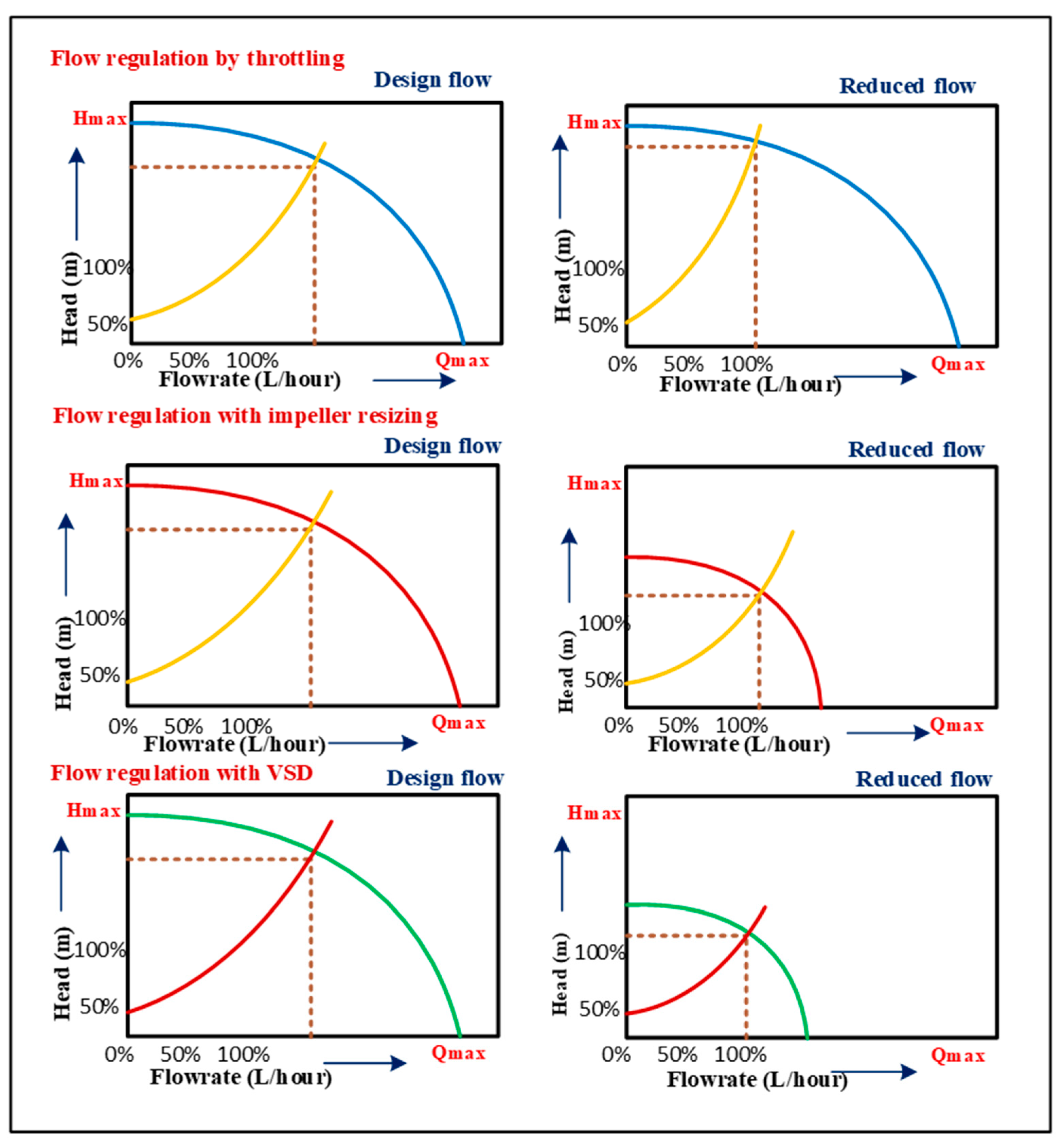
4.1.1. Effects of Different Flow Regulation Strategies on Energy Consumption

The total head (H) as an operation of the flow rate (Q) determines this operation of a centrifugal pump. The total head at the rated speed (Nr) may be easily approximated using the Hr (Qr) functioning feature, which looks like an upward curve, from the pump industrialist’s datasheet. Whenever the pump is running at its most efficient, the optimum pump efficiency point may be attained (BEP). Pumps are harmed when they operate outside of their optimum efficiency region (BER). The above graph it showing the different flow regulation strategies for energy consumption, and it is classified into flow regulation by throttling, flow regulation with impeller resizing, and flow regulation with variable speed drives. So, according to these strategies, the graphs are classified into design flow curves and reduced flow.

4.1.2. Optimizing Pumping Using Variable Speed Drives

Generally, the design responsibility incorporates a number of possibilities to guarantee that a pump with adequate capacity for the pump station’s design life is chosen. Forecasted connection growth, seasonal demand changes, and perhaps firefighting capacity are all examples of contingencies. This demand will not be necessary for the bulk of the pump’s life; therefore, it may be switched off or slowed down if a VSD is added. The use of VSDs is becoming more widespread. The cost of a VSD has dropped so dramatically in recent years that the energy savings might pay the cost of the device in as little as a year. Regrettably, they also make it possible for pumps to be used outside of their intended range. A useful engineering tool may be created using the provided equations and a reasonable amount of time spent getting them to operate. When evaluating the findings, keep in mind that they should only be used as a guide to the pump’s performance at the specified duty. Through operational modifications, however, it is possible to cut energy usage and enhance pump life by analyzing pump performance across a variety of flow rates [37].

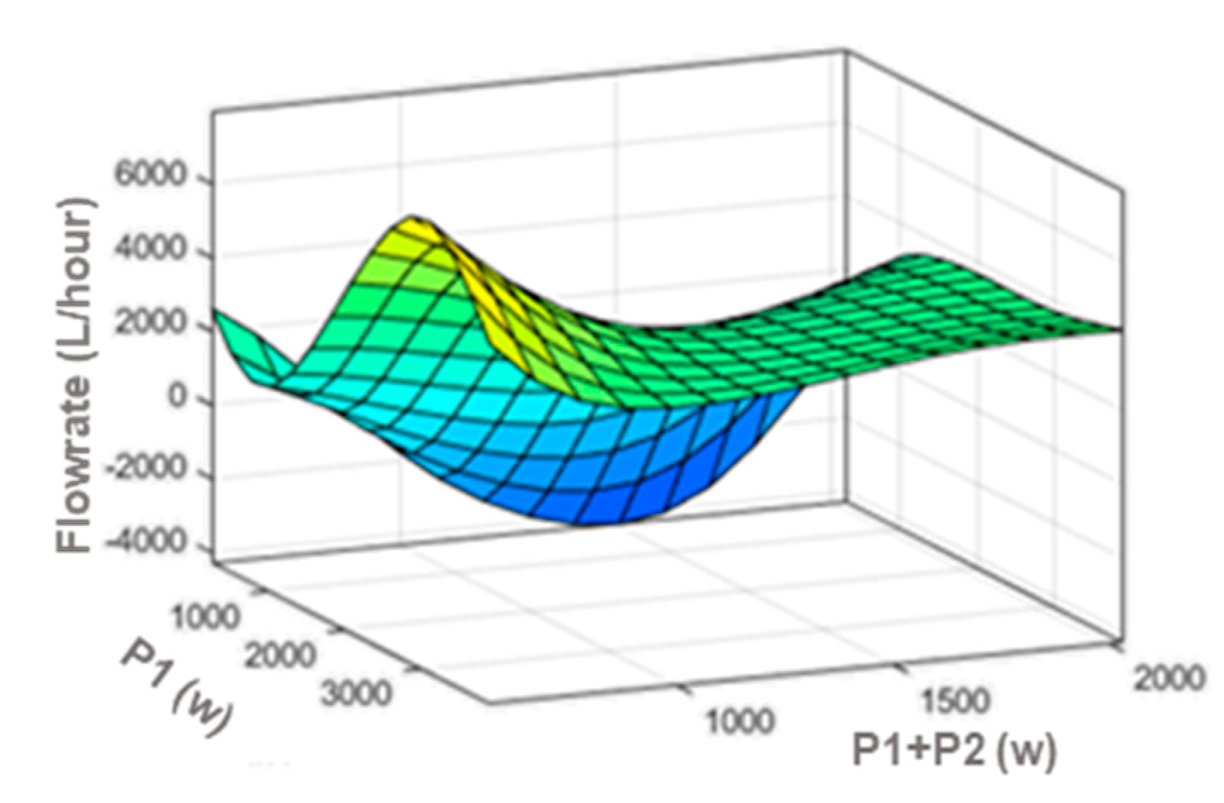
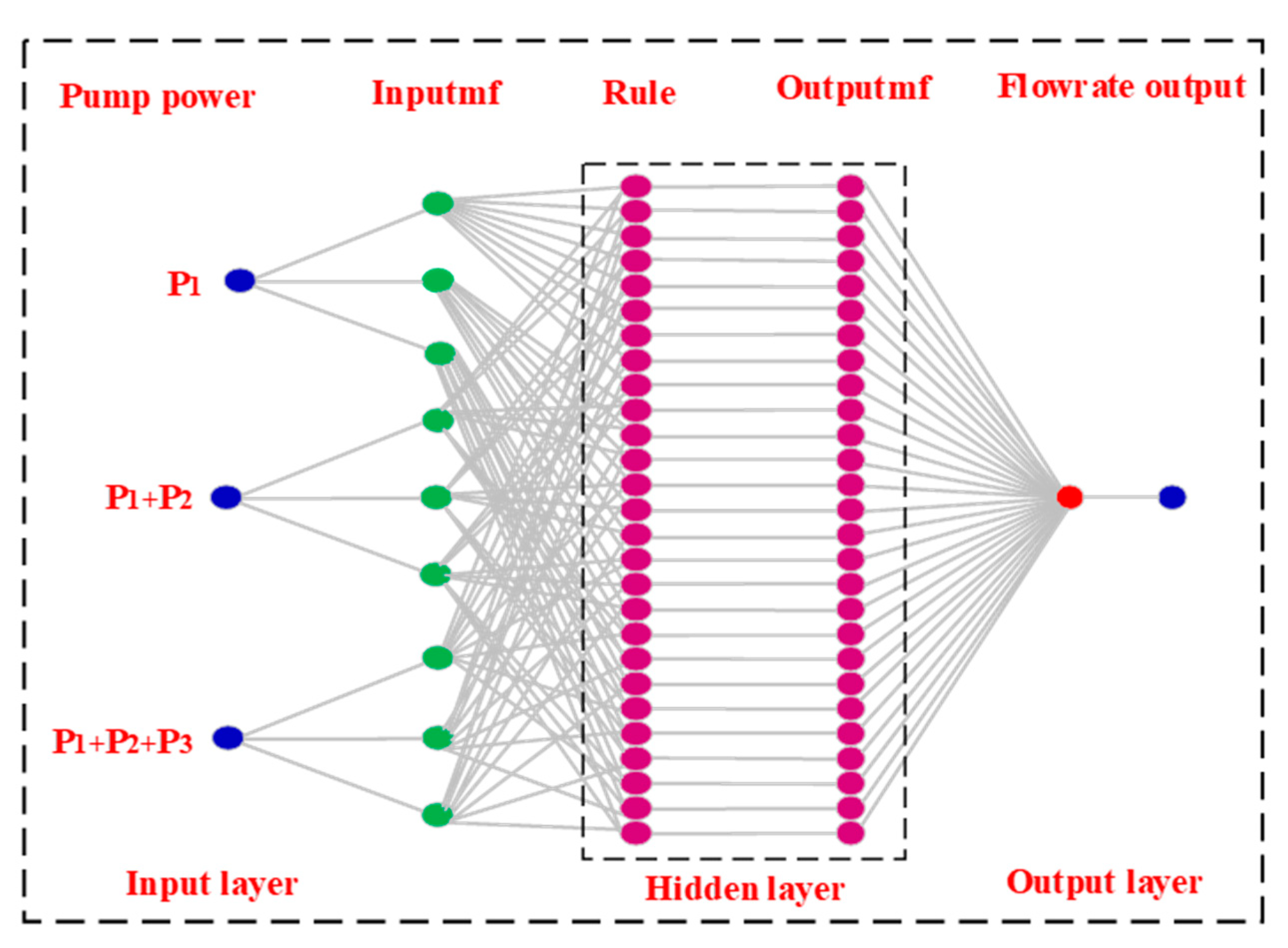
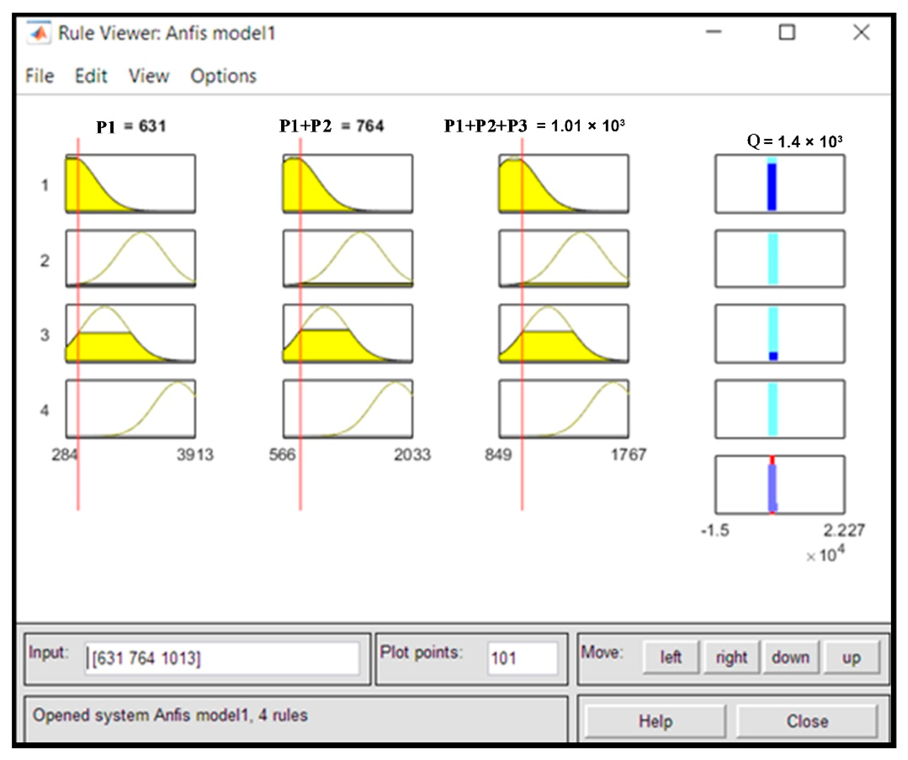
4.1.3. Adaptive Neuro-Fuzzy Inference System

In the anfis architecture, an ANN fuzzy system is combined. This strategy is used to develop a model based on the findings of the experiments. The membership functions are generated using an artificial neural network once the system is characterized using a fuzzy approach. Figure 8 shows the Anfis model structure. The fuzzy layer, product layer, normalized layer, defuzzification layer, and output layer are the five layers that remain used toward training the parameters.
The fuzzy logic program employs a backpropagation technique, either alone or in a mixture by a least-squares approach, to train a fuzzy system using Anfis. In the membership function, the framework of an FIS is tuned throughout this training phase so that the system can represent the input/output data. Figure 9 shows the Anfis surface modeling.
Figure 10 shows the anfis model structure for the defined rule, and the first three columns are the input parameters of the power consumption for each pump, and the fourth column represents the output of the flowrate. The neuro-fuzzy model had five different adaptive layers in its construction. Anfis is a basic data knowledge approach that uses fuzzy logic to transform given inputs into desired outputs, employing broadly coupled neural network compute nodes with weighted data links to convert mathematical inputs into outputs. Anfis integrates the advantages of both machine learning approaches into individual approaches. Anfis operates through tuning the parameters of a FIS using neural network learning methods. Figure 11 depicts the anfis rule creation for the proposed system [38].
In ANFIS, an epoch is the number of iterations. The number of epochs necessary to achieve a specific error tolerance depends on the system and the quantity of data sets. Increase the number of epochs if the error continues to drop at a quicker rate. If the error is progressively decreasing, gradually increase the number of epochs until the error remains constant. More epochs equal more time to train, so keep an eye on the error; if it stays constant, it may cease training and continue to test. It can train the FIS once they have loaded the training data and created the basic FIS structure. To accomplish so, enter the following values in the Train FIS area of Neuro-Fuzzy Designer.
Method of optimization. Choose the hybrid technique for this example, which tunes the FIS parameters using a mix of backpropagation and least-squares regression. The number of training epochs specifies epochs in this case. Error tolerance is a situation that prevents a process from continuing. In this case, a value of 0 implies that the training will end once the number of training epochs has been reached.
For each training epoch, the app shows the training error (as stars) and checking error (as dots). Up to a particular point in the training, the checking error drops, then rises. This rise occurs when the training data becomes overfit. The trained ANFIS model is chosen by the app from the FIS associated with this overfitting point. Trained FIS validates the model with a testing or checking data set that varies from the training data after the FIS has been trained. Use the checking data that has already been loaded for this example. Select Checking data from the Test FIS section to run the FIS against the checking data. Then select Test Now from the drop-down menu. The app displays the testing data set output values (in blue +’s) as well as the output of the trained FIS for the same testing data input values (in red *’s). The FIS output numbers match the predicted result accurately.

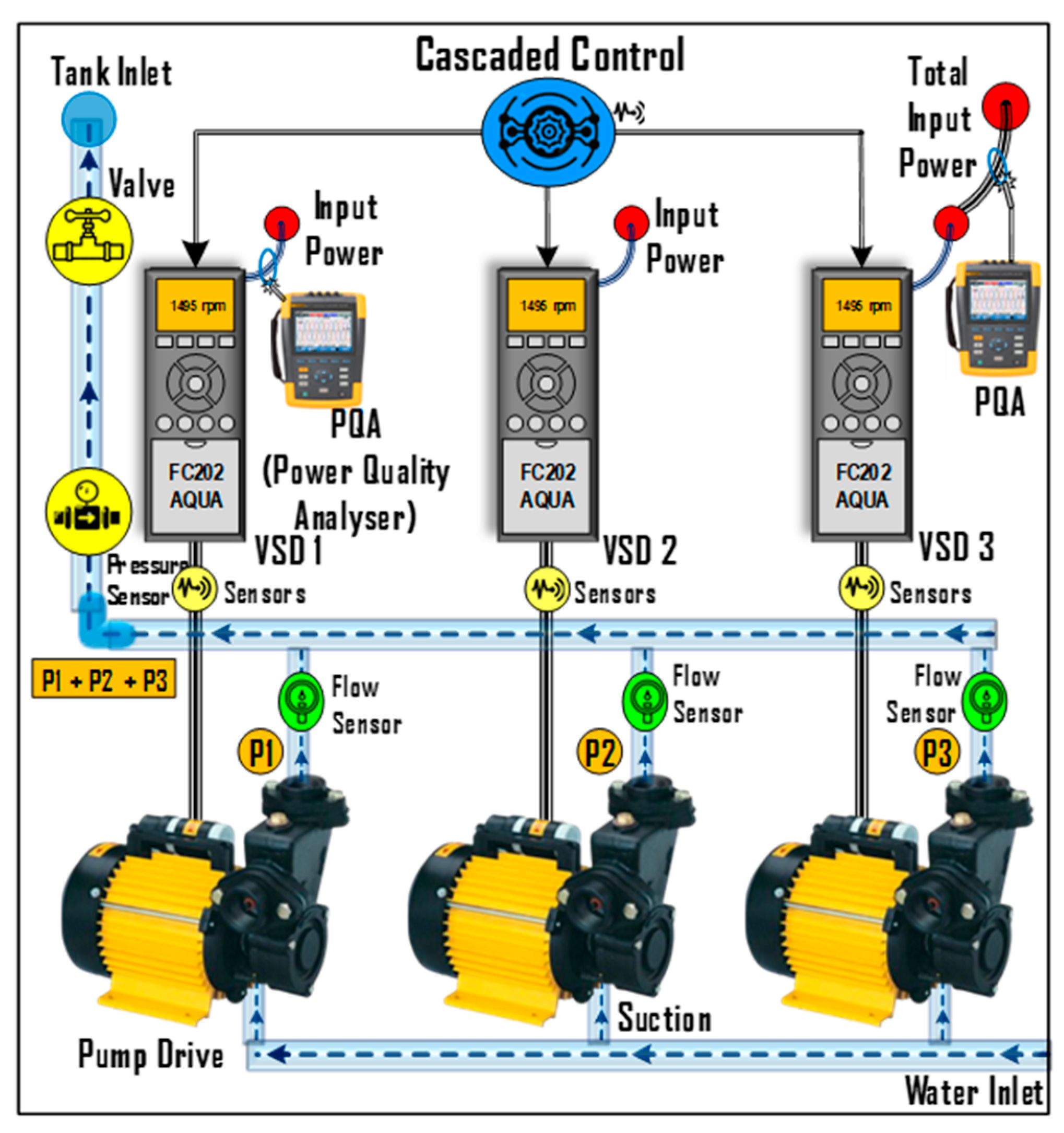
4.2. Experimental Test for Multi-Parallel Pumping System

It is the highest pressure a pump will produce by an assumed speed while the flow rate varies [39]. Table 2 indicates the set point of the cascade pump control w.r.t to flowrate the performance curve for an assumed speed. The pump industrialist similarly gives efficacy and power drawn at several flow rates. The resistance caused by pipes, bends, and valves in a pumping arrangement is shown using a system curve that encompasses both static and frictional inefficiencies. In a closed hydraulic system, only the frictional head is available, but in an open hydraulic system, both static and frictional heads are available. When the pump execution curve and the system curve intersect, the known pumping system is an operational point. Pump 1, on the other hand, begins at the slowest speed possible and increases slightly to the pressure set point [17,18,19].
The investigational arrangement is shown in Figure 12. It contains a 0.55 kW/0.75 hp squirrel cage induction motor (SCIM) also coupled with 2 bar-rated centrifugal inline pumps. Table 3 shows the overall ratings of all the machines.

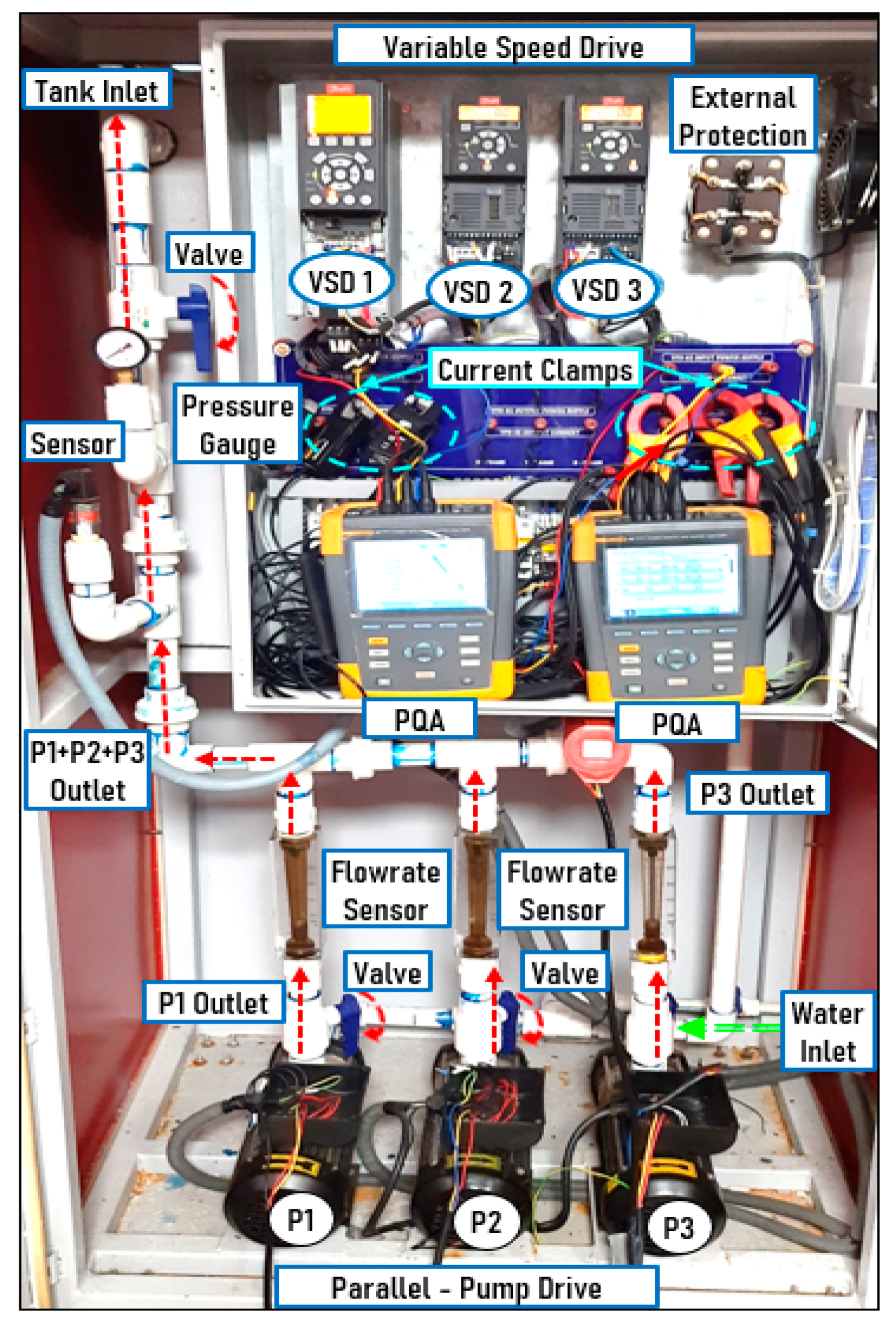
Hardware System Description

Figure 12 shows the experimental setup for the analysis, which consists of three pumps controlled by VSD and relays. The aqua parallel pumping system is powered by a 3-Φ power supply with a frequency of 50 Hz and 415 volts. VSD 1 connects the primary motor–pump unit, which is referred to as pump 1. The second motor is coupled to pump 2 and is connected to VSD 2. The third motor is coupled to pump 3 and is connected to VSD 3. For measuring purposes, a power quality analyzer (PQA) is attached to the drive. In addition, each pump has its own control valve with a flow rate sensor, while the pressure gauge will be linked to the outlet delivery and will be shared by all pumps. To measure the input power, two different types of current clamps will be attached. The VSD 1 is linked to one, and the entire input power of the drive is connected to the other [40].
Inside, the controller logic gate codes are built. Based on that command, the controller is running. The PID controller technique was also incorporated. Based on those logic codes, the sensor data will be transmitted to the controller. A pressure sensor converts pressure into an electrical signal, which comprises metal foil strain gauges mounted onto a diaphragm. As pressure changes, the diaphragm changes shape, causing the resistance in the strain gauges to change, allowing the pressure changes to be measured electrically. Our pressure sensors naturally produce an electrical signal in millivolts that varies proportionally with the pressure and the sensor excitation voltage (mV/V—millivolt per volt).
The frequency converter receives a feedback signal from a sensor in the system. It compares this feedback to a setpoint reference value and determines the error, if any, between these two signals. It then adjusts the speed of the motor to correct this error. The desired static pressure setpoint is the reference signal to the frequency converter. A static pressure sensor measures the actual static pressure in the pipe and provides this information to the frequency converter as a feedback signal. If the feedback signal is greater than the setpoint reference, the frequency converter slows to reduce the pressure. In a similar way, if the pipe pressure is lower than the setpoint reference, the frequency converter speeds up to increase the pressure provided by the pump. While the default values for the frequency converter in a closed loop often provide satisfactory performance, system control can often be optimized by tuning the PID parameters. Auto-tuning is provided for this optimization.
Estimates were made at the point of common coupling (PCC) with a PQ measuring instrument to analyze and record the PQ standards of a cascade pumping arrangement (FLUKE 438). The FLUKE 438 is a class-A instrument that can monitor, record, and calculate three-phase power values [41]. Fluke view software is used to analyze the recorded data. The experiment is carried out with the valve open and the pressure control values ranging from 0.1 to 2 bar. At nominal room temperature, whole PQ measurements were performed on the experimental arrangement. Table 2 shows the experimental configuration that was tested and its design specifications.
Pumping systems use pumps, motors, and variable frequency drives to convert electrical energy to hydraulic energy. Table 3 indicates the specification of the experimental setup.
In addition, when centrifugal pumps are run at lower speeds, affinity laws in pumps be dependable for large energy savings. Compared to a single pumping unit, parallel-coupled centrifugal pumps have a wider operational flow range. The archetype of three pumps is linked in parallel, with Figure 10 showing an archetype of three pumps related in parallel, each through its own suction to the reservoir and then a single transfer section. The parallel associated pumps deliver the sum of separate pump flow rates as well as the pumps’ least common head. The pump head fluctuates with changes in working speed, and system parameters such as piping inner roughness, valves, and bends; also, Table 4 indicates the efficiency and power factor of the pump motor setup [42]. The operating point of a parallel connected pump is determined by the junction of pump execution and system head curve. Individual pumps’ contributions to the total flow rate are determined using their associated pump performance curves. Pumps are often chosen depending on system demand so that they continue to run at their rated flow rate. Operating pumps at less than their rated flow rate lowers efficacy, raises vibration, and shortens pump life.

5. Result and Discussion

Simulation and experiments are carried out on a 0.55 kW SCIM laboratory prototype to test the applicability of the suggested effective utilization approach.

5.1. Simulation Result

Figure 13 represents the graphical presentation of flowrate vs. head with respect to the system curve. By considering set point 1 is 1703 lph the individual motor performs the power rating is 842 W, but if the flow rate increases, the requirement of power is also increasing, and it leads to enhancing the cost as well as reducing the motor life [43]. The initial stage without a load also consumes motor running power. In addition, Figure 14 shows the simulation result of the flow rate vs. power for single and multi-parallel power curves.
To avoid that, coupling of the motor is insisted and compensates for the power even though the flow rate is increased. The above simulation graph clearly illustrated that coupled motor consumes less power than the individual motor pump operation based on the limit setpoint 1 and setpoint 2 values. The first motor–pump unit is referred to as pump 1, which is coupled by VFD. An AC power supply delivering 415 volts at 50 Hz powers the cascade parallel pumping system. This cascade pumping system must be analyzed and recorded; a power quality instrument was used to collect measurements at the point of common coupling. The PQA, fluke-438, is a class-A device capable of recording and monitoring the performance of the pump. The research is carried out by changing the flow rate and speed for our requirements and measurements on the experimental setup [20]. The lowest total power usage of the AC induction motor with multistage pump load. In the simulation, power consumption is reduced, and experimental results were also verified with low power consumed results for all three parallel pumps.

5.2. Experimental Result

Figure 15 shows the adopted experimental result for the power curve for the (a) single pump curve (b), two pump curve, and (c) three pump curve to analyze the performance of power consumption of the AC induction motor with multistage pump load.
Both results for simulation and hardware are mainly used for reducing the energy consumption of the multi-parallel pumping system. For a single pump, the experimental arrangement consists of Figure 15a, which shows the single pump power consumption for the full load condition. It consumes the power of 1650 W for an AC induction motor rating 0.55 kW with a pump load. In two pumps, the experimental arrangement consists of Figure 15b, which shows the pump power is the consumption for an AC induction motor with pump load; also, two pump power is 817 W consumed for an AC induction motor with a rating of 0.55 kW with pump load. It has less power consumption compared to the single pump power. For three pumps, the experimental arrangement consists of Figure 15c, which shows the pump power consumption for an AC induction motor with pump load; also, three pump power is 673 W consumed for an AC induction motor with a rating of 0.55 kW with pump load. It is less power consumption than the previous condition.
In the simulation, by considering set point 1 is 1703 lph, the individual motor performs the power rating is 842 W, but if the flow rate increases, the requirement of power is also increasing, and it leads to enhancing the cost as well as reducing the motor life. To avoid that, coupling of the motor is insisted and compensates for the power even though the flow rate is increased. The above simulation graph clearly illustrated that coupled motor consumes less power than the individual motor pump operation based on the limit setpoint 1 and setpoint 2 values. Table 5 represents the comparison of the energy consumption rate in percentage for modeling and experimental setup.

6. Conclusions

The optimum switching technique for variable speed pumping stations with identical parallel pumps was addressed in this research, which resulted in the lowest total power usage. For a changing total flow, the best switching technique is provided. So, the optimal control system is designed in such a way as to decrease overall losses in the pump system and implement the Anfis for an optimization. The effectiveness of the proposed method is investigated on a real scale of a multi-parallel pump drive system in a Matlab Simulink environment, and investigational validation is accomplished in a laboratory prototype. Experimental verification for expressions that the power saving is based on the setpoint flow rate values. In addition, the comparison of energy consumption rate is given in percentage based on the flowrate values for both modeling and experimental studies.

Author Contributions

All authors contributed equality in each task towards the paper. More specifically: M.B.: Investigation, Software, Validation, Data curation, Formal analysis. R.R.S.: Conceptualization, Methodology, Visualization, Writing, review and editing. All authors have read and agreed to the published version of the manuscript.

Funding

Funded by Vellore Institute of Technology, Vellore, India.

Institutional Review Board Statement

Not applicable.

Informed Consent Statement

Not applicable.

Data Availability Statement

Not applicable.

Conflicts of Interest

The authors declare no conflict of interest.

Nomenclature

ANFISAdaptive neuro-fuzzy inference system
ANNArtificial neural network
AIArtificial intelligence
AEFAArtificial electric field algorithm
BEPBest efficiency point
BERBest efficiency region
CPCentrifugal pump
EPANETEnvironmental Protection Agency Network
FISFuzzy inference system
GAGenetic algorithm
GRNNGeneral regression neural network
HTotal head
IMInduction motor
JMoment of inertia
MINLPMixed-integer nonlinear programming
MFMembership function
NRotational speed
NrRated speed
NNNeural network
NPSHRNet positive suction head
P Number of pole pairs
P1Pump 1
P2Pump 2
P3Pump 3
PCCPoint of common coupling
PQPower quality
PbPump base water level
PATPosition of turbine
PIDProportional integral derivative
PSO-AIWAParticle swarm optimization-adaptive inertia weight adjusting
PQAPower quality analyzer
QFlowrate
SCIMSquirrel cage induction motor
VSDVariable speed drive
VFDVariable frequency drive
V/FVoltage/frequency
VVC+Voltage vector control
WNNWavelet neural network
A(Y)Nonlinear function
MPPassive/resistive torque of the pump
MζViscous torque
MMTActive torque from the asynchronous motor
fNetwork frequency
qv1Input flow
TLLoad torque
qv2Output water flow
ωAngular velocity
kvValve constant
N0Nominal speed
Qp2, Qp3Flow ranges
p2Pressure valve 2
Rm, XmDissipative and reactive hydro-resistances
RΔH, XΔHLosses of hydraulic head in CP’s spiral venting
RΔQ, XΔQFeedback on the CP’s head through the seal
XtReactive hydro-resistance of the spiral part of the CP’s venting
XμH, XμQFinite number of the impeller’s blades on the pump’s pressure and volumetric fluid losses
H1 = (H1d + jH1q)Phasor of rated head of ideal pump in non-functional mode
Q1, Q2, QmPhasors of rated volumetric fluid losses of ideal CP
H2(Q2)Static head characteristics of hydraulic network
Hcpn, Qcpn Nominal head and volumetric loss of fluid in CP
Scpn, ZcpnNominal power and module of hydraulic impedance of CP;
ρ Per unit density of fluid
gGravitational constant
H2 = (H2d + jH2q)Phasor of hydraulic network head
H1nNominal head of idealized CP in no-load mode
Q 2 = Q 2 d 2 + Q 2 q 2 Actual volumetric losses
H 2 = H 2 d 2 + H 2 q 2 Actual head of real CP
Rg2(Q2d, Q2q) = H2 (Q2)/Q2Hydraulic resistance of hydraulic network
NcpMechanical power on the Shaft of CP
N2Hydraulic power on the output of CP
ωbBase angular velocity
ω r Rotor angular speed
r s , r r Stator and rotor resistance
L M Mutual inductance
ψ ds , ψ qs Stator flux of d-axis and q-axis
ψ dr , ψ qr Rotor flux of d-axis and q-axis
λ abcs , λ abcr Flux linkages of stator and rotor
PpumpinPump input power
RSStator resistance
RrRotor resistance
X1 and X2Stator and rotor leakage reactance
XhMain reactance
RfeIron loss resistance
kOperative stator/rotor turns ratio
μ(x) and μ(y)Gaussian membership functions
ciFuzzy set breadth
σiTraining cost
wiNormalized firing strength
pi, qi, and riSubsequent parameters for network’s training phase
S1 and S2Slip

References

  1. Li, W.; Vaziri, V.; Aphale, S.S.; Dong, S.; Wiercigroch, M. Energy saving by reducing motor rating of sucker-rod pump systems. Energy 2021, 228, 120618. [Google Scholar] [CrossRef]
  2. de Souza, D.F.; da Guarda, E.L.A.; Sauer, I.L.; Tatizawa, H. Energy Efficiency Indicators for Water Pumping Systems in Multifamily Buildings. Energies 2021, 14, 7152. [Google Scholar] [CrossRef]
  3. Waide, P.; Brunner, C.U. Energy-Efficiency Policy Opportunities for Electric Motor-Driven Systems; IEA Energy Papers; OECD Publishing: Paris, France, 2011; pp. 1–132. [Google Scholar] [CrossRef]
  4. Wang, Y.; Wang, Z.; Wang, Z. A stochastic load demand-oriented synergetic optimal control strategy for variable-speed pumps in residential district heating or cooling systems. Energy Build. 2021, 238, 110853. [Google Scholar] [CrossRef]
  5. Wilson, A. The pump industry—past, present and future. World Pumps 2016, 2016, 36–38. [Google Scholar] [CrossRef]
  6. Ahn, K.U.; Park, S.H.; Hwang, S.; Choi, S.; Park, C.S. Optimal control strategies of eight parallel heat pumps using Gaussian process emulator. J. Build. Perform. Simul. 2019, 12, 650–662. [Google Scholar] [CrossRef]
  7. Zhao, H.; Wang, Y.; Chen, G.; Zhan, Y.; Xu, G. Precise Determination of Power-Off Time of Intermittent Supply Technology Based on Fuzzy Control for Energy Saving of Beam Pumping Motor Systems. Electr. Power Components Syst. 2018, 46, 197–207. [Google Scholar] [CrossRef]
  8. Nikolenko, I.V.; Ryzhakov, A.N. Parallel operation mode optimization of different-type centrifugal pumps of a water supply booster pumping station. In Proceedings of the 2020 International Conference on Dynamics and Vibroacoustics of Machines (DVM), Samara, Russia, 16–18 September 2020. [Google Scholar] [CrossRef]
  9. Izquierdo, M.D.Z.; Jimenez, J.J.S.; Del Sol, A.M. Matlab software to determine the saving in parallel pumps optimal operation systems, by using variable speed. In Proceedings of the 2008 IEEE Energy 2030 Conference, Atlanta, GA, USA, 17–18 November 2008; Volume 2. [Google Scholar] [CrossRef]
  10. Wang, X.; Zhao, Q.; Wang, Y. An asynchronous distributed optimization method for energy saving of parallel-connected pumps in HVAC systems. Results Control Optim. 2020, 1, 100001. [Google Scholar] [CrossRef]
  11. Gruys, E. Bildbericht Nr. Magentorsion bei einem Schwein. Dtsch. Tierarztl. Wochenschr. 1974, 81, 411. [Google Scholar]
  12. Islam, A.; Singh, J.G.; Jahan, I.; Lipu, M.S.H.; Jamal, T.; Elavarasan, R.M.; Mihet-Popa, L. Modeling and Performance Evaluation of ANFIS Controller-Based Bidirectional Power Management Scheme in Plug-In Electric Vehicles Integrated With Electric Grid. IEEE Access 2021, 9, 166762–166780. [Google Scholar] [CrossRef]
  13. De Wrachien, D.; Mambretti, S.; Orsi, E.; Brebbia, C.A.; Ursino, N. Optimization of pump operations in a complex water supply network: New genetic algorithm frameworks. Int. J. Sustain. Dev. Plan. 2017, 12, 79–88. [Google Scholar] [CrossRef]
  14. Ekster, A. Optimization of Pump Station Operation Saves Energy and Reduces Carbon Footprint. Proc. Water Environ. Fed. 2009, 2009, 3762–3770. [Google Scholar] [CrossRef]
  15. Wu, P.; Lai, Z.; Wu, D.; Wang, L. Optimization Research of Parallel Pump System for Improving Energy Efficiency. J. Water Resour. Plan. Manag. 2015, 141, 04014094. [Google Scholar] [CrossRef]
  16. Moazeni, F.; Khazaei, J. Optimal energy management of water-energy networks via optimal placement of pumps-as-turbines and demand response through water storage tanks. Appl. Energy 2020, 283, 116335. [Google Scholar] [CrossRef]
  17. Sarmas, E.; Spiliotis, E.; Marinakis, V.; Tzanes, G.; Kaldellis, J.K.; Doukas, H. ML-based energy management of water pumping systems for the application of peak shaving in small-scale islands. Sustain. Cities Soc. 2022, 82, 103873. [Google Scholar] [CrossRef]
  18. Luna, T.; Ribau, J.; Figueiredo, D.; Alves, R. Improving energy efficiency in water supply systems with pump scheduling optimization. J. Clean. Prod. 2019, 213, 342–356. [Google Scholar] [CrossRef]
  19. Hieninger, T.; Schmidt-Vollus, R.; Schlücker, E. Improving energy efficiency of individual centrifugal pump systems using model-free and on-line optimization methods. Appl. Energy 2021, 304, 117311. [Google Scholar] [CrossRef]
  20. Hieninger, T.; Goppelt, F.; Schmidt-Vollus, R.; Schlücker, E. Energy-saving potential for centrifugal pump storage operation using optimized control schemes. Energy Effic. 2021, 14, 23. [Google Scholar] [CrossRef]
  21. Ping, X.; Yao, B.; Niu, K.; Yuan, M. A Machine Learning Framework With an Intelligent Algorithm for Predicting the Isentropic Efficiency of a Hydraulic Diaphragm Metering Pump in the Organic Rankine Cycle System. Front. Energy Res. 2022, 10, 1–14. [Google Scholar] [CrossRef]
  22. Feng, X.; Qiu, B.; Wang, Y. Optimizing Parallel Pumping Station Operations in an Open-Channel Water Transfer System Using an Efficient Hybrid Algorithm. Energies 2020, 13, 4626. [Google Scholar] [CrossRef]
  23. Wang, X.; Zhao, Q.; Wang, Y. A Distributed Optimization Method for Energy Saving of Parallel-Connected Pumps in HVAC Systems. Energies 2020, 13, 3927. [Google Scholar] [CrossRef]
  24. Gu, X.; Li, T.; Liao, Z.; Yang, L.; Nie, L. Modeling and Optimization of Beam Pumping System Based on Intelligent Computing for Energy Saving. J. Appl. Math. 2014, 2014, 317130. [Google Scholar] [CrossRef] [Green Version]
  25. Abdelsalam, A.A.; Gabbar, H.A. Energy Saving and Management of Water Pumping Networks. Heliyon 2021, 7, e07820. [Google Scholar] [CrossRef] [PubMed]
  26. Sharabiani, V.R.; Kaveh, M.; Taghinezhad, E.; Abbaszadeh, R.; Khalife, E.; Szymanek, M.; Dziwulska-Hunek, A. Application of Artificial Neural Networks, Support Vector, Adaptive Neuro-Fuzzy Inference Systems for the Moisture Ratio of Parboiled Hulls. Appl. Sci. 2022, 12, 1771. [Google Scholar] [CrossRef]
  27. Cao, Y.; Mohammadzadeh, A.; Tavoosi, J.; Mobayen, S.; Safdar, R.; Fekih, A. A new predictive energy management system: Deep learned type-2 fuzzy system based on singular value decommission. Energy Rep. 2021, 8, 722–734. [Google Scholar] [CrossRef]
  28. Enayatollahi, H.; Sapin, P.; Unamba, C.; Fussey, P.; Markides, C.; Nguyen, B. A Control-Oriented ANFIS Model of Evaporator in a 1-kWe Organic Rankine Cycle Prototype. Electronics 2021, 10, 1535. [Google Scholar] [CrossRef]
  29. Subramaniam, U.; Elavarasan, R.M.; Raju, K.; Shanmugam, P. Sensorless parameter estimation of VFD based cascade centrifugal pumping system using automatic pump curve adaption method. Energy Rep. 2021, 7, 453–466. [Google Scholar] [CrossRef]
  30. Briceño-León, C.; Iglesias-Rey, P.; Martinez-Solano, F.; Mora-Melia, D.; Fuertes-Miquel, V. Use of Fixed and Variable Speed Pumps in Water Distribution Networks with Different Control Strategies. Water 2021, 13, 479. [Google Scholar] [CrossRef]
  31. Olszewski, P. Genetic optimization and experimental verification of complex parallel pumping station with centrifugal pumps. Appl. Energy 2016, 178, 527–539. [Google Scholar] [CrossRef]
  32. Hieninger, T.; Goppelt, F.; Schmidt-Vollus, R. On-line self-tuning for centrifugal pumps driven in parallel mode using dynamic optimization. In Proceedings of the 2018 18th International Conference on Mechatronics—Mechatronika (ME), Brno, Czech Republic, 5–7 December 2018. [Google Scholar]
  33. Van Erp, R.; Kampitsis, G.; Matioli, E. Efficient Microchannel Cooling of Multiple Power Devices With Compact Flow Distribution for High Power-Density Converters. IEEE Trans. Power Electron. 2019, 35, 7235–7245. [Google Scholar] [CrossRef]
  34. Ekta; Garg, V.K. Advance lighting and water pumping system using artificial intelligence. In Proceedings of the 2018 Fifth International Conference on Parallel, Distributed and Grid Computing (PDGC), Solan, India, 20–22 December 2018; pp. 669–675. [Google Scholar] [CrossRef]
  35. Viholainen, J.; Tamminen, J.; Ahonen, T.; Ahola, J.; Vakkilainen, E.; Soukka, R. Energy-efficient control strategy for variable speed-driven parallel pumping systems. Energy Effic. 2012, 6, 495–509. [Google Scholar] [CrossRef]
  36. Pechenik, M.; Burian, S.; Pushkar, M.; Zemlianukhina, H. Analysis of the Energy Efficiency of Pressure Stabilization Cascade Pump System. In Proceedings of the 2019 IEEE International Conference on Modern Electrical and Energy Systems (MEES), Kremenchuk, Ukraine, 23–25 September 2019; pp. 490–493. [Google Scholar] [CrossRef]
  37. Engineer, O.; Water, F.R. Optimising pumping using variable speed drives. Future Boost. Pump Technol. 2017, 2017, 1–6. [Google Scholar]
  38. Xu, Y.; Guo, Z.; Yuan, C. Feasibility study of an integrated air source heat pump water heater/chillers and exhaust gas boiler heating system for swimming pool on luxury cruise ship. Energy Rep. 2021, 8, 1260–1282. [Google Scholar] [CrossRef]
  39. Lai, Z.; Li, Q.; Zhao, A.; Zhou, W.; Xu, H.; Wu, D. Improving Reliability of Pumps in Parallel Pump Systems Using Particle Swam Optimization Approach. IEEE Access 2020, 8, 58427–58434. [Google Scholar] [CrossRef]
  40. Zou, T.-H.; Ma, S.-Y. Analysis on energy saving of pumps movement adjustment in a closed cycle. In Proceedings of the 2010 Asia-Pacific Power and Energy Engineering Conference, Chengdu, China, 28–31 March 2010; pp. 1–4. [Google Scholar] [CrossRef]
  41. Shankar, V.A.; Subramaniyan, U.; Sanjeevikumar, P.; Holm-Nielsen, J.B.; Blaabjerg, F.; Paramasivam, S. Experimental Investigation of Power Signatures for Cavitation and Water Hammer in an Industrial Parallel Pumping System. Energies 2019, 12, 1351. [Google Scholar] [CrossRef] [Green Version]
  42. Fan, X.; Sun, H.; Yuan, Z.; Li, Z.; Shi, R.; Razmjooy, N. Multi-objective optimization for the proper selection of the best heat pump technology in a fuel cell-heat pump micro-CHP system. Energy Rep. 2020, 6, 325–335. [Google Scholar] [CrossRef]
  43. Arun Shankar, V.K.; Umashankar, U.; Paramasivam, S.; Hanigovszki, N. An Energy Efficient Control Algorithm for Parallel Pumping Industrial Motor Drives System. In Proceedings of the 2018 IEEE International Conference on Power Electronics, Drives and Energy Systems (PEDES), Chennai, India, 18–21 December 2018. [Google Scholar] [CrossRef]
Figure 1. Equivalent circuit of centrifugal pump.
Energies 15 04343 g001
Figure 2. Simplified induction motor equivalent circuit.
Energies 15 04343 g002
Figure 3. ANFIS architecture.
Energies 15 04343 g003
Figure 4. Various flow regulation strategies on energy consumption (Reprinted from: www.iipinetwork.org. Accessed from 29 January 2022).
Energies 15 04343 g004
Figure 5. Parallel pump system.
Energies 15 04343 g005
Figure 6. Parallel pump operation.
Energies 15 04343 g006
Figure 7. Parallel pump operational curve.
Energies 15 04343 g007
Figure 8. Simulation model of the pumping structure.
Energies 15 04343 g008
Figure 9. Anfis surface output.
Energies 15 04343 g009
Figure 10. ANFIS model structure.
Energies 15 04343 g010
Figure 11. Anfis rule creation.
Energies 15 04343 g011
Figure 12. Single and multi-parallel experimental setup.
Energies 15 04343 g012
Figure 13. Pump curve vs. system curve.
Energies 15 04343 g013
Figure 14. Single and multi-parallel power curve.
Energies 15 04343 g014
Figure 15. Power curve of (a) single pump curve, (b) two pump curve (c), three pump curve.
Energies 15 04343 g015
Table 1. Different types of pump optimization algorithms with application.
Algorithm TypeOperationApplication
Genetic algorithm [13]Significant progress has been made in the transition from a discrete to a continuous description of pump operation.The procedure is random. Various situations with virtually comparable energy usage.
Pump stations optimization [14] The established optimized schedule resulted in a 16KW*HR/MG energy reduction, which is over 25%.Only fixed-speed motors were subjected to optimization.
Manufacturer’s curves were used instead of actual performance curves.
The developed optimization model employs a genetic algorithm (GA) [15]The GA and Lagrange multiples techniques were used to show a simple theoretical solution for optimizing the functioning of two identical pumps.Recommending the most appropriate operating mode, This optimization model balances between efficiency and dependability.
Two mixed-integer nonlinear programming (MINLP) [16] Determine the best quantity and position of turbine pumps (PATs).Reduce energy generating costs in water-energy systems.
Energy management method [17]The creation of a scheduling system and an ensemble of machine learning models for precisely forecasting RES production and energy usage.Water pumping station operation hours are scheduled.
Reduce the electricity usage.
Hybrid optimization method
(EPANET) [18]
Water demand, and water storage risk, digital technologies may be used to improve the system with little investment in equipment or physical interaction.Enhance the energy efficiency of a water delivery system.
To obtain the sustainable water management system.
Model-free optimization [19]The direct search strategy is typically the best solution for single pump systems.The energy optimum of the single pump system.
Control optimization [20]The impact of various system factors is investigated using twelve centrifugal pumps with nominal powers ranging from 1 to 120 kW.To reduce the operational time, are critical for a cost-effective operation.
Wavelet neural network (WNN) with momentum term and particle swarm optimization-adaptive inertia weight adjusting (PSO-AIWA), [21]When studying the time-varying features of the pump’s essential operational parameters, there are several constraints.The evaluation of efficiency limits and optimum cycle parameters.
Efficient Hybrid Algorithm [22]Parallel pumping station functioning in an open-channel water transfer system.For real-time system optimization, the DA–SA–PSO is quite effective.
Distributed optimal control algorithm [23] The pump optimization issue in a distributed fashion, achieving the lowest possible pump energy usage while ensuring convergence.
Energy savings potential, convergence assurance, and adaptability.
Regression neural network (GRNN) algorithm [24]This approach does not need any modifications to the original equipment; it just attempts to make the device function in an energy-saving mode.The optimal conditions result in a 5.34% oil yield and a 3.75% reduction in electric power usage.
Artificial electric field algorithm [25]It is an iterative process including an optimization algorithm and the
EPANET hydraulic simulator.
Its findings reveal that AEFA is superior in terms of convergence and cost savings.
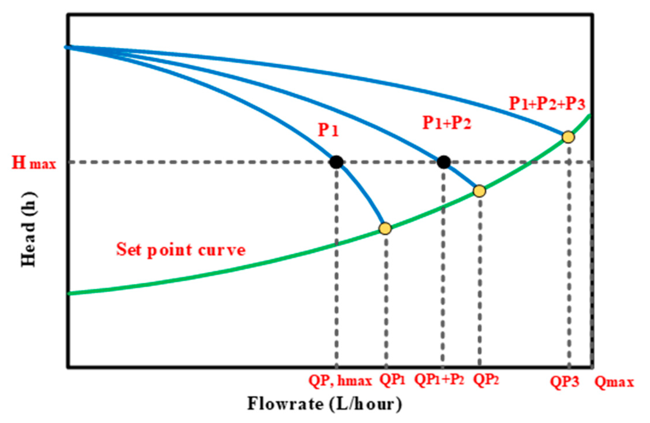
Table 2. Pump setpoint flowrates in cascade pump control.
Setpoint Flowrate (lph)Pump 1Pump 2Pump 3
1 to 1703 lphONOFFOFF
1703 to 3285 lphONONOFF
Above 3285 lphONONON
Table 3. Specification of experimental setup.
ParticularValues
Rated power0.55 kW/0.75 HP
Rated voltage415 V
Frequency50 Hz
Rated current1.7 A
Head23.5 m
Nominal speed2800 rpm
Motor selectionAsynchronous
Configuration modeOpen-loop
Motor control principleV/F
Overload mode Normal torque
Clockwise directionNormal
Pump typeCentrifugal
ISC3.3 A
Head range18/25 m
Discharge2000 (Lph)
Duty typeS1
Pipe size25 × 25 mm
Model PH2-30 CI
INSULCLASS ‘F’
Stator resistance (RS)13.1083 Ohm
Rotor resistance (Rr)11.9789 Ohm
Stator and rotor leakage reactance (X1 and X2)11.3003 Ohm
Main reactance (Xh)212.7426 Ω
Iron loss resistance (Rfe)5182.820 Ω
Number of pole pair2
Simulation typeContinuous (or) discrete
Port configurationTorque
Stator and rotor inductance0.035969972 H
Mutual inductance0.677180727 H
Table 4. Efficiency and power factor for pump motor.
Load1/41/21/3Full
Efficiency (%)72757778
Power factor (%)68707581
Table 5. Comparison of the energy consumption rate in percentage for modeling and experimental setup.
Flowrate (p.u)Power Consumption Rate for Simulation (%)Power Consumption Rate for Experimental Set Up (%)
P1P1 + P2P1 + P2 + P3P1P1 + P2P1 + P2 + P3
0.249.1%72%100%53.2%76.7%100%
0.497.5%84.3%100%95.1%79.2%100%
0.6100%63.7%65.9%100%65%69.2%
0.8100%55.9%52.2%100%57.9%54%
1100%51.9%45.1%100%55%47.4%
Publisher’s Note: MDPI stays neutral with regard to jurisdictional claims in published maps and institutional affiliations.

