Physics-Based Proxy Modeling of CO₂ Sequestration in Deep Saline Aquifers

Abstract

The geological sequestration of CO₂ in deep saline aquifers is one of the most effective strategies to reduce greenhouse emissions from the stationary point sources of CO₂. However, it is a complex task to quantify the storage capacity of an aquifer as it is a function of various geological characteristics and operational decisions. This study applies physics-based proxy modeling by using multiple machine learning (ML) models to predict the CO₂ trapping scenarios in a deep saline aquifer. A compositional reservoir simulator was used to develop a base case proxy model to simulate the CO₂ trapping mechanisms (i.e., residual, solubility, and mineral trapping) for 275 years following a 25-year CO₂ injection period in a deep saline aquifer. An expansive dataset comprising 19,800 data points was generated by varying several key geological and decision parameters to simulate multiple iterations of the base case model. The dataset was used to develop, train, and validate four robust ML models—multilayer perceptron (MLP), random forest (RF), support vector regression (SVR), and extreme gradient boosting (XGB). We analyzed the sequestered CO₂ using the ML models by residual, solubility, and mineral trapping mechanisms. Based on the statistical accuracy results, with a coefficient of determination (R²) value of over 0.999, both RF and XGB had an excellent predictive ability for the cross-validated dataset. The proposed XGB model has the best CO₂ trapping performance prediction with R² values of 0.99988, 0.99968, and 0.99985 for residual trapping, mineralized trapping, and dissolution trapping mechanisms, respectively. Furthermore, a feature importance analysis for the RF algorithm identified reservoir monitoring time as the most critical feature dictating changes in CO₂ trapping performance, while relative permeability hysteresis, permeability, and porosity of the reservoir were some of the key geological parameters. For XGB, however, the importance of uncertain geologic parameters varied based on different trapping mechanisms. The findings from this study show that the physics-based smart proxy models can be used as a robust predictive tool to estimate the sequestration of CO₂ in deep saline aquifers with similar reservoir characteristics.

1. Introduction

The atmospheric concentration of carbon dioxide (CO₂) was recorded as 419.5 parts per million (ppm) in May 2021, representing an approximately 50% increase compared to the beginning of the industrial revolution [1,2]. Carbon dioxide is a greenhouse gas that results in global warming and adverse climatic changes. The recent global efforts to reduce CO₂ emissions have prompted a widespread push towards renewable energy sources to replace fossil fuels and increase fuel conservation/efficiency. Despite these efforts, fossil fuels are still predicted to be the primary energy source for the foreseeable future [3]. Carbon capture and storage (CCS) technology has been proposed to mitigate the effects of climate change. CCS aims to store the emissions from significant stationary sources of CO₂ such as power plants and industries in deep geological formations such as the saline aquifers. Szulczewski et al. [4] reported that the United States has sufficient subsurface capacity to store captured emissions from the power sector for at least 100 years.

The trapping of buoyant CO₂ injected into a reservoir requires the existence of low permeability caprocks that would impede the upward migration and leakage of the injected CO₂. Although depleted oil and gas reservoirs can store CO₂ using the exact mechanism that initially traps oil and gas, deep saline aquifers offer a significantly large storage capacity [5]. Furthermore, suitable aquifers are more widely available all over the world. Thus, CCS is one of the most promising technologies to power the world with fossil fuels while mitigating the adverse effects of CO₂ emissions [6].

About 15 large-scale commercial CCS projects are scattered worldwide, with an annual sequestration of 23 million tons of CO₂ [1]. According to the Global CCS Institute, several pilot/demonstration and commercial CCS projects are underway, mainly in North America, Europe, and China [7]. A viable CCS site has reservoir conditions suitable for the injected CO₂ to exist in a supercritical state. The supercritical CO₂ density ranges between 200–800 kg/m³ in subsurface conditions, significantly higher than the density of gaseous CO₂ (2 kg/m³). Therefore, the supercritical state substantially improves the mass of CO₂ that can be injected into the pores initially saturated with brine.

Several experimental and numerical studies have evaluated the various aspects of CO₂ sequestration in deep saline aquifers. The experimental studies have focused on multiple aspects of CO₂ sequestration in deep saline aquifers, such as dissolution trapping, mineral trapping, residual trapping, and other mechanisms [8,9]. However, the results from the experimental studies are difficult to scale to the basin level and involve several simplifying assumptions to model the actual field conditions [6].

The physics-based numerical and analytical models are the most effective tools for modeling CO₂ sequestration in deep saline aquifers. The numerical models can capture various aspects of CO₂ storage by different mechanisms in deep saline aquifers [10,11,12,13,14,15,16,17]. Pruess et al. [16] presented scoping studies of the amount of CO₂ that could be trapped in gas, aqueous, and solid phases. Their studies showed that a significant amount of CO₂ is sequestered by precipitation as secondary carbonates and aqueous dissolution. Kumar et al. [18] presented the results from a compositional reservoir simulation of a typical sequestration project in a deep saline aquifer to understand and quantify the CO₂ sequestered due to different mechanisms. They varied the other geological parameters in their base case model to show that aqueous and mineral trapping was the most effective CO₂ storage mechanism. However, residual gas trapping was more effective in safe CO₂ sequestration under some situations. Xu et al. [19] numerically studied the sequestration of CO₂ by mineral trapping. They evaluated three different types of aquifer mineral compositions to conclude that CO₂ sequestration by mineralization varies considerably with the rock type. They also observed that the mineralization adversely impacts the porosity and permeability of the reservoir. Birkholzer and Zhou [20] performed a basin-scale simulation on a hypothetical Illinois Basin to show that the estimate of the storage capacity of a reservoir cannot be based solely on the effective pore volume. They concluded that the far-field pressure buildup and its impact on caprock integrity need to be correctly accessed before initiating a CCS project. Bryant et al. [21] evaluated the intrinsic instability of a buoyancy-driven displacement during the injection of CO₂ in deep saline aquifers. Doughty [22] further estimated the CO₂ plume stabilization in a reservoir where 1 million metric tons of CO₂ was injected throughout 4 years. Results from numerical models showed that the CO₂ plume is effectively immobilized at 25 years and is safely sequestered in the presence of a caprock. Hesse [23] presented a compact multiscale finite volume model for the numerical simulation of CO₂ sequestration in large-scale heterogeneous formations. They identified that dissolution is the most crucial trapping mechanism, which is enhanced by the high permeability of the reservoirs. Jiang et al. [24] reviewed various numerical modeling techniques for the long-term sequestration of CO₂. Ahmmed [25] used numerical reservoir simulation to model reservoir behavior caused by the CO₂ injection near an individual well in the Farnsworth Unit in northern Texas, USA. The simulation results showed that hydrodynamic trapping was the primary mechanism of CO₂ sequestration. The mineral trapping was insignificant, with ankerite as the only mineral that sequestered CO₂. Pan et al. [26] and Khan et al. [27] both simulated the alternating water gas (WAG) injection to understand the impact of various minerals present in the aquifer on the reservoir permeability, porosity, and other fluid flow properties. Bao et al. [28] performed a large-scale CO₂ sequestration by coupling a reservoir simulation with a molecular dynamic simulation (MD) on massively parallel high-performance computing systems. Foroozesh et al. [14] conducted a field-scale simulation of CO₂ injections in saline aquifers for ten years. Their results showed that solubility trapping was the primary mechanism of CO₂ sequestration. Numerous other studies have explored different aspects of CO₂ sequestration in deep saline aquifers, including the effect of geology on trapping behavior [29], the trapping efficiency due to various trapping mechanisms, and the risks associated with the leakage of the storage sites [30].

Numerical reservoir simulations are often complex, time consuming, and resource intensive despite their versatility. It takes a long time to process the simulation data for sensitivity analysis and optimization studies. In addition, each additional reservoir simulation requires a large set of complex geological data. Predictive modeling of CO₂ geological storage is crucial for initiating a CCS project and setting standards for storage and regulations. Although a robust and fully validated reservoir simulation model, which requires significant geological data, is necessary when the project is fully mature, often accurate, reliable, and quick results are needed for initial screening and sensitivity studies.

Recently, supervised machine learning has been used to solve several complex problems in science and engineering by creating predictive proxy models to circumvent some drawbacks of complex models during the early part of a project. In addition, machine learning models can identify complex relationships between inputs and outputs, identify patterns, and generate solutions to complex problems. Thus, several studies use supervised machine learning for reservoir characterization, production forecasting, well spacing optimization, monitoring, testing, history matching, fluid property estimation, enhanced oil recovery, outlier detection, etc. [31,32,33,34,35].

Machine learning models have also been used to study CCS operations. For example, Le and Chon [36] used the artificial neural network (ANN) to evaluate the performance of CO₂-EOR by measuring the oil recovery factor, gas–oil ratio, cumulative CO₂ production, and net CO₂ storage. They concluded that the ANN generated an accurate proxy model for various reservoir conditions to optimize oil recovery and the long-term storage of CO₂. Other studies have used different ANN models to optimize the CO₂-EOR projects [37] and estimate the oil recovery performance of depleted reservoirs [38]. Ahmadi et al. [34] used an ANN to predict the feasibility of CO₂ sequestration in CCS in deep saline aquifers. They used 800 different data points from the literature to predict the viscosity of the injected CO₂ by using an ANN. Kim et al. [39] used an ANN for storage efficiency in a saline aquifer. They varied different reservoir properties such as permeability, porosity, thickness, residual oil saturation, and depth to generate 150 other reservoir models used to create the proxy model based on an ANN.

For most studies involving the application of machine learning models for CCS, the CO₂ sequestration due to mineral trapping is not simulated mainly to reduce the computational time. During mineralization, the dissolved CO₂ reacts with the minerals in the rock and cations in the pore water to form stable mineral precipitates. The precipitates permanently trap the carbon, even in the case of caprock leakage and during the plume migration. However, one of the shortcomings of mineral trapping as a CO₂ sequestration mechanism is the prolonged rate of reaction, which may take several hundreds of years to complete [19]. There is also a high degree of uncertainty in the chemical composition of the formation water and rock [19]. Despite being one of the most secure methods to sequester CO₂, there have not been many studies using machine learning methods that include the impact of various minerals on CO₂ sequestration in deep saline aquifers.

Additionally, the rate of CO₂ injection is an important variable, primarily determined by the geomechanical properties such as the initial formation pore pressure, least compressive principal stress of the aquifer, and others [40]. The injection rate of CO₂ can control the safe pressure in the reservoir into the aquifer. In this study, we also present preliminary results on the effect of the injection rate on CO₂ trapping using various mechanisms. A detailed techno-economic analysis to understand the impact of the rate of CO₂ injection in saline aquifers is presented in the upcoming companion study.

In summary, this article studies the effect of uncertain geological parameters (such as permeability, porosity, etc.) and the decision parameter (CO₂ injection rate) on the storage efficiency of CO₂ in a deep saline aquifer. The workflow presented in this study minimizes the need for complex numerical reservoir simulation for aquifers with similar properties. We also define a new quantity to measure mineral trapping during CO₂ sequestration. The paper is structured as follows: First, we present a detailed analysis of various aspects of CO₂ sequestration in deep saline aquifers using a 3D model using a numerical reservoir simulator. The base case reservoir will consider a finite reservoir with a constant boundary where CO₂ is injected for 25 years. Then, the reservoir will be monitored for an additional 275 years to evaluate the efficiency of CO₂ sequestration by various trapping mechanisms discussed before. Following this, we generate numerous iterations of the reservoir by modifying various uncertain properties and decision parameters. The data are then used to train multilayer perceptron (MLP), random forest (RF), support vector regression (SVR), and extreme gradient boosting (XGB). After tuning the hyperparameters, we test the proxy model for accuracy. In summary, the main objectives of this work are i) to create a predictive model for CO₂ sequestration in deep saline aquifers, ii) to propose a workflow that can be used to predict the sequestration efficiency of CO₂ without extensive and time-consuming compositional reservoir simulations, and iii) to understand the effect of the CO₂ injection rate on sequestration efficiency.

2. Materials and Methods

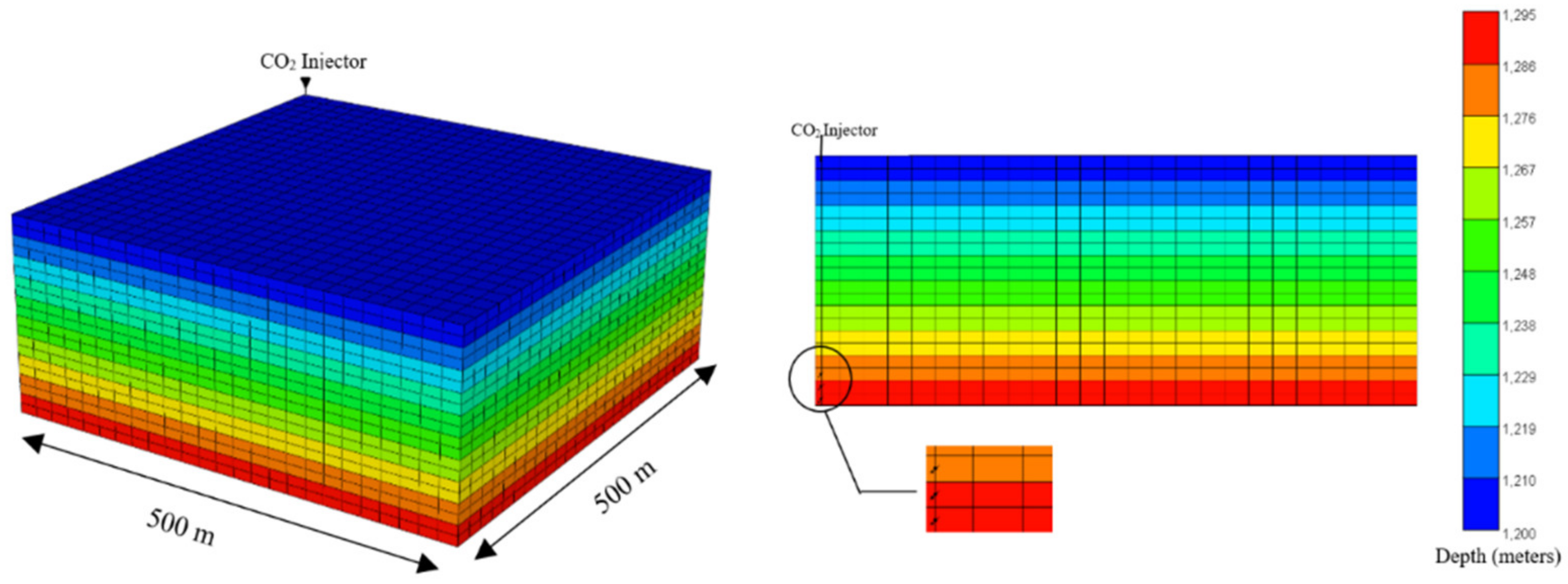
2.1. Reservoir Model

We use a 3D compositional reservoir simulator (CMG-GEM) to model the injection of CO₂ in a synthetic reservoir with a constant boundary. The model describes a multi-component system of brine and CO₂ using component transport equations, thermodynamic equations between the gas and the aqueous phase, and the geochemical reactions that occur during the injection of CO₂ in deep saline aquifers. The governing equation for the process involves basic mass balance equations for each of the major components or the bulk phases in the system [6]. For a closed system with $\alpha$ phases and i components, the accumulation of CO₂ is the summation of convective mass transfer, diffusive/dispersive mass transfer, consumption due to a chemical reaction, and mass of the injected gas. The governing equation is:

$${\displaystyle \sum }_{\alpha }\frac{\partial }{\partial t}{\rho }_{\alpha }\mathsf{\varphi }{s}_{\alpha }{m}_{\alpha }{}^i={\displaystyle \sum }_{\alpha }\nabla \cdot \left({\rho }_{\alpha }{\mathit{u}}_{\alpha }{m}_{\alpha }{}^i+{\mathit{j}}_{\alpha }\right)+r^i+{\psi }_{\alpha }{}^i$$

(1)

with $\rho$ as the phase density, $\mathsf{\varphi }$ as the porosity, s as the phase saturation, m as the phase mass fraction of ith component, u_α as the Darcy or convective flux, j_α as the non-advective flux, rⁱ as the reaction of the ith component, and ${\Psi }_{\alpha }^i$ representing the injected mass.

After injection, the CO₂ dissolves in the aqueous phase and is in thermodynamic equilibrium with the gas phase. The fugacity for the gas phase and the components dissolved in the aqueous phase are calculated using the Peng Robinson Equation of State (PR EOS) and Henry’s law, respectively [41]. The Harvey correlation calculates Henry’s law constant at different temperatures and pressures [41].

Figure 1 illustrates the 3D reservoir model used to model CO₂ injections. The base case model consisted of 12,500 cells divided into a 25 × 25 × 20 grid. The total bulk reservoir volume was 2.5 × 10⁷ m³, while the total pore volume was calculated to be 4.501 × 10⁶ m³. Water–gas contact for the simulated reservoir model was set at 1150 m. The injector was placed at the corner of the model (grid block 1,1,1) with the maximum surface gas rate of 10,000 m³/day and the maximum bottom hole pressure of 44,500 kPa. We used a small reservoir for this study to generate accurate results with a reasonable computational time and it can be easily upscaled for a larger reservoir [42]. The well was perforated from the 18th to the 20th layer with a length of 15m. The allowable injection pressure is generally up to 80% of the rock fracture pressure, as indicated in other works [40,41,42,43,44]. The critical fracture stress in this study was taken according to Lucier et al. [40] for CO₂ injection and storage in the Rose Run Sandstone in eastern Ohio, USA. The input parameters for the saline aquifer model are shown in

Table 1. Saline aquifer system input parameters.

Aquifer Properties	Values
Grid number	12,500 (25 × 25 × 20)
Length (m)	500
Width (m)	500
Depth at the top (m)	1200
Thickness (m)	100
Permeability (md)	100
Porosity	0.18
Salinity (M)	1.7
Component	CO2
Critical Pressure (atm)	72.8
Critical Temperature (K)	304.2
Acentric Factor	0.225
Molecular Weight (g/g-mole)	44.01

.

During the CCS operation in deep saline aquifers, the CO₂ is injected into the pore spaces of rocks previously occupied by saline groundwater. Hence, relative permeability is an important parameter for determining the effective permeability of both CO₂ and brine. Several theoretical and experimental models account for the relative permeability of brine–CO₂ systems. Figure 2 shows the relative permeability curve adapted for the reservoir model [45]. We also used a critical gas saturation of 0.4 during the drainage of the reservoir rock due to the hysteresis.

2.2. Machine Learning Models

The use of machine learning models to solve engineering problems dates to the middle of the 20th century [46]. The following subsections briefly discuss the machine learning models adopted in this study.

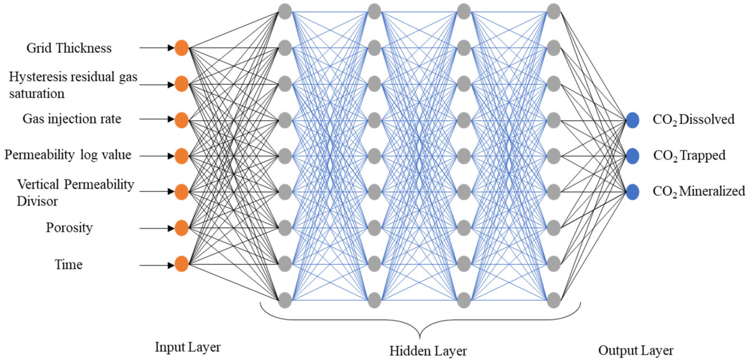
2.2.1. Artificial Neural Networks

The artificial neural network (ANN) or multilayer perceptron (MLP), a sub-field of machine learning and artificial intelligence, deals with algorithms inspired by the biological structure and functioning of human brains to solve complex non-linear problems by using the results from similar past observations [34]. The ANN includes one or more hidden layers, the input layer and the output layer [46]. Recently, ANNs have been applied to solve several complex problems in various petroleum engineering domains such as exploration, reservoir, drilling, and production engineering. In reservoir engineering, ANNs have been successfully applied to reservoir characterization [47,48], estimation of rock and fluid properties [32,48,49,50,51], well testing [52], uncertainty in reservoir performance [53], geomechanical characterization [54], reserves estimation, enhanced oil recovery [55], outlier detection [35], and formation damage estimation [56]. The learning algorithm for ANNs resembles how the brain handles information. A neuron is a basic unit of the brain activated by electrical signals, processes the received signal, and transfers the signals to other neurons. The input signal received by a neuron needs to exceed a certain threshold to be activated and further transmit a signal. In a biological neuron, the nucleus transforms the chemical inputs from the dendrites into signals transferred to the subsequent neurons through the axon terminals [57]. ANNs consist of an interconnected network of neurons with layers of nodes. A complete neural network consists of an input layer aggregating the input signal from other connected neurons, a hidden layer responsible for training, and an output layer. Each node in the hidden layer of an ANN takes the input from the previous layer and passes it to the next layer of nodes by calculating the weights based on the selected activation function. The activation function mimics the complex process of a neural output to the next layer.

The optimum number of hidden layers with neurons is calculated through trial and error, which varies based on the system’s complexity. The proposed MLP model has four hidden layers containing 500 nodes each, as illustrated in Figure 3. We used the tanh activation function in the hidden layer to transform data into higher-order spaces. This study used python’s Scikit-Learn package ‘MLPRegressor’ to develop the MLP model [58]. In addition, the stochastic gradient-based optimizer ‘adam’ was used to obtain the optimal weight values. Mathematically, the output from a node can be represented by:

$$output=\phi \left(W^{T}x+b\right)$$

(2)

where x is the input value from the input layer multiplied by weight w and added with a bias of b and applied to the activation function to $\phi$. The detailed hyperparameters for the MLP model are provided in

Table 2. Parameters used for training the machine learning models.

Models	Prediction Target	Parameters
Random Forest	CO2 Trapped	{‘n_estimators’: 200, ‘min_samples_split’: 2, ‘min_samples_leaf’: 1, ‘max_features’: ‘auto’, ‘max_depth’: None, ‘bootstrap’: True}
	CO2 Mineral
	CO2 Dissolved
XGB	CO2 Trapped	{‘subsample’: 0.7, ‘n_estimators’: 1000, ‘max_depth’: 20, ‘learning_rate’: 0.01, ‘colsample_bytree’: 0.8 ‘colsample_bylevel’: 0.9}
	CO2 Mineral	{‘subsample’: 0.8, ‘n_estimators’: 500, ‘max_depth’: 20, ‘learning_rate’: 0.1, ‘colsample_bytree’: 0.8, ‘colsample_bylevel’: 0.4}
	CO2 Dissolved	{‘subsample’: 0.5, ‘n_estimators’: 1000, ‘max_depth’: 15, ‘learning_rate’: 0.1, ‘colsample_bytree’: 0.9, ‘colsample_bylevel’: 0.9}
SVR	CO2 Trapped	{‘kernel’: ‘rbf’, ‘gamma’: 1, ‘C’: 10}
	CO2 Mineral	{‘kernel’: ‘rbf’, ‘gamma’: 0.1, ‘C’: 100}
	CO2 Dissolved	{‘kernel’: ‘rbf’, ‘gamma’: 0.1, ‘C’: 1000}
MLP	CO2 Trapped	{‘solver’: ‘adam’, ‘max_iter’: 200, ‘learning_rate’: ‘adaptive’, ‘hidden_layer_sizes’: (500, 500, 500, 500), ‘alpha’: 0.0001, ‘activation’: ‘tanh’}
	CO2 Mineral
	CO2 Dissolved

.

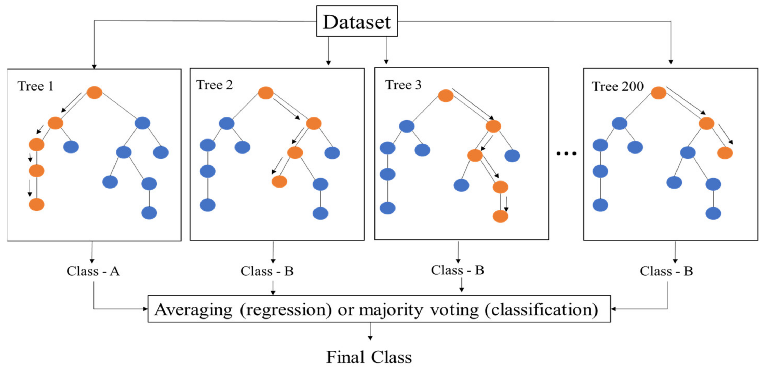
2.2.2. Random Forest

Random forest (RF) is an ensemble-based algorithm based on tree-predictor-based classification [59]. The regression trees are developed using a subset of input variables and training data samples, which offers a stable prediction result and a controlled level of nonlinearity in the training data samples [35,59]. Furthermore, the tree nodes are separated using binary splits, effectively preventing overfitting issues, as illustrated in Figure 4. This study selects 200 decision trees and a minimum number of 2 samples for each leaf node, as shown in Table 2. Each regression decision tree can be trained using sampling bags in the training dataset. In contrast, the prediction errors can be determined using samples without the training dataset, also referred to as out-of-bag (OOB) samples. The mean square error is expressed as follows [38,59]:

$${\mathrm{MSE}}_{\mathrm{Out}\text{-}\mathrm{of}\text{-}\mathrm{bag} \mathrm{Samples}}=\frac{1}{N_T}{{\displaystyle \sum }}_{i=1}^{N_T}(x_i-x_{i_{pred})}{}^2$$

(3)

where N_T is the number of OOB samples, x_i is the sample value, and $x_{i_{pred}}$ is the OOB prediction value. This study used python’s Scikit-Learn package “RandomForestRegressor” to develop the RF model [58].

2.2.3. Support Vector Regression

The basic function of support vector regression (SVR), a popular regression method with a wide range of applications, can be described as following [60]:

g(x) = w^TΦ(x) + a

(4)

where w is the weight factor, x is the input vector, a is the bias, and Φ represents the mapping function. For N_s training samples, the standard formula for SVR is as follows:

$${}_{w, b, \xi ,{\xi }^{*}}{}^{min} \frac{1}{2}{w}^{\mathrm{T}}w+C {\displaystyle \sum }_{i=1}^{N_s}\left({\xi }_i+{\xi }_i^{*}\right)$$

(5)

Subject to:

$$w^{\mathrm{T}}\mathsf{\Phi }\left(x_i\right)+b-y_i{ }_{\le } \epsilon +{\xi }_i,$$

(6)

$$y_i{ }_{-} w^{\mathrm{T}}\mathsf{\Phi }\left(x_i\right) - b{ }_{\le } \epsilon +{\xi }_i^{*},$$

(7)

$${\xi }_i, {\xi }_i^{*} \ge 0, i=1, 2, \dots , N_s$$

(8)

where ${\xi }_i \mathrm{and} {\xi }_i^{*}$ are the slack parameters stating the range of the training errors pointing to an error tolerance of $\epsilon$ [31,60], and C is the penalty parameter. This study used the python’s Scikit-Learn package “SVR” to develop the machine learning model [58]. The default ‘rbf’ kernel was used, whose equation can be described as [31]:

$$\left(x_i,x_j\right)=\exp (-\mathsf{{\rm Y}}\parallel x_i-x_j\parallel {}_2^2, \mathsf{{\rm Y}}>0$$

(9)

The predictive model can be described as below [48]:

$$g\left(x\right)={\displaystyle \sum }_{i=1}^{N_s}\left(-{\alpha }_i+{\alpha }_i^{*}\right)K\left(x_i, x\right)+b$$

(10)

where ${\alpha }_i \mathrm{and} {\alpha }_i^{*}$ are determined by adapting the Lagrange multipliers. Furthermore, the support vectors are the vector for the non-zero component of $\left(-{\alpha }_i+{\alpha }_i^{*}\right)$, i = 1, 2, ..., N_s. The detailed hyperparameters used to train the SVR model are shown in Table 2.

2.2.4. Extreme Gradient Boosting

Extreme gradient boosting, also referred to as XGB, is an ensemble of classification and regression trees methods developed by Chen and Guestrin [61,62]. XGB-based regression creates a step-by-step functionality by adjusting the decision tree proportions based on the previous tree [61,62]. The objective function (K) for round ‘g’ can be expressed by the following formula [61,62]:

$$K^{\left(g\right)}={\displaystyle \sum }_{i=0}^{n}m(y_i+y_p)+{\displaystyle \sum }_{n=1}^p\beta \left(f_p\right)$$

(11)

where f_p is the function for the P-tree, y_i and y_p represent the simulated and predicted values, respectively, and the training loss and regulations are denoted by m and p, respectively. XGB regression optimizes the training loss by adjusting the regression tree models, using the residual and misclassification data from the simulated and predicted datasets [61,62]. The detailed hyperparameters used to train the XGB model are shown in Table 2.

2.3. Hyperparameters

Hyperparameters for a machine learning algorithm are external configurations whose values cannot be estimated from data [63]. The hyperparameters for a model need to be tuned or optimized to improve the learning process. For example, some of the hyperparameters for an artificial neural network (ANN) are the number of layers, nodes, the learning rate, and the activation function (sigmoid, tanh, ReLU, and others). The hyperparameters have a significant effect on the output of an algorithm. The hyperparameters control various metrics or tools (decision boundary) that an algorithm uses to create a proxy model. In advance, we do not know the best values for a model’s hyperparameters [63]. This study used the grid search to identify the optimal set of hyperparameters, resulting in the lowest mean absolute error for a given algorithm. The hyperparameters for each algorithm and their optimal values are summarized in Table 2.

2.4. Evaluation Metrics

Using the iterative models, a large number of datasets were generated to develop, train, and validate the machine learning models. Then, the data were preprocessed with feature scaling before training the predictive models. Feature scaling transforms the input and the output data into the same scale, significantly improving the performance and training stability of the model. In this study, the data normalization was done into a standard range of −1 and 1 by using the following formula:

$$x^{\prime }=2\left(\frac{x-\min (x)}{\max (x)-\min (x)}\right)-1$$

(12)

where x is the original value of the given parameter, $x’$ is the scaled value of x, min(x) in the minimum value of x, and max(x) is the maximum value of x. The training set included 75% of the randomly selected data in this study, while the test phase included the remaining 25% of the data. We used the K-fold (k = 5) cross-validation method for hyperparameter tuning and testing the accuracy of the trained models (more on this in Section 3.2). The performance of the developed machine learning models was evaluated using various statistical indexes described below:

1.

Coefficient of Determination (R²)

$${\mathrm{R}}^2=1-\frac{{{\displaystyle \sum }}_{i=1}^n(y_{i_{sim}}-y_{i_{pred})}{}^2}{{{\displaystyle \sum }}_{i=1}^n{(y_{i_{pred}}-\overline{y})}^2}$$

(13)

2.

Root Mean Square Error (RMSE)

$$\mathrm{RMSE}=\sqrt{\frac{1}{n}{{\displaystyle \sum }}_{i=1}^n(y_{i_{sim}}-y_{i_{pred})}{}^2}$$

(14)

3.

Average Absolute Relative Error (AARE)

$$\mathrm{AARE} (\%)=\frac{1}{n}{{\displaystyle \sum }}_{i=1}^n\left|\frac{(y_{i_{sim}}-y_{i_{pred})}}{y_{i_{sim}}}\right|\times 100$$

(15)

where $\overline{y}$ indicates the average value and $y_{i_{sim}}$ and $y_{i_{pred}}$ denote the simulated and predicted values, respectively.

3. Results

The reservoir was injected with CO₂ for 25 years, after which it was monitored for the next 275 years. Figure 5 shows the 3D CO₂ saturation profile for the reservoir after five years, twenty years, fifty years, one hundred years, two hundred years, and three hundred years, respectively. To generate the 3D view, we considered only the grid blocks where the impact of gas saturation was noticeable. This study considered three major CO₂ trapping mechanisms: residual trapping, dissolution trapping, and mineral trapping. At the beginning of the injection period, most of the CO₂ is trapped due to capillary trapping or residual trapping. However, as the density of the supercritical CO₂ is considerably lower than the brine density (950–1250 kg/m³), most of the CO₂ rises upward within the aquifer until it reaches an impermeable horizontal caprock and is structurally trapped. The supercritical CO₂ may further spread laterally over a large area due to its buoyancy, the lateral movement of the aquifer, and the slope of the caprock until it experiences another vertical trap [64]. After a significant amount of time, the structurally trapped CO_2, which is in contact with the brine, slowly dissolves by molecular diffusion, resulting in the dissolution trapping. Thus, there is a noticeable decrease in the rate of CO₂ residual trapping throughout time, whereas the solubility of CO₂ trapping increases gradually. Dissolution trapping is one of the most dominant storage mechanisms with the maximum storage security of CO₂ in a reservoir [5]. The brine–CO₂ solution is slightly denser than the pure brine by a factor of 0.1–0.2%, depending on conditions in the aquifer [64,65]. This density gradient between the top layer and the layer immediately below it creates a buoyant instability which results in convective mixing. The CO₂-rich layer at the top sinks to the bottom of the aquifer and is replaced by fresh brine. This process creates a loop migrating the free CO₂ trapped as a separate phase to the bottom of the aquifer as the brine–CO₂ solution. Although difficult to quantify, convective mixing is hypothesized to increase CO₂ storage in saline aquifers [64,65] significantly. However, vertical and horizontal permeability anisotropy (heterogeneities) present in the porous media further complicates the spatial and temporal aspects of CO₂ dissolution in brine [65]. Finally, the geochemical properties of the brine and the reservoir may also significantly enhance the transfer of supercritical CO₂ due to mineral trapping [66]. The dissolution of CO₂ into the brine is vital to prevent the possibility of CO₂ leakage from the faults and cracks that may be present in the geological seal.

Figure 6 describes the change in the CO₂ trapping mechanisms throughout time. The trapping mechanisms are expressed in terms of the Residual Gas Trapping Index (RTI), Solubility Gas Trapping Index (STI), and Mineralized Trapping Index (MTI), indicated in fraction. The RTI, STI, and MTI are defined by the following equations [67]:

$$\mathrm{RTI}=\frac{\mathrm{The} \mathrm{total} \mathrm{mass} \mathrm{of} \mathrm{trapped} \mathrm{residual} {\mathrm{CO}}_2}{\mathrm{The} \mathrm{total} \mathrm{mass} \mathrm{of} \mathrm{injected} {\mathrm{CO}}_2}$$

(16)

$$\mathrm{STI}=\frac{\mathrm{The} \mathrm{total} \mathrm{mass} \mathrm{of} {\mathrm{CO}}_2 \mathrm{dissolved} \mathrm{in} \mathrm{brine}}{\mathrm{The} \mathrm{total} \mathrm{mass} \mathrm{of} \mathrm{injected} {\mathrm{CO}}_2}$$

(17)

$$\mathrm{MTI}=\frac{\mathrm{The} \mathrm{total} \mathrm{mass} \mathrm{of} {\mathrm{CO}}_2 \mathrm{mineralized}}{\mathrm{The} \mathrm{total} \mathrm{mass} \mathrm{of} \mathrm{injected} {\mathrm{CO}}_2}$$

(18)

Figure 6 shows that, throughout time, the effect of the RTI decreased, whereas the impact of the STI increased gradually. The effect of the MTI was negligible in the initial portion of the simulation. However, since mineral trapping is the most secure method of safe storage of CO₂, this study includes the effect of the MTI. It should be noted that the impact of the MTI will increase throughout time and will be more significant after a long period [66].

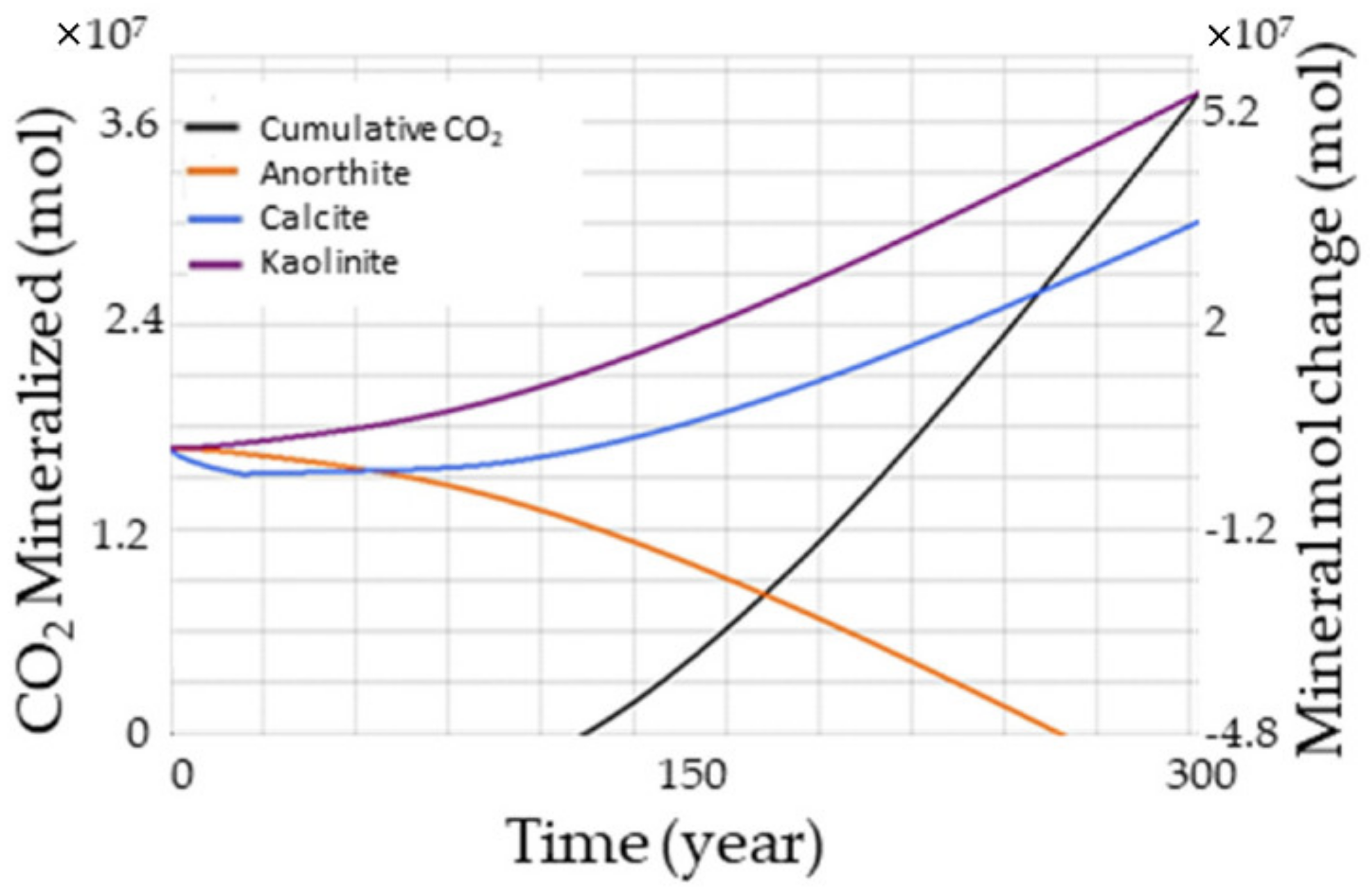
3.1. Effect of Mineralization in CO₂ Trapping

Mineral trapping offers the advantage of an increased storage capacity and CO₂ immobilization for a long period [66]. Even though mineralization takes a long time, the trapping process can be sped up by finding optimal parameters, including the system pressure and temperature, brine composition, pH, sweep efficiency, reservoir formation, mineral trapping kinetics, and stress impact on the caprock [68,69,70,71,72]. Figure 7 illustrates the amount of carbon dioxide mineralized throughout time. We considered only three minerals for this study to reduce the computational time: anorthite, calcite, and kaolinite. The chemical reactions for these minerals are as follows:

Anorthite + 8H⁺ = 4H₂O + Ca⁺⁺ + 2Al⁺⁺⁺ + 2SiO₂ (aq)
Calcite + H⁺ = Ca⁺⁺ + HCO₃⁻
Kaolinite + 6H⁺ = 5H₂O + 2Al⁺⁺⁺ + 2SiO₂ (aq)

From Figure 7, while anorthite was getting dissolved, kaolinite got precipitated throughout the time. Meanwhile, calcite got dissolved at the initial portion of the simulation but started to precipitate later. This indicates that the impact of the MTI, shown in Figure 6, was slightly higher than observed since only the precipitated amount could be calculated for measuring the MTI. Therefore, the full effect of the mineralization could only be discovered by looking at the mineralization of the individual mineral forms. Figure 7 also shows that the non-zero CO₂ trapping from mineralization was only observed after almost 100 years.

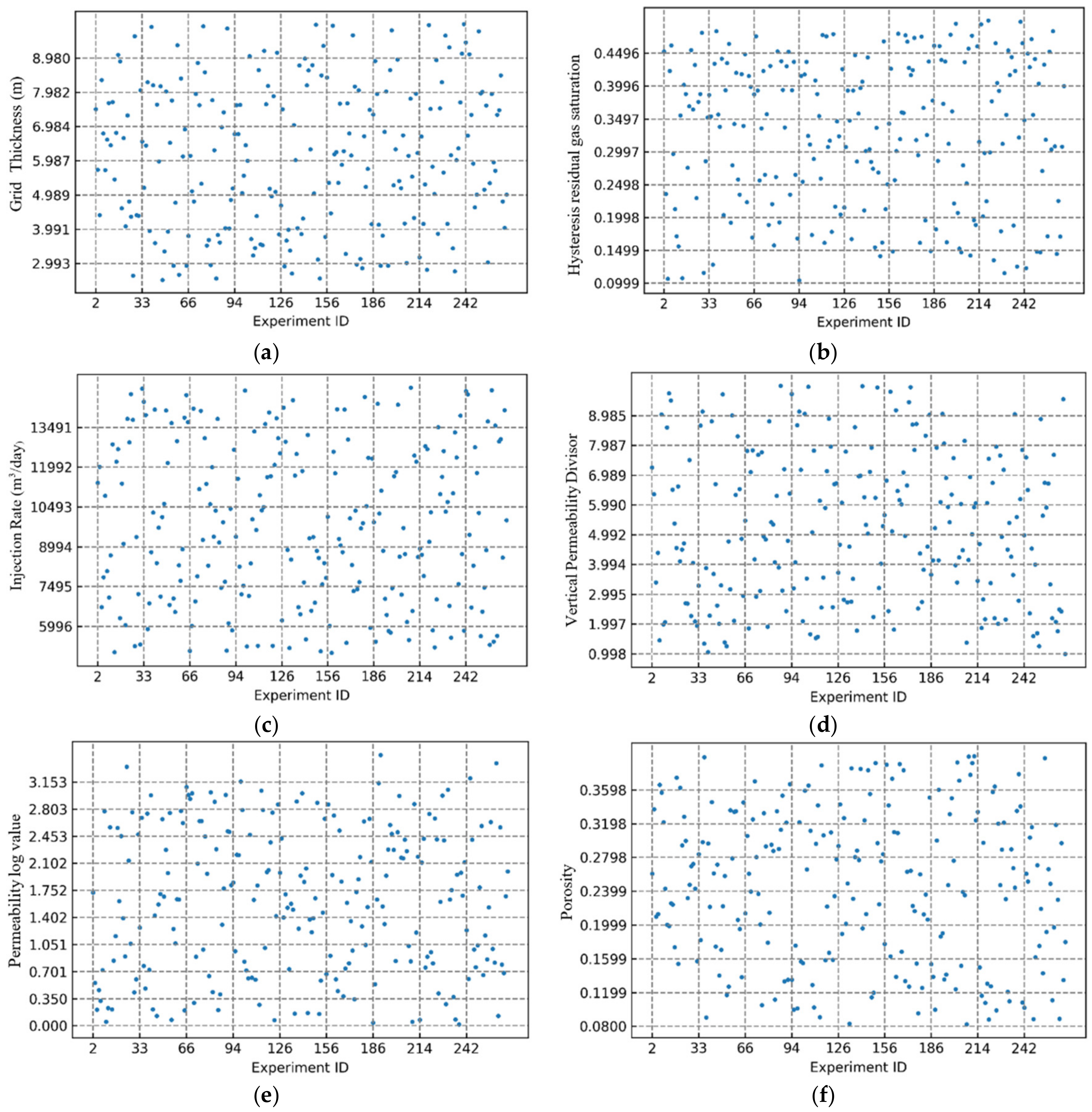
3.2. Data for Proxy Model

We generated numerous iterations of the base case model of the reservoir by modifying various uncertain properties and decision parameters. Seven input parameters were considered for the iterations. The CO₂ sequestered after each five-year interval was used as one of the parameters for the total dissolved CO₂. The addition of the time parameter allowed for the calculation of the intermediate CO₂ sequestered at different time intervals instead of just the final simulation period. In total, 19,800 data points were used for training and testing the model. In order to avoid bias during the selection of the training and testing data, we used a five-fold cross-validation method. For the five-fold cross-validation method, the initial dataset was randomly split into five folds. Each of the five sets was then used as the test set, and the other four sets were used as training data to fit the model. The test set was then used to evaluate the quality of the generated proxy model. In the subsequent iteration, a new test set was selected from one of the five folds. This continued for all the folds so that all the samples in the dataset were predicted by using a model generated without themselves in the training data. The cross-validation method used here reduced the risk of both bias and overfitting, and the entire dataset could be utilized as a test dataset. The statistical overview of the input parameters distribution is provided in

Table 3. Statistical overview of the input parameters distribution.

Input Parameters	Base Case Model Value	Minimum Value	Maximum Value
Grid Thickness (m)	5	2.5	10
Hysteresis residual gas saturation	0.4	0.1	0.5
Gas Injection Rate (m3/day)	10,000	5000	15,000
Permeability log value	2	0	3.69897
Vertical Permeability Divisor a		1	10
Porosity	0.18	0.08	0.4
Time (year) b	300	5	300

^a Higher vertical permeability divisor indicates a lower permeability; ^b total trapping is considered at each of the 5-year intervals.

. Furthermore, the input parameters distribution generated by the randomized process can be observed in Figure 8, where experiment ID denotes the iterative model number.

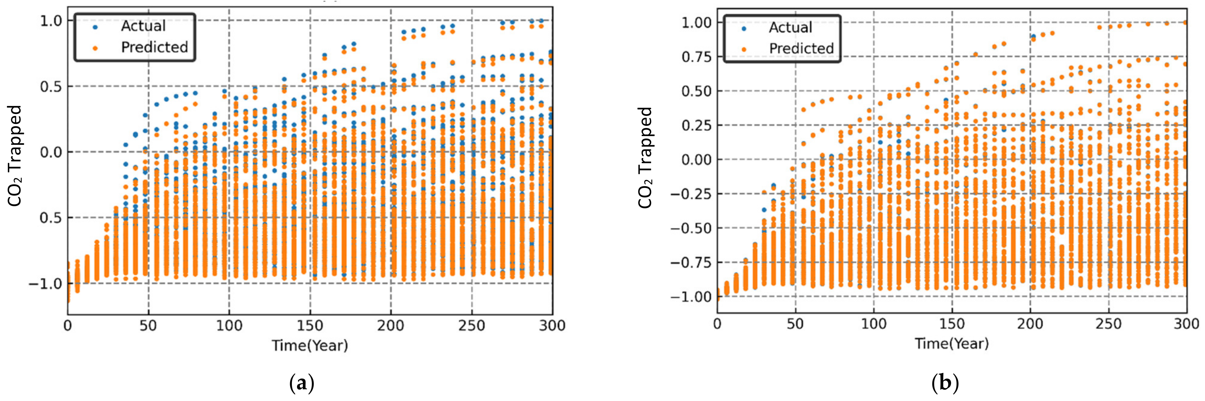
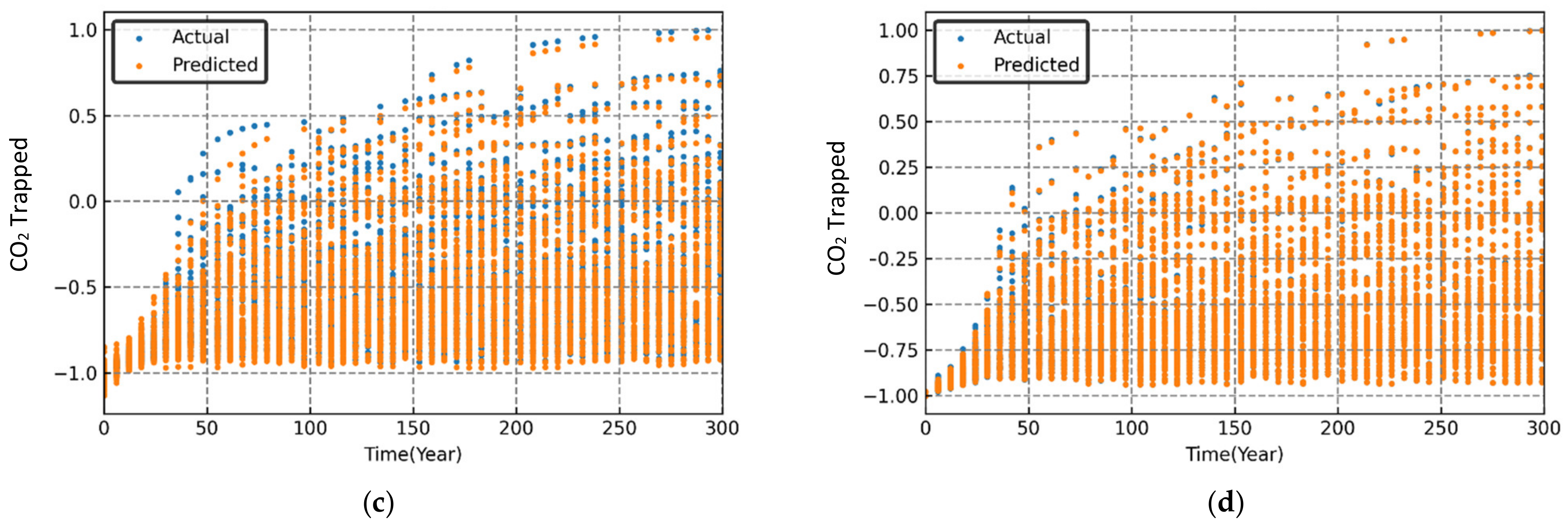
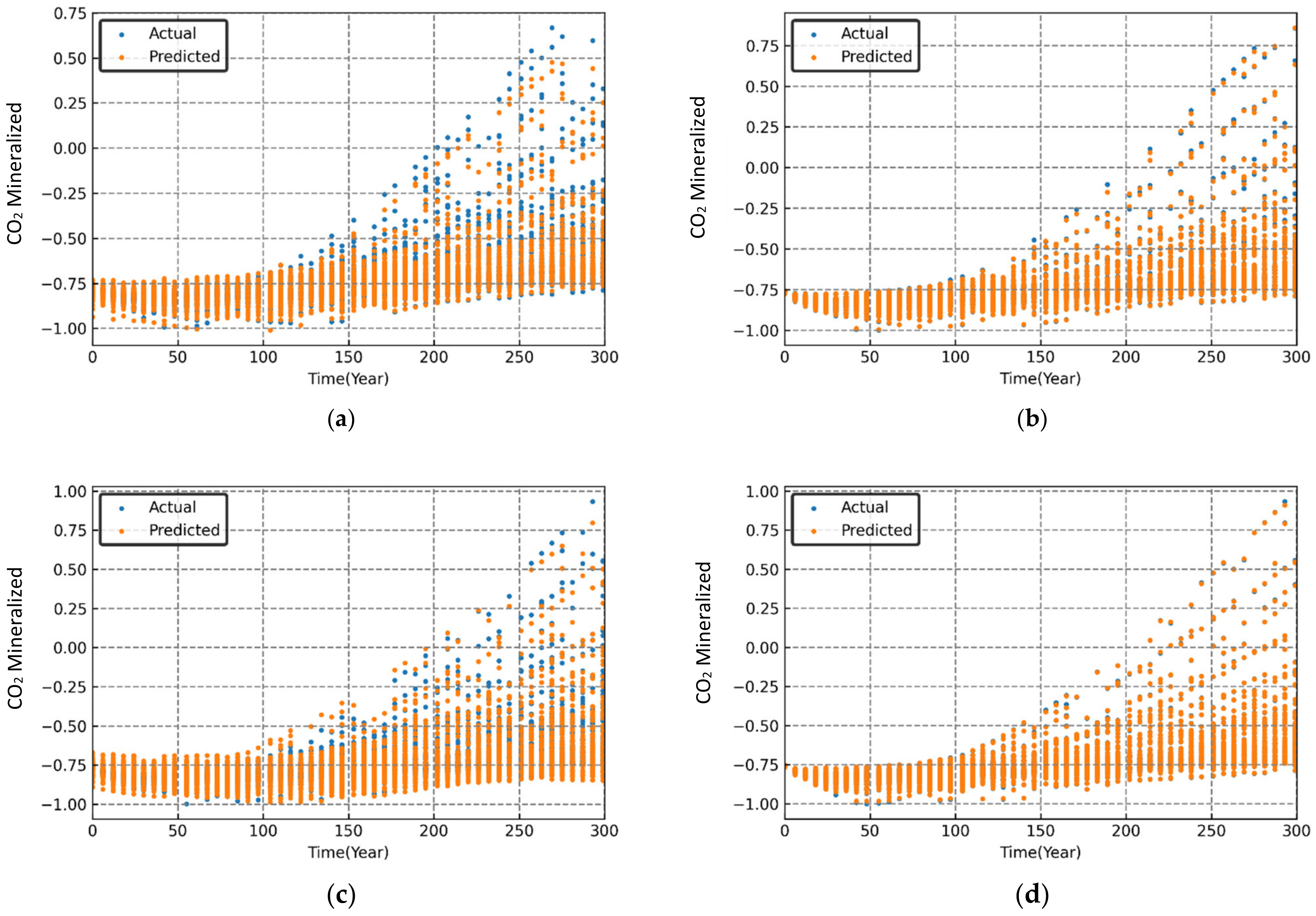
3.3. Results for Proxy Models

The performance evaluation of each machine learning model was conducted through graphical and statistical error analysis. Figure 9, Figure 10 and Figure 11 present the cross-validated results for dissolved, mineralized, and trapped CO₂ (normalized) for different sets of the randomized input parameters. The model was deemed to be highly accurate if the actual and the predicted data points coincided on top of each other. As seen in Figure 9, Figure 10 and Figure 11, both the RF and XGB models had a slightly better performance in predicting the CO₂ sequestered compared to the MLP and SVR models.

This was further indicated by the compact distribution of the data points for the RF and XGB models in the predicted vs observed plots shown in Figure 12, Figure 13 and Figure 14.

For a better assessment of the CO₂ trapping prediction performance of the four machine learning methods, the statistical accuracy of each method is provided in

Table 4. The statistical accuracy of the proposed machine learning methods in determining CO₂ Trapped, CO₂ Dissolved, and CO₂ Mineralized.

Models	Target	Training Results			Validation with Test Dataset
		R2	RMSE	AARE	R2	RMSE	AARE
LR	CO2 Trapped	0.50124	1.38554	1.91973	0.50781	1.26611	1.60303
	CO2 Mineral	0.50491	0.50656	0.25660	0.47804	0.49898	0.24898
	CO2 Dissolved	0.71762	0.70373	0.49523	0.71366	0.63791	0.40693
RF	CO2 Trapped	0.99995	0.07979	0.00637	0.99972	0.14946	0.02234
	CO2 Mineral	0.99991	0.05562	0.00309	0.99946	0.09164	0.00840
	CO2 Dissolved	0.99996	0.06801	0.00462	0.99969	0.12805	0.01640
XGB	CO2 Trapped	0.99999	0.05452	0.00297	0.99988	0.08690	0.00755
	CO2 Mineral	0.99997	0.03957	0.00157	0.99968	0.07606	0.00579
	CO2 Dissolved	0.99999	0.04130	0.00171	0.99985	0.07781	0.00605
SVR	CO2 Trapped	0.96633	0.67665	0.45786	0.96732	0.72408	0.52429
	CO2 Mineral	0.88767	0.29034	0.08430	0.89275	0.27896	0.07782
	CO2 Dissolved	0.95176	0.41113	0.16903	0.94668	0.41114	0.16904
MLP	CO2 Trapped	0.99185	0.38120	0.14531	0.99164	0.40102	0.16082
	CO2 Mineral	0.98450	0.16825	0.02831	0.98391	0.18950	0.03591
	CO2 Dissolved	0.96463	0.33920	0.11506	0.96700	0.35014	0.12260

in terms of the R²_, RMSE, and AARE values. In addition, the accuracy of the simple linear regression (model) is also provided for comparative purposes. The XGB model had the best CO₂ trapping performance prediction with R² values of 0.99996, 0.99990, and 0.99996 for CO₂ trapped, CO₂ mineralized, and CO₂ dissolved, respectively. Furthermore, the RF model also had excellent CO₂ trapping performance with R² values of 0.99989, 0.99980, and 0.99989 for CO₂ trapped, CO₂ mineralized, and CO₂ dissolved, respectively. Finally, the MLP model had an acceptable prediction performance with an R² value of over 0.9 for all trapping scenarios. The results presented here show that RF and XGB had better predictive ability than MLP, compared to the prior studies [38,39,67]. Additionally, both RF and XGB yielded reliable results and should be chosen based on the quality/volume of the training data. As RF is more computationally efficient than XGB [73], a negligible loss in accuracy to improve the training and testing time may be acceptable by using RF over XGB.

The cumulative frequency of the Absolute Relative Error (ARE) distributions of the CO₂ dissolved, CO₂ trapped, and CO₂ mineralized values are shown in Figure 15a–c, respectively. We also compared the results from more sophisticated models to linear regression (LR) in Figure 15. The results showed that more than 90% of the cases could be predicted with an ARE of less than 10%. Furthermore, considering the graphical error analysis and statistical index indicators, the machine learning models were ranked as XGB > RF > MLP > SVR, based purely on accuracy (disregarding the computational time).

Next, we calculated the feature importance plot for the two best performing machine learning models evaluated in this study (RF and XGB). Figure 16 shows the feature importance plot for CO₂ dissolved, CO₂ trapped, and CO₂ mineralized, respectively. The features are arranged in descending order based on their importance for RF algorithm. For RF, time was the variable that had the most significant impact on all the trapping mechanisms followed by relative permeability hysteresis, permeability, reservoir (grid) thickness, porosity, injection rate, and vertical permeability anisotropy (PermK Div.). For XGB, however, the order of feature importance was not as straightforward, with different variables being significant depending on the trapping mechanism. Figure 16 also provides an insight that the injection rate was not a significant feature in predicting the CO₂ sequestered for both algorithms.

3.4. Application of the Workflow for a Field Case

Although this study only presents results from simulated data, the workflow presented here can be adapted to generate valuable insights for a real aquifer. For the reservoirs with preliminary data, this workflow can help in performing uncertainty analysis and optimization studies. Such results are essential to stay on track with project economics and timelines. Although this study presents results for five machine learning methods (including the linear regression), this workflow is also applicable when applied to other statistical tools such as the design of experiments (DOE) and response surface modeling (RSM). The proxy models should be carefully validated in order to avoid overfitting and underfitting. However, some algorithms may result in proxy models that cannot capture the complexity of the physics behind the aquifer model (Table 4, LR and SVR). For the reservoirs where no field data exists, it is recommended that the initial analysis is performed by using data from analogous formations to generate the training data. The initial model can be updated to reflect the new information as more data becomes available.

4. Conclusions

This study assessed the performance of different ML methods in accurately predicting the CO₂ trapping scenarios in a proxy model for a deep saline aquifer. Moreover, CO₂ mineralization effects and CO₂ dissolution and trapping mechanisms are discussed. Based on the findings of this work, the following key conclusions can be drawn:

• A proxy saline aquifer model, developed using a large set of simulated data, can be used to forecast the CO₂ sequestered using various trapping mechanisms with good accuracy. Compared to the reservoir simulation method, these robust models will save time and resources. However, it should be noted that the predictive model is valid for similar geological formations and within the range of input parameters adopted in the current study. The modeling procedures can be easily adapted or reproduced for other real-world scenarios.
• Solubility or dissolution trapping is the most dominant mechanism for CO₂ sequestration (Figure 6).
• CO₂ mineralization is very slow and positive CO2 sequestration is only seen after 100 years of simulation period (Figure 7).
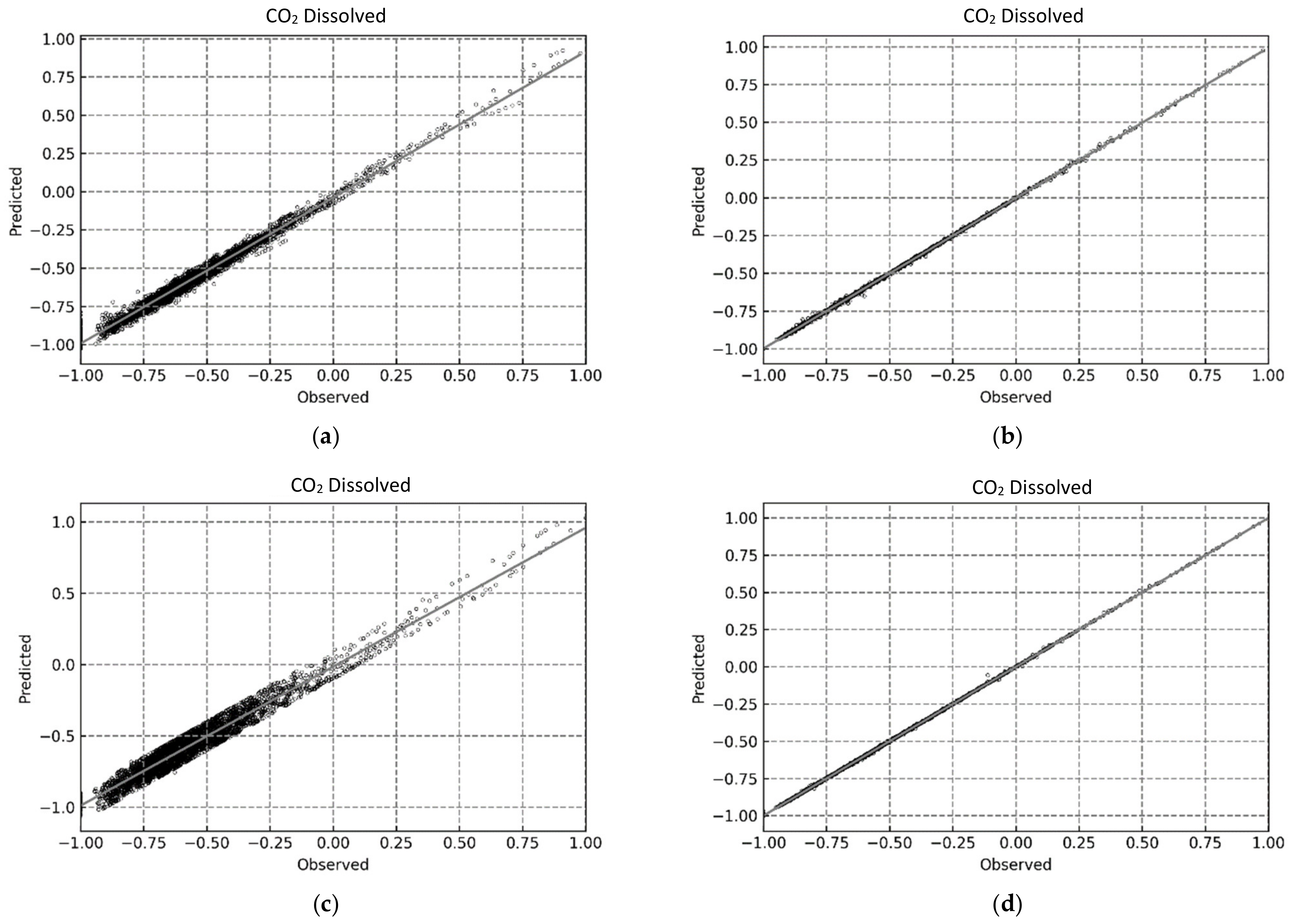
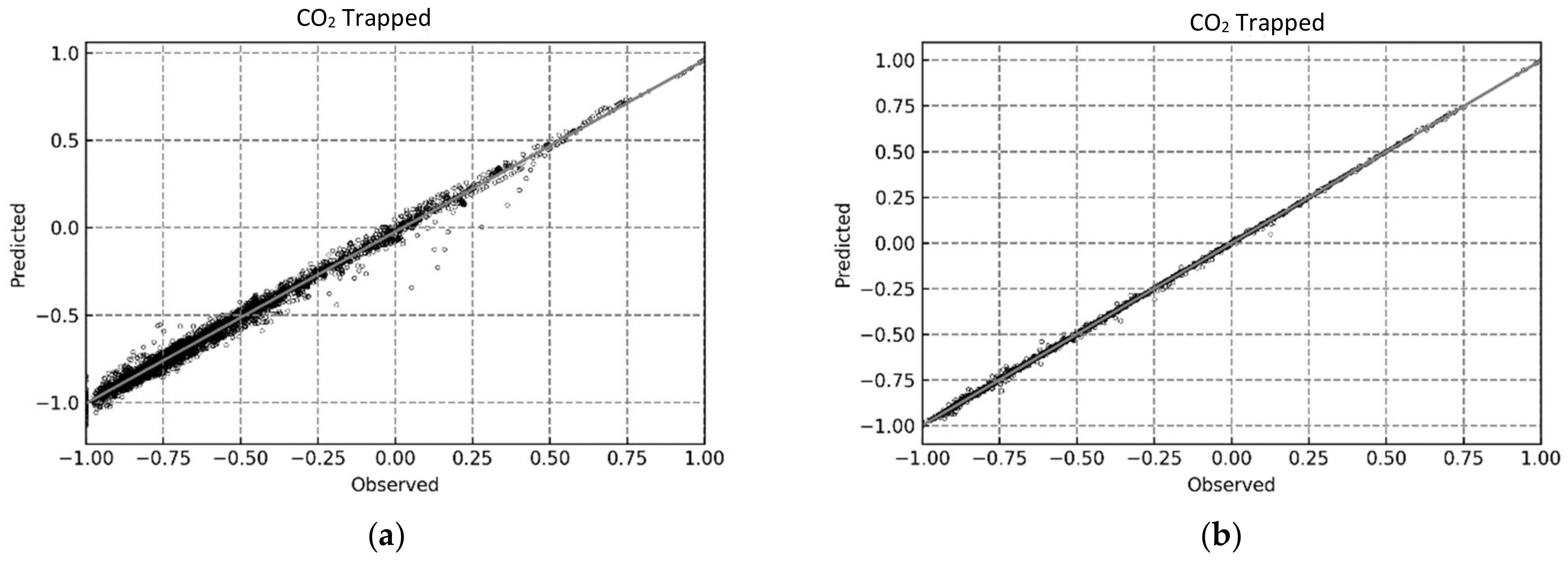
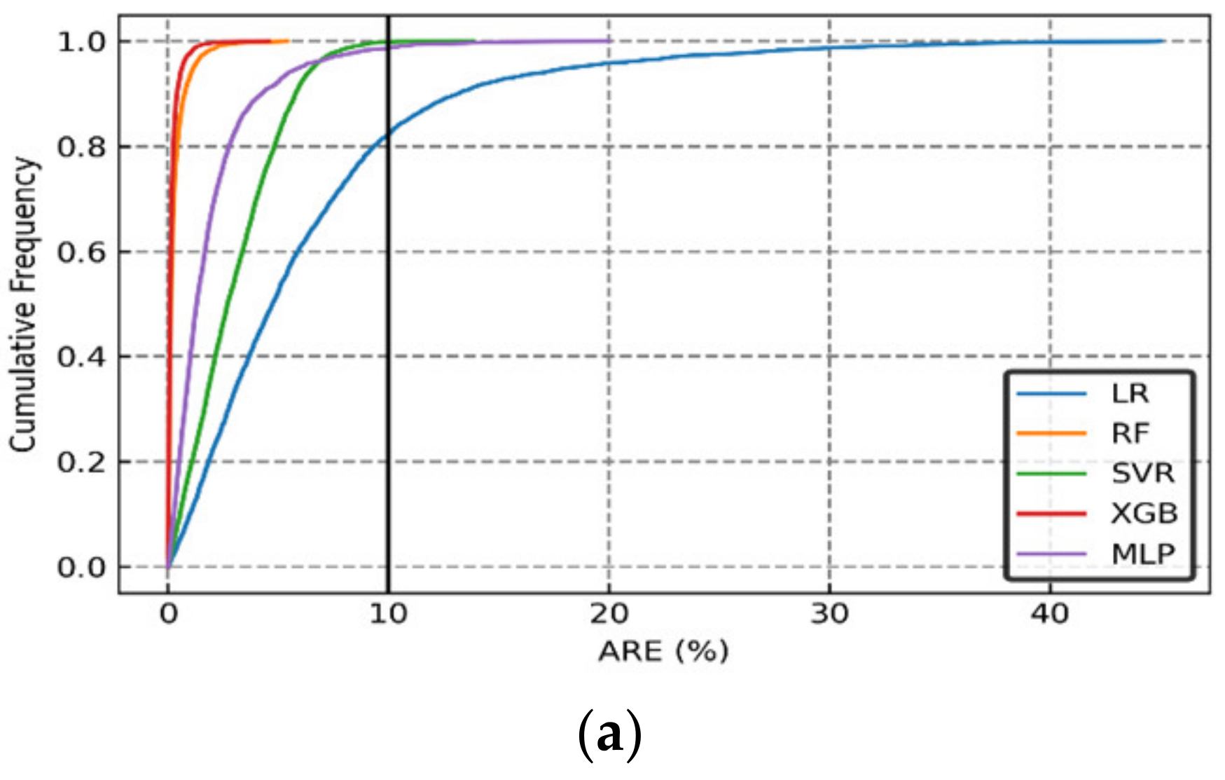
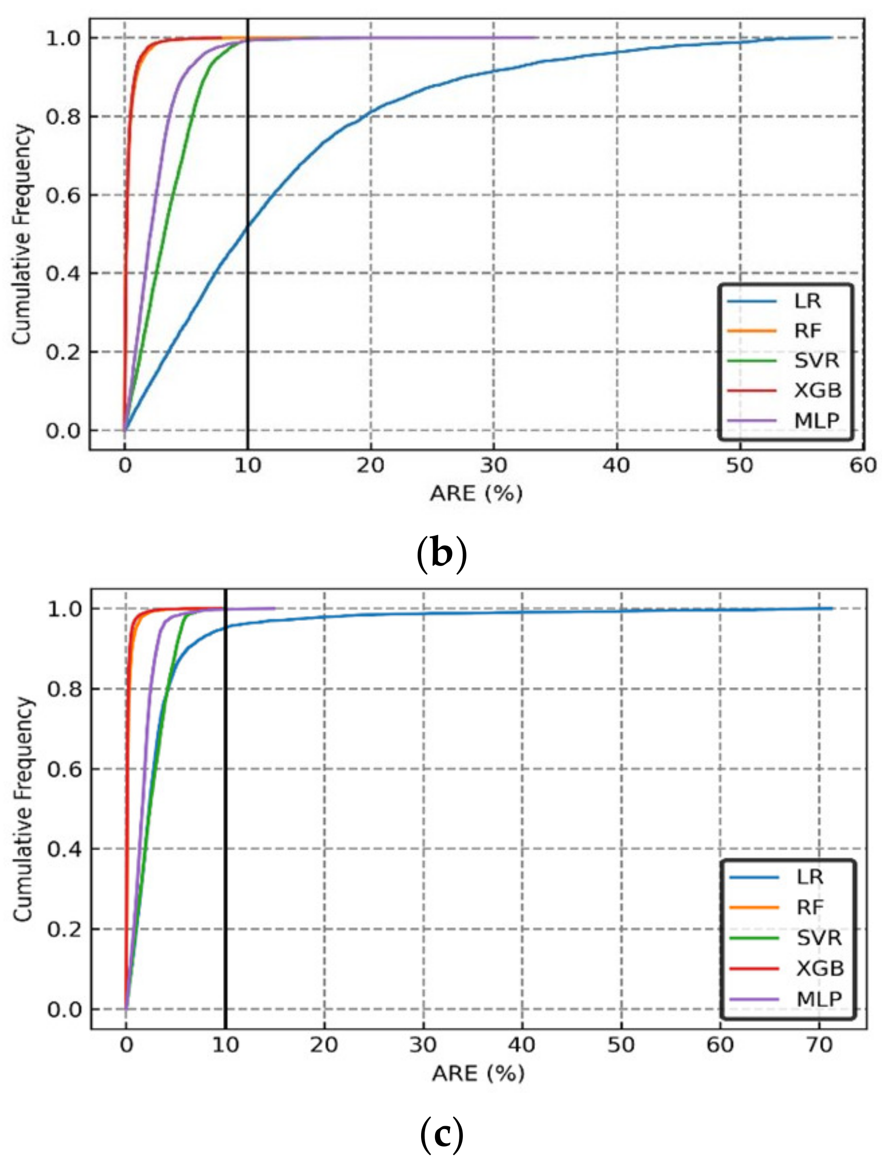
• Four different ML methods (RF, XGB, SVR, and MLP) were evaluated to predict the CO₂ dissolved, mineralized, and trapping scenarios. In addition, the accuracy of simple linear regression (model) was also provided for comparative purposes. Based on the statistical accuracy results during the validation of the ML models, both RF and XGB had better predictive ability than the MLP models (Table 4). The proposed XGB model had the best CO₂ trapping performance prediction with R² values of 0.99988, 0.99968, and 0.99985 for the CO₂ trapped, CO₂ mineralized, and CO₂ dissolved scenarios, respectively. Meanwhile, RF also showed promising results, with R² values of 0.99972, 0.99946, and 0.99969 for the same trapping mechanisms, respectively.
• Both the proposed RF and XGB models can be considered robust CO₂ trapping prediction tools for saline aquifers with similar geological characteristics. Nevertheless, a suitable method should be selected based on the quality/volume of the training data.
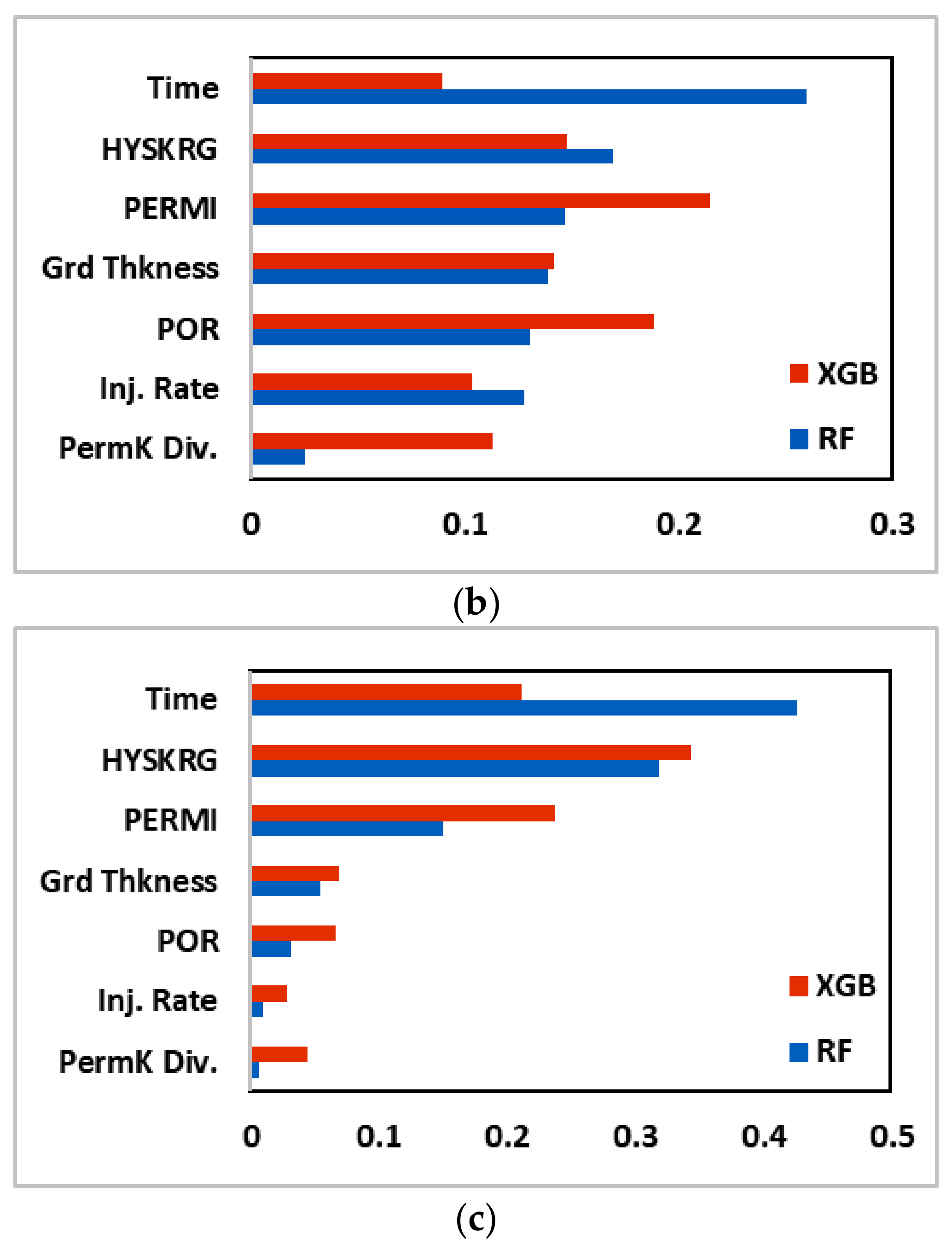
• The rate of CO₂ injection did not show a significant impact on any of the CO₂ trapping mechanisms (Figure 16). However, further studies are required to fully evaluate and conclude the effect of the injection rate on CO₂ sequestration using various trapping mechanisms.

References

1. Mkemai, R.M.; Bin, G. A modeling and numerical simulation study of enhanced CO2 sequestration into deep saline formation: A strategy towards climate change mitigation. Mitig. Adapt. Strat. Glob. Chang. 2020, 25, 901–927. [Google Scholar] [CrossRef]
2. Betts, R. Met Office: Atmospheric CO2 Now Hitting 50% Higher Than Pre-Industrial Levels. Available online: https://www.carbonbrief.org/met-office-atmospheric-co2-now-hitting-50-higher-than-pre-industrial-levels/ (accessed on 9 June 2022).
3. U.S. Energy Information Administration. Annual Energy Outlook 2020 with Projections to 2050; (No. AEO2020); U.S. Energy Information Administration: Washington, DC, USA, 2020.
4. Szulczewski, M.L.; MacMinn, C.W.; Herzog, H.J.; Juanes, R. Lifetime of carbon capture and storage as a climate-change mitigation technology. Proc. Natl. Acad. Sci. USA 2012, 109, 5185–5189. [Google Scholar] [CrossRef] [PubMed] [Green Version]
5. Ranganathan, P.; Farajzadeh, R.; Bruining, H.; Zitha, P.L.J. Numerical Simulation of Natural Convection in Heterogeneous Porous media for CO2 Geological Storage. Transp. Porous Media 2012, 95, 25–54. [Google Scholar] [CrossRef] [Green Version]
6. Celia, M.A.; Bachu, S.; Nordbotten, J.M.; Bandilla, K.W. Status of CO2storage in deep saline aquifers with emphasis on modeling approaches and practical simulations. Water Resour. Res. 2015, 51, 6846–6892. [Google Scholar] [CrossRef]
7. Folger, P. Carbon Capture and Sequestration (CCS) in the United States; Congressional Research Service: Washington, DC, USA, 2018.
8. Seo, J.G.; Mamora, D.D. Experimental and Simulation Studies of Sequestration of Supercritical Carbon Dioxide in Depleted Gas Reservoirs. J. Energy Resour. Technol. Trans. ASME 2005, 127, 1–5. [Google Scholar] [CrossRef] [Green Version]
9. Merey, Ş.; Sinayuc, C. Analysis of carbon dioxide sequestration in shale gas reservoirs by using experimental adsorption data and adsorption models. J. Nat. Gas Sci. Eng. 2016, 36, 1087–1105. [Google Scholar] [CrossRef]
10. Steel, L.; Liu, Q.; Mackay, E.; Maroto-Valer, M.M. CO2 solubility measurements in brine under reservoir conditions: A comparison of experimental and geochemical modeling methods. Greenh. Gases: Sci. Technol. 2016, 6, 197–217. [Google Scholar] [CrossRef]
11. Metz, B.; Davidson, O.; De Coninck, H.C.; Loos, M.; Meyer, L. IPCC Special Report on Carbon Dioxide Capture and Storage; Prepared by Working Group III of the Intergovernmental Panel on Climate Change; Metz, B., Ed.; Cambridge University Press: Cambridge, UK, 2005. [Google Scholar]
12. Alcalde, J.; Flude, S.; Wilkinson, M.; Johnson, G.; Edlmann, K.; Bond, C.E.; Scott, V.; Gilfillan, S.M.V.; Ogaya, X.; Haszeldine, R.S. Estimating geological CO2 storage security to deliver on climate mitigation. Nat. Commun. 2018, 9, 2201. [Google Scholar] [CrossRef]
13. Doranehgard, M.H.; Dehghanpour, H. Quantification of convective and diffusive transport during CO2 dissolution in oil: A numerical and analytical study. Phys. Fluids 2020, 32, 085110. [Google Scholar] [CrossRef]
14. Foroozesh, J.; Moghaddam, R.N. The Convective-Diffusive Mechanism in CO2 Sequestration in Saline Aquifers: Experimental and Numerical Simulation Study. In EUROPEC 2015; European Commission: Brussels, Belgium, 2015; Volume 2015, pp. 165–177. [Google Scholar] [CrossRef]
15. Kneafsey, T.J.; Pruess, K. Laboratory experiments and numerical simulation studies of convectively enhanced carbon dioxide dissolution. Energy Procedia 2011, 4, 5114–5121. [Google Scholar] [CrossRef] [Green Version]
16. Pruess, K. Numerical studies of fluid leakage from a geologic disposal reservoir for CO2 show self-limiting feedback between fluid flow and heat transfer. Geophys. Res. Lett. 2005, 32, 1–4. [Google Scholar] [CrossRef] [Green Version]
17. Kong, X.-Z.; Saar, M.O. Numerical study of the effects of permeability heterogeneity on density-driven convective mixing during CO2 dissolution storage. Int. J. Greenh. Gas Control 2013, 19, 160–173. [Google Scholar] [CrossRef]
18. Kumar, A.; Noh, M.; Pope, G.; Sepehrnoori, K.; Bryant, S.; Lake, L. Reservoir Simulation of CO2 Storage in Deep Saline Aquifers. In Proceedings of the DOE 14th Symposium on Improved Oil Recovery, Tulsa, OK, USA, 17–21 April 2004. [Google Scholar] [CrossRef]
19. Xu, T.; A Apps, J.; Pruess, K. Numerical simulation of CO2 disposal by mineral trapping in deep aquifers. Appl. Geochem. 2004, 19, 917–936. [Google Scholar] [CrossRef]
20. Birkholzer, J.T.; Zhang, Y. The Impact of Fracture–Matrix Interaction on Thermal–Hydrological Conditions in Heated Fractured Rock. Vadose Zone J. 2006, 5, 657–672. [Google Scholar] [CrossRef]
21. Bryant, S.L.; Lakshminarasimhan, S.; Pope, G.A. Buoyancy-Dominated Multiphase Flow and Its Effect on Geological Sequestration of CO2. SPE J. 2008, 13, 447–454. [Google Scholar] [CrossRef]
22. Doughty, C. Investigation of CO2 Plume Behavior for a Large-Scale Pilot Test of Geologic Carbon Storage in a Saline Formation. Transp. Porous Media 2010, 82, 49–76. [Google Scholar] [CrossRef] [Green Version]
23. Hesse, M.A.; Orr, F.M., Jr.; Tchelepi, H.A. Gravity currents with residual trapping. Energy Procedia 2009, 1, 3275–3281. [Google Scholar] [CrossRef] [Green Version]
24. Jiang, X. A review of physical modelling and numerical simulation of long-term geological storage of CO2. Appl. Energy 2011, 88, 3557–3566. [Google Scholar] [CrossRef]
25. Ahmmed, B.; Appold, M.S.; Fan, T.; McPherson, B.J.; Grigg, R.B.; White, M.D. Chemical effects of carbon dioxide sequestration in the Upper Morrow Sandstone in the Farnsworth, Texas, hydrocarbon unit. Environ. Geosci. 2016, 23, 81–93. [Google Scholar] [CrossRef]
26. Pan, F.; McPherson, B.J.; Esser, R.; Xiao, T.; Appold, M.S.; Jia, W.; Moodie, N. Forecasting evolution of formation water chemistry and long-term mineral alteration for GCS in a typical clastic reservoir of the Southwestern United States. Int. J. Greenh. Gas Control 2016, 54, 524–537. [Google Scholar] [CrossRef] [Green Version]
27. Khan, R. Evaluation of the Geologic CO2 Sequestration Potential of the Morrow B Sandstone in the Farnsworth. Ph.D. Thesis, University of Missouri-Columbia, Columbia, MO, USA, 2017. [Google Scholar]
28. Bao, K.; Yan, M.; Allen, R.; Salama, A.; Lu, L.; Jordan, K.E.; Sun, S.; Keyes, D.E. High-Performance Modeling of Carbon Dioxide Sequestration by Coupling Reservoir Simulation and Molecular Dynamics. SPE J. 2016, 21, 0853–0863. [Google Scholar] [CrossRef] [Green Version]
29. Zhang, D.; Song, J. Mechanisms for Geological Carbon Sequestration. Procedia IUTAM 2014, 10, 319–327. [Google Scholar] [CrossRef] [Green Version]
30. Al-Khdheeawi, E.; Vialle, S.; Barifcani, A.; Sarmadivaleh, M.; Iglauer, S. Impact of Injection Scenario on CO2 Leakage and CO2 Trapping Capacity in Homogeneous Reservoirs. In Proceedings of the Offshore Technology Conference Asia, Houston, TX, USA, 30 April–3 May 2018. [Google Scholar] [CrossRef]
31. Chen, B.; Pawar, R.J. Characterization of CO2 storage and enhanced oil recovery in residual oil zones. Energy 2019, 183, 291–304. [Google Scholar] [CrossRef]
32. Yang, H.S.; Kim, N.S. Determination of rock properties by accelerated neural network. In Proceedings of the 2nd North American Rock Mechanics Symposium, Montréal, QC, Canada, 19–21 June 1996; pp. 1567–1572. [Google Scholar]
33. Chen, B.; Pawar, R.J. Capacity assessment and co-optimization of CO2 storage and enhanced oil recovery in residual oil zones. J. Pet. Sci. Eng. 2019, 182, 106342. [Google Scholar] [CrossRef]
34. Ahmadi, M.A.; Kashiwao, T.; Rozyn, J.; Bahadori, A. Accurate prediction of properties of carbon dioxide for carbon capture and sequestration operations. Pet. Sci. Technol. 2016, 34, 97–103. [Google Scholar] [CrossRef]
35. Jha, H.S.; Khanal, A.; Seikh, H.M.D.; Lee, W.J. A comparative study of outlier detection from noisy production data using machine learning algorithms. J. Nat. Gas Sci. Eng. 2022; in press. [Google Scholar]
36. Le Van, S.; Chon, B.H. Effects of salinity and slug size in miscible CO2 water-alternating-gas core flooding experiments. J. Ind. Eng. Chem. 2017, 52, 99–107. [Google Scholar] [CrossRef]
37. You, J.; Ampomah, W.; Sun, Q. Co-optimizing water-alternating-carbon dioxide injection projects using a machine learning assisted computational framework. Appl. Energy 2020, 279, 115695. [Google Scholar] [CrossRef]
38. Thanh, H.V.; Lee, K.-K. Application of machine learning to predict CO2 trapping performance in deep saline aquifers. Energy 2022, 239, 122457. [Google Scholar] [CrossRef]
39. Kim, Y.; Jang, H.; Kim, J.; Lee, J. Prediction of storage efficiency on CO2 sequestration in deep saline aquifers using artificial neural network. Appl. Energy 2017, 185, 916–928. [Google Scholar] [CrossRef]
40. Lucier, A.; Zoback, M. Assessing the economic feasibility of regional deep saline aquifer CO2 injection and storage: A geomechanics-based workflow applied to the Rose Run sandstone in Eastern Ohio, USA. Int. J. Greenh. Gas Control 2008, 2, 230–247. [Google Scholar] [CrossRef]
41. Ali, E.; Hadj-Kali, M.K.; Mulyono, S.; AlNashef, I.; Fakeeha, A.; Mjalli, F.S.; Hayyan, A. Solubility of CO2 in deep eutectic solvents: Experiments and modelling using the Peng–Robinson equation of state. Chem. Eng. Res. Des. 2014, 92, 1898–1906. [Google Scholar] [CrossRef]
42. Khanal, A.; Weijermars, R. Pressure depletion and drained rock volume near hydraulically fractured parent and child wells. J. Pet. Sci. Eng. 2019, 172, 607–626. [Google Scholar] [CrossRef]
43. Law, D.H.-S.; Bachu, S. Hydrogeological and numerical analysis of CO2 disposal in deep aquifers in the Alberta sedimentary basin. Energy Convers. Manag. 1996, 37, 1167–1174. [Google Scholar] [CrossRef]
44. Birkholzer, J.T.; Zhou, Q.; Tsang, C.-F. Large-scale impact of CO2 storage in deep saline aquifers: A sensitivity study on pressure response in stratified systems. Int. J. Greenh. Gas Control 2009, 3, 181–194. [Google Scholar] [CrossRef] [Green Version]
45. Benson, S.; Pini, R.; Reynolds, C.; Krevor, S. Relative Permeability Analyses to Describe Multi-Phase Flow in CO2 Storage Reservoirs; Global CCS Institute: Melbourne, VIC, Australia, 2013. [Google Scholar]
46. Vo-Thanh, H.; Amar, M.N.; Lee, K.-K. Robust machine learning models of carbon dioxide trapping indexes at geological storage sites. Fuel 2022, 316, 123391. [Google Scholar] [CrossRef]
47. An, P.; Moon, W.M. Reservoir characterization using feedforward neural networks. SEG Tech. Program Expand. Abstr. 1993, 258–262. [Google Scholar] [CrossRef]
48. Long, W.; Chai, D.; Aminzadeh, F. Pseudo Density Log Generation Using Artificial Neural Network. In Proceedings of the SPE Western Regional Meeting, Virtual, 22–25 May 2016. [Google Scholar] [CrossRef]
49. Yuri, A.; Patricia, R.; Alcocer, Y.; Rodrigues, P. Neural Networks Models for Estimation of Fluid Properties. In Proceedings of the SPE Latin American and Caribbean Petroleum Engineering Conference, Buenos Aires, Argentina, 25–28 March 2001. [Google Scholar] [CrossRef]
50. Elshafei, M.; Hamada, G.M. Neural Network Identification of Hydrocarbon Potential of Shaly Sand Reservoirs. Pet. Sci. Technol. 2009, 27, 72–82. [Google Scholar] [CrossRef]
51. Ayoub, M.A.; Raja, A.I.; Almarhoun, M. Evaluation Of Below Bubble Point Viscosity Correlations & Construction of a New Neural Network Model. In Proceedings of the Asia Pacific Oil and Gas Conference and Exhibition, Jakarta, Indonesia, 30 October–1 November 2007. [Google Scholar] [CrossRef]
52. Denney, D. Characterizing Partially Sealing Faults—An Artificial Neural Network Approach. J. Pet. Technol. 2003, 55, 68–69. [Google Scholar] [CrossRef]
53. Denney, D. Treating Uncertainties in Reservoir-Performance Prediction With Neural Networks. J. Pet. Technol. 2006, 58, 69–71. [Google Scholar] [CrossRef]
54. Yasin, Q.; Ding, Y.; Baklouti, S.; Boateng, C.D.; Du, Q.; Golsanami, N. An integrated fracture parameter prediction and characterization method in deeply-buried carbonate reservoirs based on deep neural network. J. Pet. Sci. Eng. 2022, 208, 109346. [Google Scholar] [CrossRef]
55. Dang, C.; Nghiem, L.; Fedutenko, E.; Gorucu, E.; Yang, C.; Mirzabozorg, A. Application of Artificial Intelligence for Mechanistic Modeling and Probabilistic Forecasting of Hybrid Low Salinity Chemical Flooding. In Proceedings of the SPE Annual Technical Conference and Exhibition, Dallas, TX, USA, 24–26 September 2018. [Google Scholar] [CrossRef]
56. Zabihi, R.; Schaffie, M.; Nezamabadi-Pour, H.; Ranjbar, M. Artificial neural network for permeability damage prediction due to sulfate scaling. J. Pet. Sci. Eng. 2011, 78, 575–581. [Google Scholar] [CrossRef]
57. Kim, J.; Hong, J.; Park, H. Prospects of deep learning for medical imaging. Precis. Futur. Med. 2018, 2, 37–52. [Google Scholar] [CrossRef]
58. Pedregosa, F.; Varoquaux, G.; Gramfort, A.; Michel, V.; Thirion, B.; Grisel, O.; Blondel, M.; Prettenhofer, P.; Weiss, R.; Dubourg, V.; et al. Scikit-learn: Machine Learning in Python. J. Mach. Learn. Res. 2011, 12, 2825–2830. [Google Scholar]
59. Zhang, D.; Qian, L.; Mao, B.; Huang, C.; Huang, B.; Si, Y. A Data-Driven Design for Fault Detection of Wind Turbines Using Random Forests and XGboost. IEEE Access 2018, 6, 21020–21031. [Google Scholar] [CrossRef]
60. Shevade, S.K.; Keerthi, S.S.; Bhattacharyya, C.; Murthy, K.K. Improvements to the SMO algorithm for SVM regression. IEEE Trans. Neural Netw. 2000, 11, 1188–1193. [Google Scholar] [CrossRef] [Green Version]
61. Thanh, H.V.; Sugai, Y.; Sasaki, K. Application of artificial neural network for predicting the performance of CO2 enhanced oil recovery and storage in residual oil zones. Sci. Rep. 2020, 10, 18204. [Google Scholar] [CrossRef]
62. Vapnik, V.N. The Nature of Statistical Learning Theory; Springer Science and Business Media LLC: New York, NY, USA, 2000. [Google Scholar]
63. Chen, T.; Guestrin, C. XGBoost: A scalable tree boosting system. In Proceedings of the 22nd ACM Sigkdd International Conference on Knowledge Discovery and Data Mining, San Francisco, CA, USA, 13–17 August 2016; pp. 785–794. [Google Scholar] [CrossRef] [Green Version]
64. Brownlee, J. What Is the Difference between a Parameter and a Hyperparameter? Available online: https://machinelearningmastery.com/difference-between-a-parameter-and-a-hyperparameter/ (accessed on 26 July 2017).
65. Ennis-King, J.P.; Paterson, L. Role of Convective Mixing in the Long-Term Storage of Carbon Dioxide in Deep Saline Formations. In Proceedings of the SPE Annual Technical Conference and Exhibition, Denver, CO, USA, 5–8 October 2003; pp. 2521–2532. [Google Scholar] [CrossRef]
66. Green, C.; Ennis-King, J. Steady dissolution rate due to convective mixing in anisotropic porous media. Adv. Water Resour. 2014, 73, 65–73. [Google Scholar] [CrossRef]
67. Rathnaweera, T.; Ranjith, P.G.; Perera, S. Experimental investigation of geochemical and mineralogical effects of CO2 sequestration on flow characteristics of reservoir rock in deep saline aquifers. Sci. Rep. 2016, 6, 19362. [Google Scholar] [CrossRef] [Green Version]
68. Vo-Thanh, H.; Lee, K.K. Predicting CO2 Trapping EEciency in Saline Aquifers by Machine Learning System: Implication to Carbon Sequestration; Research Square: Durham, NC, USA, 2021. [Google Scholar] [CrossRef]
69. Rosenbauer, R.; Thomas, B. Carbon dioxide (CO2) sequestration in deep saline aquifers and formations. In Developments and Innovation in Carbon Dioxide (CO2) Capture and Storage Technology; Woodhead Publishing: Sawston, UK, 2010; pp. 57–103. [Google Scholar] [CrossRef]
70. Rabiu, K.O.; Han, L.; Das, D.B. CO2 Trapping in the Context of Geological Carbon Sequestration. In Reference Module in Earth Systems and Environmental Sciences; Elsevier: Amsterdam, The Netherlands, 2017; pp. 461–475. [Google Scholar] [CrossRef]
71. Liu, Q.; Maroto-Valer, M.M. Investigation of the effect of brine composition and pH buffer on CO2 -brine sequestration. Energy Procedia 2011, 4, 4503–4507. [Google Scholar] [CrossRef] [Green Version]
72. You, J.; Ampomah, W.; Sun, Q. Development and application of a machine learning based multi-objective optimization workflow for CO2-EOR projects. Fuel 2020, 264, 116758. [Google Scholar] [CrossRef]
73. Li, B.; Zhang, N.; Wang, Y.-G.; George, A.W.; Reverter, A.; Li, Y. Genomic Prediction of Breeding Values Using a Subset of SNPs Identified by Three Machine Learning Methods. Front. Genet. 2018, 9, 237. [Google Scholar] [CrossRef]
Figure 1. The 3D view (left) and the cross-section view (right) of the reservoir and the basic dimensions. The color scale shows the depth of the reservoir from the surface.
Energies 15 04350 g001
Figure 2. The end-point relative permeability for (a) Kr vs. Sg (b) Kr vs. Sw.
Energies 15 04350 g002
Figure 3. Architecture of the proposed MLP model.
Energies 15 04350 g003
Figure 4. The architecture of the proposed RF model.
Energies 15 04350 g004
Figure 5. Distribution of CO2 saturation over time. (a) 5 years (b) 20 years (c) 50 years (d) 100 years (e) 200 years (f) 300 years. Most of the injected CO2 migrates just below the caprock. However, significant portion of the injected CO2 stays trapped due to residual and dissolution trapping.
Energies 15 04350 g005
Figure 6. Change in trapping index over time.
Energies 15 04350 g006
Figure 7. Effect of mineralization over time. The net positive cumulative CO2 sequestration occurs after 100 years of simulation.
Energies 15 04350 g007
Figure 8. Input parameter distribution generated by the randomized process. (a) grid thickness; (b) hysteresis residual gas saturation; (c) gas injection rate; (d) vertical permeability divisor; (e) permeability log value; (f) porosity.
Energies 15 04350 g008
Figure 9. Variation in simulated and predicted dissolved CO2 (normalized) over time for different sets of randomized input parameters. (a) MLP; (b) RF; (c) SVR; (d) XGB.
Energies 15 04350 g009
Figure 10. Variation in simulated and predicted trapped CO2 (normalized) over time for different sets of randomized input parameters. (a) MLP; (b) RF; (c) SVR; (d) XGB.
Energies 15 04350 g010aEnergies 15 04350 g010b
Figure 11. Variation in simulated and predicted mineralized CO2 (normalized) over time for different sets of randomized input parameters. (a) MLP; (b) RF; (c) SVR; (d) XGB.
Energies 15 04350 g011
Figure 12. Predicted vs. Observed plots for determining CO2 dissolved using the proposed ML-based models. (a) MLP; (b) RF; (c) SVR; (d) XGB.
Energies 15 04350 g012
Figure 13. Predicted vs. Observed plots for determining CO2 trapped using the proposed ML-based models. (a) MLP; (b) RF; (c) SVR; (d) XGB.
Energies 15 04350 g013aEnergies 15 04350 g013b
Figure 14. Regression plots for determining CO2 mineralized using the proposed ML-based models. (a) MLP; (b) RF; (c) SVR; (d) XGB.
Energies 15 04350 g014
Figure 15. Cumulative frequency of Absolute Relative Error (ARE) of (a) CO2 Dissolved, (b) CO2 Trapped, and (c) CO2 Mineralized predicted using the various ML-based models.
Energies 15 04350 g015aEnergies 15 04350 g015b
Figure 16. Feature importance plot for (a) CO2 dissolved, (b) CO2 trapped, and (c) CO2 mineralized. HYSKRG: Hysteresis residual gas saturation; PERMI: permeability log value; Grd Thkness: grid thickness; POR: Porosity; Inj. Rate: Injection rate; PermK Div.: Vertical Permeability Divisor.
Energies 15 04350 g016aEnergies 15 04350 g016b