Will Oil Price Volatility Cause Market Panic?

Abstract

It is generally known that violent oil price volatility will cause market panic; however, the extent to which is worthy of empirical test. Firstly, this paper employs the TVP-VAR model to analyze the time-varying impacts of oil price volatility on the panic index using monthly data from January 1990 to November 2021. Then, after using the SVAR model to decompose the oil price volatility, this paper uses the PDL model to analyze the heterogeneous impacts of oil price volatility from different sources. Finally, based on the results of oil decomposition, this paper uses the TARCH model to analyze the asymmetric impacts of oil price volatility in different directions. The results show that: (1) oil price volatility can indeed cause market panic, and these impacts exhibit time-varying characteristics; (2) oil price volatility from different sources has different impacts on the panic index, and the order from high to low is oil-specific demand shocks, supply shocks, and aggregate demand shocks; and (3) oil price volatility has asymmetric impacts on the panic index, and positive shocks have greater impacts than negative.

1. Introduction

Crude oil is an indispensable raw material for modern industrial production, whose price volatility has penetrated all aspects of economic development along the industrial value chain. Therefore, the impact of crude oil price fluctuation on the price index (real economy) and stock market (virtual economy) has been widely considered by scholars [1,2]. However, there is still a lack of research on the impact of crude oil price fluctuation on investor sentiment, especially the panic index. History has witnessed at least five violent fluctuations in oil prices (especially since 2006), as shown in Figure 1: (1) The 1990 Gulf War. Iraq was subject to international economic sanctions, which interrupted its crude oil supply and caused the oil price to rise rapidly, rising from USD 17 to USD 41 a barrel in only three months. (2) Before and after the subprime mortgage crisis in 2008. Before the subprime mortgage crisis, the WTI crude oil price rose from around USD 55 in early 2007 to USD 100 in early 2008, and finally rose to USD 147. However, with the occurrence of the subprime mortgage crisis, the WTI crude oil price gradually fell to around USD 40. (3) From 2014 to 2016. During this period, shale oil production in the United States increased significantly, so that the oil price fell from USD 107 per barrel to USD 45 in early 2015. (4) From 2019 to 2020. In May 2020, WTI crude oil futures continued to fall from USD 10 per barrel to −USD 40 per barrel, indicating that the oil price had entered the era of negative oil prices. On the whole, the sharp fluctuation of crude oil prices has brought great challenges to the stable development of the real economy all over the world.

With the emergence of financial derivatives such as oil futures and options, oil price began to possess the attribute of financial assets. This reveals that the impact of oil price volatility has gradually spread from the real economy to the capital market [3]. The VIX index, also known as the panic index, is the implied volatility of the S&P 500 index in the next 30 days, which reflects investors’ investment sentiment in the capital market and, to some extent, investors’ expectation of the “volatility” of the future market. When the VIX index increases, investors’ panic about the stock market increases. On the contrary, when the index decreases, investors’ panic decreases. The impacts of oil price volatility on a country’s economic development can be directly reflected by the impacts on the capital market. The development of economic globalization has caused the closer and closer capital market linkages among countries [4], and thus the increasing demand for crude oil all over the world [5]. While the international crude oil market is growing, it is also facing many uncertainties, which are manifested by the oil price volatility. Therefore, whether and how the oil price volatility affects the capital market, especially in terms of the panic index, is worthy of further research.

The marginal contributions of this paper are as follows: (1) To investigate the impacts of oil price volatility on the panic index. Scholars have confirmed the impact of oil price volatility on the agricultural products market and capital market, but its impact is mainly reflected in market sentiment. Although some scholars have concluded that oil price volatility has a significant impact on investor sentiment and investment activities in China’s stock market [6,7], and that the introduction of monetary policy would affect the panic index, there have been no relevant studies about the impacts of oil price volatility on the panic index. (2) To investigate the heterogeneous impacts of oil price volatility on the panic index. Previous studies have confirmed that different types of crude oil price shocks from demand factors, supply factors and oil-specific demand factors have heterogeneous effects on GDP, inflation, stock return and stock price volatility. This paper also attempts to investigate the heterogeneous effects of different types of oil price volatility on the panic index. (3) To analyze the asymmetric impacts of oil price volatility in different directions on the panic index. The existing research also obtains the asymmetric impact of “good news” and “bad news” in macroeconomic announcements on the VIX index. This paper attempts to investigate the asymmetric impacts of oil price volatility on the panic index.

The rest of our paper is organized as follows: Section 2 is the literature review, which introduces the relevant literature and marginal contributions. Section 3 describes the methodology; Section 4 is about the empirical results, which include three parts, with the time-varying dynamic impacts of oil price volatility on the panic index, the heterogeneous impacts of different types of oil price volatility on the panic index and the asymmetric impacts of oil price volatility; Section 5 further discusses the relevant research; and Section 6 concludes. Specifically, the framework structure of this paper is shown in Figure 2. There are three research objectives on the far left: the time-varying impacts, heterogeneous impacts and asymmetric impacts of oil price volatility on the panic index. The middle shows the main content of this paper. The methodology in Section 3 and the empirical results in Section 4 correspond to these three research objectives, respectively, and the main research methods used in this paper are on the far right.

As can be seen from Figure 2, this paper comprehensively uses multiple methods to examine the time-varying dynamic impacts, heterogeneous impacts and asymmetric impacts of oil price volatility on the panic index. This paper uses the TVP-VAR model to analyze the time-varying dynamic impacts of oil price volatility on the panic index. We first use the SVAR model to decompose oil price volatility into three parts, the volatility caused by the demand factor, the supply factor and the specific demand factor, and then use the polynomial distribution lag model (PDL) to investigate the impact of various types of oil price volatility on the panic index. Then, based on the decomposition of oil price volatility, the TARCH model is used to analyze the impact of oil price volatility in different directions on the panic index.

2. Literature Review

Our paper is mainly related to three branches of the literature: the first is the research on the impact of oil price volatility. Existing studies mainly focus on the impact of oil price volatility on the price index and stock market. The conclusion that oil price can affect the price index has been confirmed by most scholars [8,9,10,11,12,13,14]. They believe that oil price volatility can mainly affect the price index by affecting the price of imported goods and production costs [8], and can also affect the price index through affecting announcements and expectations [12]. Özdurak [13] utilizes the DCC-GARCH model to analyze the spillover impacts of oil price. Additionally, many scholars have confirmed the impacts of oil price volatility on the stock market [4,15,16,17,18,19,20,21]. Furthermore, some scholars have concluded that in China’s stock market, oil price volatility has a significant impact on investor sentiment [6]; additionally, its impacts on US consumption, investment and other actual activities have been confirmed [7].

The second branch is research about the decomposition of crude oil prices. In recent years, the decomposition method of Kilian [22] has been widely used. Kilian [22] proposed to decompose crude oil price shock into demand shock, supply shock and specific demand shock based on the SVAR model. He found that compared with supply shock, the rise in the oil price caused by demand shock has a greater impact on US GDP and inflation. Hwang and Kim [18] concluded that in the whole business cycle, the impacts of different types of shocks on U.S. stock returns are asymmetric, and the impact of demand-driven shocks on U.S. stock returns is stronger and more lasting. Lippi and Nobili [23] found that in the United States, about 20% of the change in oil price is caused by the domestic demand. The total oil supply is reduced through the rise in oil price, while the total demand brings about a positive and sustained impact on GDP through the rise in oil price. Bastianin et al. [24] used the SVAR model to examine the impacts of oil price volatility from different sources on the stock market volatility of G7 countries. Cunado and Perez de Gracia [25] investigated the different impacts on the stock markets of European countries. The results show that oil price volatility has a significant negative impact on the return of stock markets in most European countries, and the return of stock markets is mainly affected by the impact of oil price supply. Based on this study, this paper further investigates the impact of three different types of oil price volatility on the panic index.

The third branch is research on the influencing factors of the panic index. Earlier, Nikkinen and Sahlström [26] studied the impacts of monetary policy and macroeconomic news on stock market uncertainty. Subsequent scholars have also paid much attention to the response of the VIX index to the introduction of monetary policy, and their conclusions confirm the impacts of monetary policy on the VIX index. For example, the changes in the VIX index before and after the announcement of monetary policy were compared by Chen and Clements [27]. They found that after the FOMC meeting, the VIX index fell by an average of 2%. Krieger et al. [28] compared the response of the US VIX index and the German VDAX index. Fernandez-Perez et al. [29] found that the VIX index began to decline immediately after the FOMC announcement. This paper further examines the impact of oil price volatility on the VIX index. In addition, the asymmetric impact of “good news” and “bad news” in macroeconomic announcements on the VIX index were further studied by Onan et al. [30]. Therefore, this paper also examines the asymmetric impact of oil price volatility on the VIX index.

3. Methodology

3.1. Model Design

Primiceri [31] proposed a TVP-VAR model that allowed all parameters to change over time. Nakajima et al. [32] introduced a TVP-VAR model with random volatility, and compared the robustness with other various VAR variant models. The results show that TVP-VAR had the best robustness. Therefore, their model has been widely used in dynamic linkage between structure shocks [33]. Following the methodology of Nakajima, Kasuya and Watanabe [32], we can write the model as follows:

$${\mathrm{y}}_{\mathrm{t}}={\mathrm{c}}_{\mathrm{t}}+{\mathrm{B}}_{1,\mathrm{t}}{\mathrm{y}}_{\mathrm{t}-1}+\cdots +{\mathrm{B}}_{\mathrm{k},\mathrm{t}-\mathrm{k}}{\mathrm{y}}_{\mathrm{t}-\mathrm{k}}+{\mathsf{\mu }}_{\mathrm{t}},\mathrm{t}=1,2\cdots ,\mathrm{T}$$

(1)

Among them, ${\mathrm{y}}_{\mathrm{t}}$ is a $\mathrm{n}\times 1$ observable endogenous vector. ${\mathrm{c}}_{\mathrm{t}}$ is a $\mathrm{n}\times 1$ time-varying constant term vector; ${\mathrm{B}}_{\mathrm{i},\mathrm{t}-\mathrm{i}}\left( \mathrm{i}=1,\cdots ,\mathrm{k}\right)$ is a $\mathrm{n}\times \mathrm{n}$ time varying coefficient vector; and ${\mathsf{\mu }}_{\mathrm{t}}$ measures the unobservable impact vector with the covariance matrix ${\mathsf{\Omega }}_{\mathrm{t}}$. ${\mathsf{\Omega }}_{\mathrm{t}}$ is expressed by the following equation: ${\mathrm{A}}_{\mathrm{t}}{\mathsf{\Omega }}_{\mathrm{t}}{\mathrm{A}}_{\mathrm{t}}^{\prime }={\mathsf{\Sigma }}_{\mathrm{t}}{\mathsf{\Sigma }}_{\mathrm{t}}^{\prime }$. Among them, Matrix A has the matrix form of lower triangle:

$${\mathrm{A}}_{\mathrm{t}}=\left[\begin{array}{cccc}1& 0& \cdots & 0\\ {\mathsf{\alpha }}_{21}& 1& \cdots & 0\\ ⋮& ⋮& \ddots & ⋮\\ {\mathsf{\alpha }}_{\mathrm{n}1}& {\mathsf{\alpha }}_{\mathrm{n}2}& \cdots & 1\end{array}\right]$$

${\mathsf{\Sigma }}_{\mathrm{t}}$ is a symmetric matrix, and ${\mathsf{\Sigma }}_{\mathrm{t}}$ = diag(${\mathsf{\sigma }}_{1,\mathrm{t}},\cdots ,{\mathsf{\sigma }}_{\mathrm{n},\mathrm{t}}$). We can covert ${\mathrm{B}}_{\mathrm{i},\mathrm{t}-\mathrm{i}}\left(\mathrm{i}=1,\cdots ,\mathrm{k}\right)$ to vector ${\mathsf{\beta }}_{\mathrm{t}}$. Formula (1) can be converted into:

$${\mathrm{y}}_{\mathrm{t}}={\mathrm{X}}_{\mathrm{t}}^{\prime }{\mathsf{\beta }}_{\mathrm{t}}+{\mathrm{A}}_{\mathrm{t}}^{-1}{\mathsf{\Sigma }}_{\mathrm{t}}{\mathsf{\epsilon }}_{\mathrm{t}}$$

(2)

Among them, ${\mathrm{X}}_{\mathrm{t}}^{\prime }={\mathrm{I}}_{\mathrm{n}}\otimes \left[1,{\mathrm{y}}_{\mathrm{t}-1}^{\prime },\cdots ,{\mathrm{y}}_{\mathrm{t}-\mathrm{k}}^{\prime }\right]$, where $\otimes$ denotes the Kronecker product. The time-varying parameters obey the random walk process: ${\mathsf{\beta }}_{\mathrm{t}}={\mathsf{\beta }}_{\mathrm{t}-1}+{\mathsf{\mu }}_{{\mathsf{\beta }}_{\mathrm{t}}}, {\mathsf{\alpha }}_{\mathrm{t}}={\mathsf{\alpha }}_{\mathrm{t}-1}+{\mathsf{\mu }}_{{\mathsf{\alpha }}_{\mathrm{t}}}, {\mathrm{h}}_{\mathrm{t}}={\mathrm{h}}_{\mathrm{t}-1}+{\mathsf{\mu }}_{{\mathrm{h}}_{\mathrm{t}}}$. Among them ${\mathrm{h}}_{\mathrm{t}}=\log {\left({\mathsf{\sigma }}_{\mathrm{t}}\right)}^2$, and we assume that ${\mathsf{\epsilon }}_{\mathrm{t}}$, ${\mathsf{\mu }}_{{\mathsf{\beta }}_{\mathrm{t}}}$, ${\mathsf{\mu }}_{{\mathsf{\alpha }}_{\mathrm{t}}}$ and ${\mathsf{\mu }}_{{\mathrm{h}}_{\mathrm{t}}}$ obey:

$$\left[\begin{array}{c}{\mathsf{\epsilon }}_{\mathrm{t}}\\ {\mathsf{\mu }}_{{\mathsf{\beta }}_{\mathrm{t}}}\\ {\mathsf{\mu }}_{{\mathsf{\alpha }}_{\mathrm{t}}}\\ {\mathsf{\mu }}_{{\mathrm{h}}_{\mathrm{t}}}\end{array}\right]⁓\mathrm{N}\left(0,\mathrm{V}\right) \mathrm{and} \mathrm{V}=\left[\begin{array}{cccc}{\mathrm{I}}_3& 0& 0& 0\\ 0& {\mathsf{\Sigma }}_{\mathsf{\beta }}& 0& 0\\ 0& 0& {\mathsf{\Sigma }}_{\mathsf{\alpha }}& 0\\ 0& 0& 0& {\mathsf{\Sigma }}_{\mathrm{h}}\end{array}\right]$$

Among them, ${\mathrm{I}}_3$ is a three-dimensional unit array, and ${\mathsf{\Sigma }}_{\mathsf{\beta }}$, ${\mathsf{\Sigma }}_{\mathsf{\alpha }}$ and ${\mathsf{\Sigma }}_{\mathrm{h}}$ are a positive definite matrix. In this paper, the Bayesian method is used to estimate the model. The posterior estimations of parameters are computed by the Markov chain Monte Carlo (MCMC) method. Before using the MCMC method for estimation, we need to set the initial value of the parameters. Let the average value ${\mathsf{\mu }}_{{\mathsf{\beta }}_0}={\mathsf{\mu }}_{{\mathsf{\alpha }}_0}={\mathsf{\mu }}_{{\mathrm{h}}_0}=0$. Let the covariance matrix ${\mathsf{\Sigma }}_{{\mathsf{\beta }}_0}={\mathsf{\Sigma }}_{{\mathsf{\alpha }}_0}={\mathsf{\Sigma }}_{{\mathrm{h}}_0}=10\times \mathrm{I}$. At the same time, it is assumed that the covariance matrix obeys the following gamma distribution:

$${\left({\mathsf{\Sigma }}_{\mathsf{\beta }}\right)}_{\mathrm{i}}^{-2}~\mathrm{Gamma}\left(4,0.02\right), {\left({\mathsf{\Sigma }}_{\mathsf{\alpha }}\right)}_{\mathrm{i}}^{\left(-2\right)}~\mathrm{Gamma}\left(4,0.02\right), {\left({\mathsf{\Sigma }}_{\mathrm{h}}\right)}_{\mathrm{i}}^{\left(-2\right)}~\mathrm{Gamma}\left(4,0.02\right)$$

Based on the practice of Kilian [22], this paper constructs the SVAR model to decompose the oil price volatility:

$${\mathrm{C}}_0{\mathrm{x}}_{\mathrm{t}}=\mathsf{\alpha }+{\displaystyle \sum }_{\mathrm{j}=1}^{\mathrm{p}}{\mathrm{C}}_{\mathrm{j}}{\mathrm{x}}_{\mathrm{t}-\mathrm{j}}+{\mathsf{\mu }}_{\mathrm{t}}$$

(3)

$${\mathrm{C}}_0=\left[\begin{array}{cccc}1& -{\mathrm{C}}_{12}& \cdots & -{\mathrm{C}}_{1\mathrm{k}}\\ -{\mathrm{C}}_{21}& 1& \cdots & -{\mathrm{C}}_{2\mathrm{k}}\\ ⋮& ⋮& \ddots & ⋮\\ -{\mathrm{C}}_{\mathrm{k}1}& -{\mathrm{C}}_{\mathrm{k}2}& \cdots & 1\end{array}\right]$$

(4)

$${ \mathrm{x}}_{\mathrm{t}}={\left({\mathrm{dlnpro}}_{\mathrm{t}},{\mathrm{dlnbdi}}_{\mathrm{t}},{\mathrm{dlnrop}}_{\mathrm{t}}\right)}^{\prime }$$

(5)

Among them $,{ \mathrm{dlnpro}}_{\mathrm{t}}$, ${\mathrm{dlnbdi}}_{\mathrm{t}}$ and ${\mathrm{dlnrop}}_{\mathrm{t}}$ represent the logarithmic difference of oil supply, demand and price, respectively. ${\mathsf{\mu }}_{\mathrm{t}}$ represents the structural shock vector, representing oil supply shocks, total economic demand shocks and oil-specific demand shocks. ${\mathsf{\mu }}_{\mathrm{t}}$ needs to be obtained by the residual vector of simplified SVAR ${\mathsf{\epsilon }}_{\mathrm{t}}$. Assuming that ${\mathrm{C}}_0$ is reversible, we can derive Equation (6):

$${\mathrm{x}}_{\mathrm{t}}={\mathrm{C}}_0^{-1}\mathsf{\alpha }+{\mathrm{C}}_0^{-1}{\displaystyle \sum }_{\mathrm{j}=1}^{\mathrm{p}}{\mathrm{C}}_{\mathrm{j}}{\mathrm{x}}_{\mathrm{t}-\mathrm{j}}+{\mathrm{C}}_0^{-1}{\mathsf{\mu }}_{\mathrm{t}}={\mathrm{\varphi }}_0+{\displaystyle \sum }_{\mathrm{j}=1}^{\mathrm{p}}{\mathrm{\varphi }}_{{\mathrm{jx}}_{\mathrm{t}-\mathrm{j}}}+{\mathsf{\epsilon }}_{\mathrm{t}}$$

(6)

Among them, ${\mathsf{\epsilon }}_{\mathrm{t}}$ is regarded as the disturbance term of the simplified model, so that the simplified disturbance term ${\mathsf{\epsilon }}_{\mathrm{t}}$ is the sum of the structural perturbation term ${\mathsf{\mu }}_{\mathrm{t}}$,${ \mathsf{\epsilon }}_{\mathrm{t}}={\mathrm{C}}_0^{-1}{\mathsf{\mu }}_{\mathrm{t}}$. To apply constraints to ${\mathrm{C}}_0^{-1}$, we can identify the SVAR model:

$${\mathsf{\epsilon }}_{\mathrm{t}}=\left[\begin{array}{c}{\mathsf{\epsilon }}_{\mathrm{t}}^{\mathrm{dlnpro}}\\ {\mathsf{\epsilon }}_{\mathrm{t}}^{\mathrm{dlnbdi}}\\ {\mathsf{\epsilon }}_{\mathrm{t}}^{\mathrm{dlnrop}}\end{array}\right]=\left[\begin{array}{ccc}{\mathrm{c}}_{11}& 0& 0\\ {\mathrm{c}}_{21}& {\mathrm{c}}_{22}& 0\\ {\mathrm{c}}_{31}& {\mathrm{c}}_{32}& {\mathrm{c}}_{33}\end{array}\right]\left[\begin{array}{c}{\mathsf{\mu }}_{\mathrm{t}}^{\mathrm{supply} \mathrm{shock}}\\ {\mathsf{\mu }}_{\mathrm{t}}^{\mathrm{aggregate} \mathrm{demand} \mathrm{shock}}\\ {\mathsf{\mu }}_{\mathrm{t}}^{\mathrm{oil}-\mathrm{specific} \mathrm{demand} \mathrm{shock}}\end{array}\right]$$

(7)

Among them, ${\mathsf{\epsilon }}_{\mathrm{t}}$ represents the disturbance of oil production, economic activity and oil price, which comes from the structural impact on the economic system ${\mathsf{\mu }}_{\mathrm{t}}$. According to the requirements of the number of constraints imposed on the SVAR model, this model should impose three constraints. Equation (7) is the form of constraint: because the oil production cycle is long and cannot quickly respond to the change in demand, total economic demand and specific oil demand have no impact on oil production in the current period. Specific oil demand has no impact on global economic activities in the current period, whereas supply and total economic demand will have an impact on global economic activities in the current period. Supply shocks, economic aggregate demand shocks and oil-specific demand shock will have an impact on crude oil prices.

In order to measure the impact of different structural shocks on the panic index, our paper uses the PDL model to establish the response equation of the panic index:

$${\mathrm{y}}_{\mathrm{t}}=\mathrm{c}+{\displaystyle \sum }_{\mathrm{j}=0}^{12}{\mathsf{\theta }}_{\mathrm{j}}{\mathrm{u}}_{\mathrm{s},\mathrm{t}-\mathrm{j}}+{\mathsf{\eta }}_{\mathrm{t}}$$

(8)

Among them, let s be 1 to 3$; {\mathrm{u}}_1$,${\mathrm{u}}_2$ and ${\mathrm{u}}_3$ represent the sequence of structural shocks. For each structural shock, its current value and 1–12 period lagged values are taken as independent variables.${\mathrm{y}}_{\mathrm{t}}$ represents the panic index growth rate series, and ${\mathsf{\theta }}_{\mathrm{j}}$ represents the value of all estimated parameters. Based on the growth rate of the panic index and structural shock vector, this paper calculates the response parameters of the panic index under structural shock.

In order to analyze the asymmetric impact of oil price volatility on panic index, we use the TARCH model proposed by Glosten et al. [34] and Zakoian [35], and set the conditional variance as:

$${\mathsf{\sigma }}_{\mathrm{t}}^2=\mathsf{\omega }+{\mathsf{\alpha }\mathsf{\mu }}_{\mathrm{t}-1}^2+{\mathsf{\gamma }\mathsf{\mu }}_{\mathrm{t}-1}^2{\mathrm{d}}_{\mathrm{t}-1}+{\mathsf{\beta }\mathsf{\sigma }}_{\mathrm{t}-1}^2$$

(9)

Among them, ${\mathrm{d}}_{\mathrm{t}-1}$ is the dummy variable. If ${\mathsf{\mu }}_{\mathrm{t}-1}<0$, then ${\mathrm{d}}_{\mathrm{t}-1}=1$, otherwise ${\mathrm{d}}_{\mathrm{t}-1}=0$. As long as $\mathsf{\gamma }\ne 0$, there exists asymmetric impacts. In Equation (9), the term ${\mathsf{\gamma }\mathsf{\mu }}_{\mathrm{t}-1}^2{\mathrm{d}}_{\mathrm{t}-1}$ is the asymmetric effect term. The value of ${\mathsf{\sigma }}_{\mathrm{t}}^2$ depends on the square of the previous residual ${\mathsf{\mu }}_{\mathrm{t}-1}^2$ and conditional variance. When $\mathsf{\gamma }>0$, it indicates that there is a leverage effect, that is, the asymmetric effect intensifies the fluctuation range. When $\mathsf{\gamma }<0$, it indicates that the asymmetric effect reduces the fluctuation range.

3.2. Variable Description, Data Source and Data Preprocessing

The main variables in this paper include crude oil price, VIX index, return rate, global crude oil production and Baltic dry bulk index. The data sources are shown in

Table 1. Main variables and data sources.

Variable	Notation	Data Sources
Crude oil price	ROP	EIA Website
VIX index	VIX	WIND Database
Return rate	RET	Nasdaq Data Link
Global crude oil production	PRO	EIA Website
Baltic dry bulk index	BDI	WIND Database

.

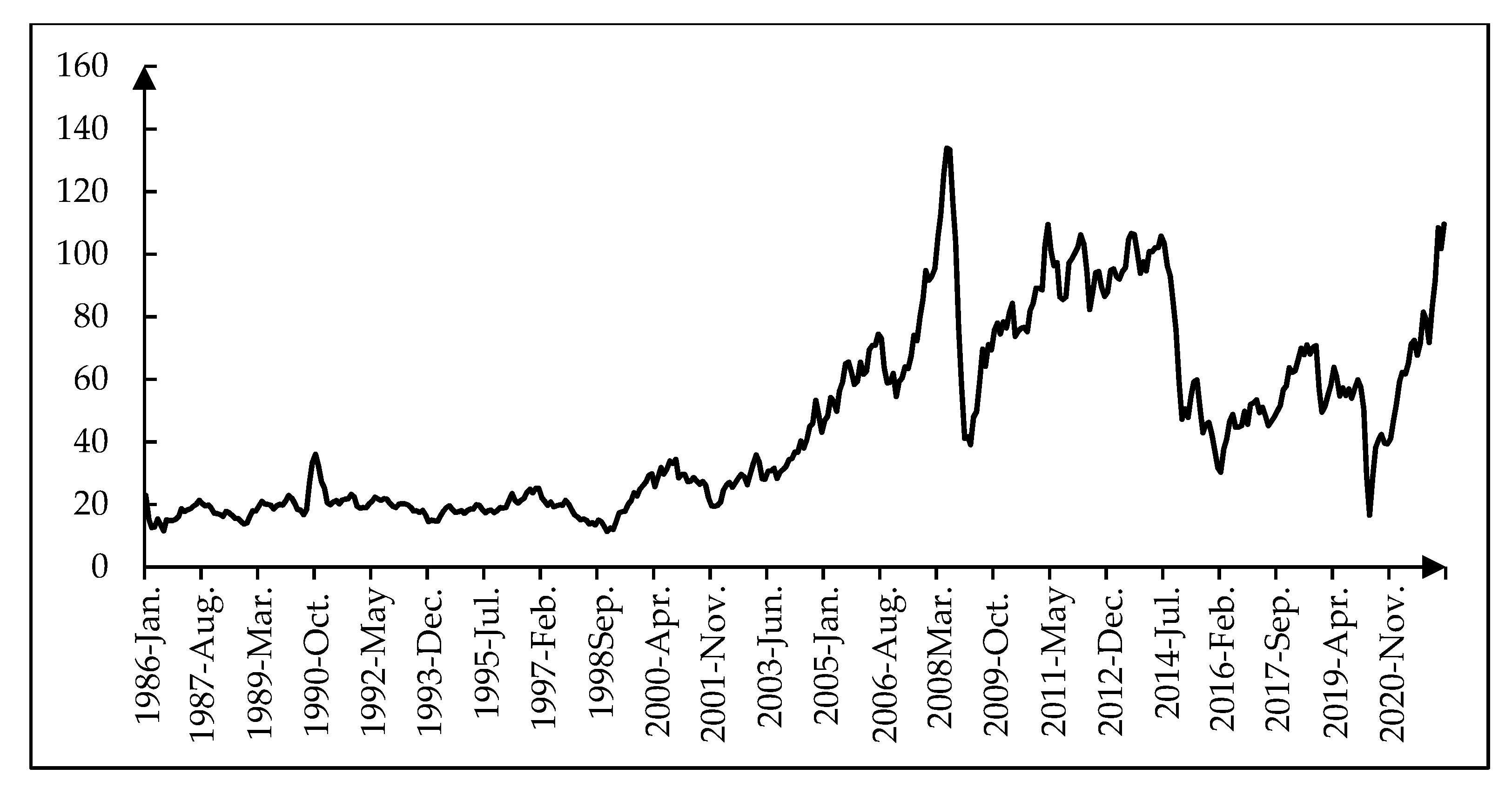
As is shown in Table 1, the main variables in this paper include: (1) Crude oil price (ROP). This variable is obtained based on the nominal international crude oil price and the US CPI index after deducting inflation. The nominal crude oil price mainly uses the spot price of crude oil of West Texas Intermediate (WTI), and the data are mainly from the website of the U.S. Energy Information Administration (EIA). We choose the WTI crude oil spot price as the index to measure the world oil price because WTI is one of the most important global oil markets. WTI crude oil spot price and Futures Crude oil price are the basic commodities of the oil futures contract of the New York Mercantile Exchange [36,37]. We choose the US CPI from January 1990 as the deflator to eliminate the influence of price factors. (2) VIX index (VIX). This variable is the real-time volatility index compiled by the Chicago Options Exchange (CBOE), which can measure the implied volatility of S&P 500 index options and is usually used to measure investors’ panic. The VIX index is expressed as an annualized percentage and can roughly reflect the expected trend of the S&P 500 index in the next 30 days. Therefore, a high VIX index indicates that investors believe that the market will fluctuate violently in the forward or reverse direction. The VIX index will be depressed only when investors believe that there is no great risk of decline and a possibility of rise. The data come from the wind database. (3) Return rate (RET). This variable is the monthly return series of the S&P 500 index. The change in the return series causes the change in the VIX index. The data come from the NASDAQ data link. (4) Global crude oil production (PRO). This reflects the impact of various political changes, wars and monopoly activities, which cause fluctuations in crude oil prices. The data come from the website of the U.S. Energy Information Administration (EIA). (5) Baltic dry bulk index (BDI). As the activity of global economic activities affects oil demand and leads to oil price volatility, the more prosperous the economy is, the stronger the driving force behind the oil price rise is. The variables used to measure global economic activities in this paper need to be monthly data and can reflect the changes in total global economic demand. Some studies use the weighting of industrial added value of all countries to measure the total demand of global economic activities, but there are two major problems: first, the industrial structure of many countries has changed greatly in the past decade, and the change in the proportion of industry in GDP leads to a change in energy intensity, so it is easy to produce the problem of sequence instability; second, it is difficult for each country to calculate its contribution to the global economy more and more accurately. Therefore, based on Kilian’s method, this paper uses the Baltic dry bulk index (BDI) as an index to measure the degree of global economic activity. The data come from the wind database. Since the earliest time for which we can obtain the WTI crude oil price is October 2002, considering the data collection, the sample period of the above variables is from October 2002 to November 2021, with a total of 229 observations.

Before constructing the time series model, we need to test the stationarity of each series and select the optimal lag order of the model. The results are shown in

Table 2. Unit root test.

Series	ADF Statistics	5% Critical Value	ADF Test Results
dlnrop	−11.43574 ***	−1.942224	Stable
dlnvix	−18.93658 ***	−2.874029	Stable
RET	−12.39050 ***	−3.429570	Stable
dlnpro	−14.60488 ***	−3.429657	Stable
dlnbdi	−13.77683 ***	−3.429657	Stable

Note: *** indicates significance at the level of 1%, and dlnrop, dlnvix, dlnpro and dlnbdi indicate log difference sequences of ROP, VIX, PRO and BDI, respectively.

and

Table 3. Determination of lag order.

Lag	AIC	SC	HQ
0	−5.948509	−5.902380	−5.929883
1	−6.428992	−6.244476 *	−6.354488 *
2	−6.466904 *	−6.144002	−6.336522
3	−6.464639	−6.003350	−6.278379
4	−6.446788	−5.847112	−6.204650
5	−6.428696	−5.690634	−6.130680

Note: * indicates the optimal lag order selected by the corresponding criteria.

. Specifically, we need to use the method of Dickey and Fuller [38] to test whether the unit root exists.

According to Table 2, the log difference sequence of ROP, VIX, PRO and BDI and the RET sequence are stable at the significance level of 1%. In order to avoid the problem of pseudo regression, the ADF unit root test is carried out on the studied sequences. It is found that the RET sequence is stable, while the ROP, VIX, PRO and BDI sequences are non-stationary. Therefore, the four sequences are processed by logarithmic difference, which is notated by dlnrop, dlnvix, dlnpro and dlnbdi. After processing, the ADF value of all sequences is less than the 5% critical value, which indicates that these sequences are stable; therefore, we can proceed to the next step of time series analysis.

According to Table 3, the optimal lag order of the TVP-VAR model is 1. Specifically, before constructing the TVP-VAR model, it is necessary to determine the optimal lag order of the model. As can be seen from Table 3, according to the minimum value criterion of AIC, the optimal lag order of the TVP-VAR model should be 2-lag with the minimum AIC value −6.446904, while according to the minimum value criterion of SC and HQ, the optimal lag order of the TVP-VAR model is 1-lag. Considering that the 1-lag order is selected by most criteria, we set the optimal lag order of our model to 1.

4. Empirical Results

4.1. The Time-Varying Dynamic Impact of Oil Price Volatility on Panic Index

MCMC simulation is used to estimate the parameters, and is set to conduct 10,000 MCMC simulations, of which the first 1000 are pre simulations. The specific estimation results of the model are shown in

Table 4. The estimation results of MCMC simulation parameter.

Parameter	Mean	STDEV	95%U	95%L	Geweke	Inef.
${\left({\mathsf{\Sigma }}_{\mathsf{\beta }}\right)}_1$	0.0224	0.0025	0.0181	0.0278	0.077	10.63
${\left({\mathsf{\Sigma }}_{\mathsf{\beta }}\right)}_2$	0.0227	0.0026	0.0183	0.0284	0.914	17.30
${\left({\mathsf{\Sigma }}_{\mathsf{\alpha }}\right)}_1$	0.0766	0.0272	0.0414	0.1514	0.755	84.33
${\left({\mathsf{\Sigma }}_{\mathsf{\alpha }}\right)}_2$	0.0515	0.0114	0.0338	0.0795	0.267	45.00
${\left({\mathsf{\Sigma }}_{\mathrm{h}}\right)}_1$	0.3877	0.0813	0.2480	0.5643	0.339	48.64
${\left({\mathsf{\Sigma }}_{\mathrm{h}}\right)}_2$	0.4124	0.1100	0.2172	0.6464	0.889	76.01

Note: Mean and STDEV, respectively, represent the mean and standard error of the posterior distribution of parameters, 95%U and 95%L, respectively, represent the upper and lower limits of the 95% confidence interval, Geweke represents the Geweke probability value, and Inef indicates an invalid influence factor.

.

Table 4 lists the parameter estimation results of the a posteriori distribution of MCMC simulation parameters. According to Geweke probability and invalid influence factor index results, we can judge that the MCMC simulation process is effective. At the significance level of 5%, the Geweke probability values are less than the critical value of 1.96, so the original assumption that “the estimated parameters converge to the a posteriori distribution” cannot be rejected. The maximum value of the invalid influence factor is 84.33, which means that MCMC estimates 10,000 samples and can obtain at least 118 (10,000/84.33) effective samples, indicating that the a posteriori mean is close to the real value of the parameters. Therefore, the MCMC simulation process is effective and robust, and the parameter estimation results are effective.

In this paper, the intervals of 1, 2 and 4 periods (lag of 1, 2 and 4 months) are selected to reflect the time-varying characteristics of the impulse response, so as to analyze the short-term, medium-term and long-term impact. The results are shown in Figure 3.

According to Figure 3, oil price volatility has a positive impact on VIX index, and this impact has time-varying characteristics. Firstly, in terms of the impact direction of different lag periods, except for a few years, the impact direction of short-term and medium-term crude oil price volatility is significantly positive, while the long-term impact effect is small. Specifically, as shown in Figure 3, except for a few years such as 2013–2014 and 2020–2021, the impact effect represented by the red line is significantly greater than 0 in other years, the impact effect represented by the blue line is significantly greater than 0 in almost all years, and the impact effect represented by the green line is close to 0. Secondly, from the comparison of impact intensity in different lag periods, the impact intensity of international crude oil price on the VIX index is the largest in lag period 2, followed by lag period 4 and lag period 6. Specifically, the red line in Figure 3 deviates from the zero axis more than the blue line, while the green line is close to the zero axis. This also shows that over time, the impact of oil price volatility on the panic index gradually weakened. Finally, from the trend of the impact effect of oil price volatility on the VIX index, the impact of oil price volatility on the VIX index varies in different periods. Specifically, the impact of international crude oil price on the VIX index since 2002 can be divided into three stages: the gentle period from the end of 2002 to 2006, the violent fluctuation period from 2007 to 2013, and the stable fluctuation period since 2014.

In addition, this paper also selects three time points before and after the subprime mortgage crisis (April 2007 and November 2008) and the period of negative oil price (April 2020) to analyze the impulse response relationship between oil price volatility and VIX index in different periods. Meanwhile, we selected the time point around April 2020 in consideration of the significant impact of the COVID-19 pandemic on oil price fluctuations, which are also the key topics of current academic research [39,40]. The results are shown in Figure 4.

According to Figure 4, the oil price volatility at different time points has a positive lagged impact on VIX index, but the impulse effects are different in convergence speed and intensity. Additionally, the impact path of oil price volatility on VIX index is relatively consistent, which starts to decline after the first period and tends to zero around the sixth period, but the convergence speed in April 2020 is faster. In terms of impact direction, it is significantly positive at the three time points when it lags behind one phase or two phases. In terms of impact intensity, the impact of crude oil prices in April 2007 and November 2008 is basically the same. In the current period and the first lag period, the impact intensity is lower than that in April 2020. This shows that initially, the impacts of oil price volatility in the period of financial crisis and COVID-19 are high, but are reduced rapidly, and the impacts of the COVID-19 pandemic on the VIX index last for about 3 months.

4.2. Heterogeneous Impacts of Oil Price Volatility from Different Sources on Panic Index

We use the SVAR model to decompose oil price volatility into demand shocks, supply shocks, and oil-specific demand shocks. The results are shown in Figure 5. At the top are described the impacts of crude oil supply shocks, in the middle are described the impacts of total oil demand shocks, and at the bottom are described the impacts of oil-specific demand shocks.

Figure 5 shows that the structural shocks of crude oil change with the passage of time. The impacts of oil price volatility in 2008 and 2020 are the largest, which is reflected in the impact fluctuation caused by total crude oil demand in 2008 and specific demand and supply in 2020. In 2008, the spread of the financial crisis greatly affected the real economy. From October to December 2008, the total demand for crude oil decreased sharply, with the result of a sharp decline in oil prices. In this period of abnormal oil price volatility, the impact of total economic demand was the leading factor. The abnormal fluctuation in oil price in 2020 is reflected in the impact of supply shock. In March and April 2020, OPEC fought a price war. Russia took the lead by increasing production and reducing prices to seize market share, resulting in a sharp increase in global crude oil supply and a sharp rise in international oil inventories, which was nearly 400 million barrels higher than the five-year average at the highest point. The international crude oil market showed an all-round surplus never before seen in history, resulting in a sharp decline in oil prices until OPEC implemented a new production reduction agreement in May 2020. It is clear that supply shocks are the underlying cause for the decline in oil prices in 2020.

Furthermore, we can calculate the contribution of supply shocks, total demand shocks and oil-specific demand shocks to oil price volatility by using the variance decomposition method. The results are shown in

Table 5. Variance decomposition result of oil price volatility (%).

Period	Supply Shocks	Aggregate Demand Shocks	Oil-Specific Demand Shocks
1	9.332167	0.682729	89.98510
2	9.658759	2.453038	87.88820
3	9.691828	4.178345	86.12983
4	9.662450	4.218357	86.11919
5	9.669220	4.254008	86.07677
6	9.672937	4.271717	86.05535
7	9.672941	4.273956	86.05310
8	9.672811	4.273881	86.05331
9	9.672843	4.274012	86.05315
10	9.672854	4.274083	86.05306

Note: The third to fifth columns in the table show the contribution rates of supply shocks, aggregate demand shock and oil-specific demand shocks to oil price volatility, respectively.

.

It can be seen from Table 5 that there are different contributions made by the three shocks. The largest contribution to the oil price volatility is the specific demand shock of crude oil, followed by the supply shock, and the total economic demand shock has the lowest contribution. Specifically, Table 5 also shows that as the number of lag periods increases, the contribution of supply shocks gradually decreases from 14.79% to 13.78%, but generally speaking, the decline is small, being only about 1%. The contribution of the impact of total economic demand has an upward trend, which gradually increases from 0.51% to about 6.00%. The contribution of specific demand shocks gradually decreased from 84.69% to 80.22, a decrease of 4.47%. All of these changes show that over time, the impact of total economic demand on oil price volatility gradually rises, while the impact of supply shock and specific demand shock on the original same price fluctuation continues to decline, which also affirms the importance of total economic demand.

This paper uses the polynomial distributed lag (PDL) model to analyze the impact of three structural shocks. Before regression analysis, we need to use the correlation coefficient matrix to judge whether there exists multicollinearity. By calculating the correlation coefficient matrix of the three structural residuals, it is found that the correlation coefficients between crude oil supply shocks and economic demand shocks is −0.0139; The correlation between crude oil supply shocks and oil-specific demand shocks is −0.0385, and the correlation coefficient between economic aggregate demand and specific demand shock is 0.0768, which shows that the three structural residuals can be put into the equation as explanatory variables at the same time. By using the PDL model, we can obtain the regression coefficients of the main explanatory variables. In order to more intuitively display the time-varying characteristics of the regression coefficient, we draw the coefficient with a broken line diagram, and the results are shown in Figure 6.

According to Figure 6, the effects of the three structural shocks on the VIX index are different. Specifically, from the perspective of the total effect of shocks, the impacts of oil price volatility from oil-specific demand shocks are generally positive, and the impacts of oil price volatility from crude oil supply shock and demand shock are generally negative (by summing up the shocks in each period, it can be concluded that the total coefficient of supply shocks is 1.634, the total coefficient of total demand shocks is −0.087, and the total coefficient of oil-specific demand shocks is 0.489). As for the time-varying characteristics of the impulse shocks, the impacts from oil supply shocks and oil-specific demand shocks show the transformation characteristics of “negative–positive”, while the impacts from total economic demand shocks show the transformation characteristics of “negative–positive”. Specifically, the impacts from supply shocks are positive in the current period and lag-one period, change to negative from the second period to sixth period, and turn to positive again in the seventh period. The impacts from total economic demand shocks are negative in the current period and the first three periods, and change to be positive after the fourth period. The impacts from oil-specific demand shocks are negative in the current period, change to positive in the first seven periods, and continue to be positive after a brief negative impact in the following four period. Moreover, we also find that the total impacts of the three structural shocks are negative only in the current period and the first five periods, and are all positive in other periods. From the perspective of impact intensity, the impacts from oil-specific demand shocks are the highest, followed by the supply shocks, and demand shocks. It is revealed by Figure 6 that the fluctuation range of the VIX index guided by oil-specific demand shocks is greater than that of supply shocks and total economic demand shocks. This is mainly because the oil-specific demand shocks of crude oil price cover all other factors except supply factors and demand factors, such as the expectations of market participants, financial speculation, oil inventory adjustment and other factors. This shows that the expectation of supply and demand factors and the impact caused by financial market speculation have raised oil prices and are more likely to cause market panic.

4.3. Asymmetric Impacts of Oil Price Volatility in Different Directions on Panic Index

Based on the decomposition results of oil price volatility, we use the TARCH model to estimate the asymmetric impact of oil price volatility caused by supply factors, demand factors and specific demand factors on VIX, respectively. The results are shown in

Table 6. The TARCH estimation result of oil price volatility from supply shock and VIX index.

Variable	Coefficient	Std. Error	z-Statistic	Prob.
$\mathsf{\omega }$	0.019781	0.004584	4.314955	0.0000
${\mathrm{u}}_{\mathrm{t}-1}^2$	0.552247	0.202405	2.728427	0.0064
${\mathrm{u}}_{\mathrm{t}-1}^2{\mathrm{d}}_{\mathrm{t}-1}$	−0.686433	0.218695	−3.138766	0.0017
${\mathsf{\sigma }}_{\mathrm{t}-1}^2$	0.280111	0.141793	1.975484	0.0482

,

Table 7. The TARCH estimation result of oil price volatility from aggregate demand shock and VIX index.

Variable	Coefficient	Std. Error	z-Statistic	Prob.
$\mathsf{\omega }$	0.017063	0.003965	4.303282	0.0000
${\mathrm{u}}_{\mathrm{t}-1}^2$	0.516161	0.177094	2.914622	0.0036
${\mathrm{u}}_{\mathrm{t}-1}^2{\mathrm{d}}_{\mathrm{t}-1}$	−0.682688	0.194532	−3.509378	0.0004
${\mathsf{\sigma }}_{\mathrm{t}-1}^2$	0.370813	0.134791	2.751032	0.0059

and

Table 8. The TARCH estimation result of oil price volatility from oil-specific demand shock and VIX index.

Variable	Coefficient	Std. Error	z-Statistic	Prob.
$\mathsf{\omega }$	0.017873	0.005385	3.319149	0.0009
${\mathrm{u}}_{\mathrm{t}-1}^2$	0.491074	0.175477	2.798510	0.0051
${\mathrm{u}}_{\mathrm{t}-1}^2{\mathrm{d}}_{\mathrm{t}-1}$	−0.599164	0.191262	−3.132677	0.0017
${\mathsf{\sigma }}_{\mathrm{t}-1}^2$	0.325901	0.184794	1.763589	0.0778

.

According to Table 6, Table 7 and Table 8, the structural oil price shock has an asymmetric effect on the panic index, that is, the positive structural oil price shock has a greater effect on the panic index than the negative structural oil price shock. Specifically, as shown in Table 6, the coefficient in front of the variable ${\mathrm{u}}_{\mathrm{t}-1}^2$ is 0.552247, while the coefficient in front of the variable ${\mathrm{u}}_{\mathrm{t}-1}^2{\mathrm{d}}_{\mathrm{t}-1}$ is −0.686433, which has passed the significance test of 1%. It shows that the asymmetric effect reduces the fluctuation range. When the supply shock increases, its effect coefficient on the panic index is 0.552247. When the supply shock decreases, its effect coefficient on the panic index is −0.134186 (0.552247–0.686433). As shown in Table 7, the coefficient in front of the variable ${\mathrm{u}}_{\mathrm{t}-1}^2$ is 0.516161, which passes the 1% significance test, while the coefficient in front of the variable ${\mathrm{u}}_{\mathrm{t}-1}^2{\mathrm{d}}_{\mathrm{t}-1}$ is −0.682688, which also passes the significance test of 1%. This also shows that the asymmetric effect will reduce the fluctuation range, and the action coefficient of the increase in demand shock is 0.540332 greater than that of the decrease in demand shock. As for Table 8, the coefficient in front of the variable ${\mathrm{u}}_{\mathrm{t}-1}^2$ is 0.491074, while the coefficient in front of the variable ${\mathrm{u}}_{\mathrm{t}-1}^2{\mathrm{d}}_{\mathrm{t}-1}$ is −0.626594, which passes the significance test of 1%. This also shows that the asymmetric effect reduces the fluctuation range. When the specific demand shock increases, its effect coefficient on the panic index is 0.491074. When the impact of specific demand decreases, its effect coefficient on the panic index is −0.10809 (0.491074–0.599164). From Table 6, Table 7 and Table 8, whether supply shock (Table 6) or oil-specific demand shock (Table 8), the coefficients in front of variables ${\mathrm{u}}_{\mathrm{t}-1}^2{\mathrm{d}}_{\mathrm{t}-1}$ are significantly negative, and it can be concluded that the impact of positive supply shock and specific demand shock on the panic index is greater than that of negative shock. This may be due to the fact that the driving effect of rapid economic development partially or completely offsets the inhibitory effect caused by the rise in oil prices. Therefore, the rise in oil prices driven by economic demand factors has a relatively small impact on the panic index; however, the impact of the rise in oil prices caused by oil-specific demand on investor sentiment can partly reflect that there is still speculation in the capital market. The rise in oil prices driven by supply factors is more likely to increase the uncertainty of market expectations for oil prices and lead to a rise in the panic index.

5. Discussion

Empirical results reveal that oil price volatility has an important influence on the VIX index. Prior studies were concerned more with the relationship between oil price volatility and the stock market. Most of these studies found that the stock market is highly related to oil price volatility [4,15,16,17,18,19,20,21,41]. However, only few studies address the oil price volatility and VIX index, and the uncertainty of the relationship between them. For example, Choi and Hong [42] found that the OVX and VIX show bi-directional causality during shale gas revolution by using the ARDL model and the Granger causality tests. However, the research of Liu et al. [43] shows that there are only significant short-run relationships between crude oil volatility and VIX index, rather than long-run equilibrium relationships. Differently from these studies, we use the TVP-VAR model to examine the time-varying impacts. Additionally, the TVP-VAR model was used by Corbet et al. [44] to explore the dynamic connectedness between WTI oil and other US energy prices. Regarding the SVAR model, Kilian [22] found that compared with supply shock, the rise in oil price caused by demand shock has a greater impact on US GDP and inflation. In our study, we find that the impacts of oil price volatility from oil-specific demand shocks are greater than those of oil supply shocks and demand shocks. Moreover, similar to the research of Onan, Salih and Yasar [30], the asymmetric effects are explored. We conclude that the positive oil price shock has a greater effect on the VIX index than the negative oil price shock. Although oil prices may cause investors’ panic, it is worth mentioning that frontier technologies such as blockchain technology may bring new changes to the crude oil market [41,42,43,44,45]. When studying the impact of international crude oil prices on the market, we may need to examine the moderator role of frontier technologies. This is our future research direction. In addition, crude oil not only has financial attributes, but also commodity attributes. This paper studies the impact of crude oil price fluctuation on the panic index, which emphasizes its financial attributes more than its commodity attributes. In fact, the impact of crude oil price fluctuations on investor sentiment is also reflected in consumer markets (automobile gasoline prices), enterprises (such as chemical enterprises), and other market participants. This is also worthy of study.

In order to effectively respond to the impacts of oil price volatility, governments need to adopt different coping strategies for oil price rises according to different oil price shock sources: (1) From the supply perspective, countries should put an emphasis on oil security, actively respond to changes in the international oil market and construct a diversified oil supply system. (2) From the demand perspective, the rise in crude oil demand leads to the rise in oil price, which has a certain output expansion effect on the domestic industrial sector. However, the situation of highly relying on investment and export is not conducive to sustainable economic development. On the one hand, countries need to change their mode of economic growth, reduce the proportion of fossil energy, control energy consumption, and improve energy efficiency. On the other hand, they need to strengthen energy supply capacity and develop clean and renewable energy. In addition, it is thought that blockchain technology can provide a secure and immutable ledger of value transfers in a network, which will facilitate the replacement of crude oil by renewable energy. Additionally, similar to bitcoin [46], different financial assets’ volatility may affect each other. Oil price volatility may affect other financial markets. Promoting the marketization of energy pricing or trading may also be conducive to reducing the adverse impact of oil price volatility. For example, some scholars, such as Chantrel, Surmann, Erge and Thomsen [41], Yapa, de Alwis, Liyanage and Ekanayake [42], Kirli, Couraud, Robu, Salgado-Bravo, Norbu, Andoni, Antonopoulos, Negrete-Pincetic, Flynn and Kiprakis [43], and Górski [44] proposed blockchain technology for renewable energy trading. (3) From the oil-specific demand perspective, the derivatives market based on oil and other bulk commodities is developing rapidly. Enterprises can use derivatives trading to avoid the adverse impact of oil price changes. Therefore, countries should expand the crude oil futures market and provide more convenient risk-hedging tools for the activities relevant to crude oil production.

6. Conclusions

Crude oil is the essential raw material for modern industrial production, and its price volatility penetrates all aspects of the development of the real economy along the industrial value chain. Meanwhile, crude oil also has the attribute of financial assets, which causes the impacts of oil price volatility on the real economy to gradually spread to the capital market. This paper uses the VIX index to measure the panic in the capital market, collects the time series data of WTI crude oil price and the VIX index, and analyzes the time-varying, heterogeneous and asymmetric impact of oil price volatility on the VIX index. The main conclusions are as follows: Firstly, we use the TVP-VAR model to analyze the time-varying impact of oil price volatility on the VIX index. The results show that oil price volatility can significantly affect the VIX index, and this impact has time-varying characteristics. Then, using Kilian’s method and the SVAR model, we decompose the oil price volatility into three factors: demand factor, supply factor and specific demand factor. Then, we use the PDL model to investigate the heterogeneous impact of oil price volatility from different sources on the VIX index. The results show that the oil price volatility from different sources has different impacts on the panic index, and the order from high to low is oil-specific demand shocks, supply shocks, and total aggregate shocks. Finally, we use the decomposition results of crude oil price and use the TARCH model to investigate the asymmetric impacts of oil price volatility in different directions on the panic index. The results show that oil price volatility in different directions has asymmetric impacts on the VIX index, and the impact of positive oil price shock is greater than that of the negative.

In order to effectively respond to the impacts of oil price volatility, governments need to adopt different coping strategies for oil price rises according to different oil price shock sources: (1) From the supply perspective, countries should put an emphasis on oil security, actively respond to changes in the international oil market and construct a diversified oil supply system. (2) From the demand perspective, the rise in crude oil demand leads to the rise in oil price, which has a certain output expansion effect on the domestic industrial sector. However, the situation of highly relying on investment and export is not conducive to sustainable economic development. On the one hand, countries need to change their mode of economic growth, reduce the proportion of fossil energy, control energy consumption, and improve energy efficiency. On the other hand, they need to strengthen energy supply capacity and develop clean and renewable energy. In addition, promoting the marketization of energy pricing or trading is also conducive to reducing the adverse impact of oil price volatility. For example, some scholars, such as Chantrel et al. [41], Yapa et al. [42], Kirli et al. [43], and Górski [44], proposed blockchain technology for renewable energy trading. It is thought that blockchain technology can provide a secure and immutable ledger of value transfers in a network, which will facilitate the replacement of crude oil by renewable energy. (3) From the oil-specific demand perspective, the derivatives market based on oil and other bulk commodities is developing rapidly. Enterprises can use derivatives trading to avoid the adverse impact of oil price changes. Therefore, countries should expand the crude oil futures market and provide more convenient risk-hedging tools for the activities relevant to crude oil production.

References

1. Moghaddam, M.B.; Lloyd-Ellis, H. Heterogeneous effects of oil price fluctuations: Evidence from a nonparametric panel data model in Canada. Energy Econ. 2022, 110, 106012. [Google Scholar] [CrossRef]
2. Liu, Y.; Sharma, P.; Jain, V.; Shukla, A.; Shahzad Shabbir, M.; Tabash, M.I.; Chawla, C. The relationship among oil prices volatility, inflation rate, and sustainable economic growth: Evidence from top oil importer and exporter countries. Resour. Policy 2022, 77, 102674. [Google Scholar] [CrossRef]
3. Huang, J.; Dong, X.; Chen, J.; Zhong, M. Do oil prices and economic policy uncertainty matter for precious metal returns? New insights from a TVP-VAR framework. Int. Rev. Econ. Financ. 2022, 78, 433–445. [Google Scholar] [CrossRef]
4. Li, Z.; Ao, Z.; Mo, B. Revisiting the Valuable Roles of Global Financial Assets for International Stock Markets: Quantile Coherence and Causality-in-Quantiles Approaches. Mathematics 2021, 9, 1750. [Google Scholar] [CrossRef]
5. Li, F.; Yang, C.; Li, Z.; Failler, P. Does Geopolitics Have an Impact on Energy Trade? Empirical Research on Emerging Countries. Sustainability 2021, 13, 5199. [Google Scholar] [CrossRef]
6. Ding, Z.; Liu, Z.; Zhang, Y.; Long, R. The contagion effect of international crude oil price fluctuations on Chinese stock market investor sentiment. Appl. Energy 2017, 187, 27–36. [Google Scholar] [CrossRef]
7. Herrera, A.M.; Karaki, M.B.; Rangaraju, S.K. Oil price shocks and U.S. economic activity. Energy Policy 2019, 129, 89–99. [Google Scholar] [CrossRef]
8. Sek, S.K. Impact of oil price changes on domestic price inflation at disaggregated levels_ Evidence from linear and nonlinear ARDL modeling. Energy 2017, 130, 204–217. [Google Scholar] [CrossRef]
9. Zhu, H.; Chen, X. Asymmetric effects of oil prices and exchange rates on China’s industrial prices. Energy Econ. 2019, 84, 104551. [Google Scholar] [CrossRef]
10. Dedeoğlu, D.; Kaya, H. Pass-through of oil prices to domestic prices: Evidence from an oil-hungry but oil-poor emerging market. Econ. Model. 2014, 43, 67–74. [Google Scholar] [CrossRef]
11. Chen, J.; Zhu, X.; Li, H. The pass-through effects of oil price shocks on China’s inflation: A time-varying analysis. Energy Econ. 2020, 86, 104695. [Google Scholar] [CrossRef]
12. Huang, W.-H.; Chao, M.-C. The effects of oil prices on the price indices in Taiwan. Energy Policy 2012, 45, 730–738. [Google Scholar] [CrossRef]
13. Özdurak, C. Nexus between crude oil prices, clean energy investments, technology companies and energy democracy. Green Financ. 2021, 3, 337–350. [Google Scholar] [CrossRef]
14. Sazzad Jeris, S.; Deb Nath, R. COVID-19, oil price and UK economic policy uncertainty: Evidence from the ARDL approach. Quant. Financ. Econ. 2020, 4, 503–514. [Google Scholar] [CrossRef]
15. Joo, Y.C.; Park, S.Y. The impact of oil price volatility on stock markets: Evidences from oil-importing countries. Energy Econ. 2021, 101, 105413. [Google Scholar] [CrossRef]
16. Cheema, M.A.; Scrimgeour, F. Oil prices and stock market anomalies. Energy Econ. 2019, 83, 578–587. [Google Scholar] [CrossRef] [Green Version]
17. Wei, Y.; Guo, X. Oil price shocks and China’s stock market. Energy 2017, 140, 185–197. [Google Scholar] [CrossRef]
18. Hwang, I.; Kim, J. Oil price shocks and the US stock market: A nonlinear approach. J. Empir. Financ. 2021, 64, 23–36. [Google Scholar] [CrossRef]
19. Wang, Y.; Wu, C.; Yang, L. Oil price shocks and stock market activities: Evidence from oil-importing and oil-exporting countries. J. Comp. Econ. 2013, 41, 1220–1239. [Google Scholar] [CrossRef]
20. Kang, W.; Ratti, R.A.; Yoon, K.H. Time-varying effect of oil market shocks on the stock market. J. Bank. Financ. 2015, 61, S150–S163. [Google Scholar] [CrossRef] [Green Version]
21. Smyth, R.; Narayan, P.K. What do we know about oil prices and stock returns? Int. Rev. Financ. Anal. 2018, 57, 148–156. [Google Scholar] [CrossRef]
22. Kilian, L. Not All Oil Price Shocks Are Alike: Disentangling Demand and Supply Shocks in the Crude Oil Market. Am. Econ. Rev. 2009, 99, 1053–1069. [Google Scholar] [CrossRef] [Green Version]
23. Lippi, F.; Nobili, A. Oil and the Macroeconomy: A Quantitative Structural Analysis. J. Eur. Econ. Assoc. 2012, 10, 1059–1083. [Google Scholar] [CrossRef] [Green Version]
24. Bastianin, A.; Conti, F.; Manera, M. The impacts of oil price shocks on stock market volatility: Evidence from the G7 countries. Energy Policy 2016, 98, 160–169. [Google Scholar] [CrossRef]
25. Cunado, J.; Perez de Gracia, F. Oil price shocks and stock market returns: Evidence for some European countries. Energy Econ. 2014, 42, 365–377. [Google Scholar] [CrossRef]
26. Nikkinen, J.; Sahlström, P. Impact of the federal open market committee’s meetings and scheduled macroeconomic news on stock market uncertainty. Int. Rev. Financ. Anal. 2004, 13, 1–12. [Google Scholar] [CrossRef]
27. Chen, E.-T.; Clements, A. S&P 500 implied volatility and monetary policy announcements. Financ. Res. Lett. 2007, 4, 227–232. [Google Scholar] [CrossRef]
28. Krieger, K.; Mauck, N.; Vazquez, J. Comparing U.S. and European market volatility responses to interest rate policy announcements. Int. Rev. Financ. Anal. 2015, 39, 127–136. [Google Scholar] [CrossRef] [Green Version]
29. Fernandez-Perez, A.; Frijns, B.; Tourani-Rad, A. When no news is good news—The decrease in investor fear after the FOMC announcement. J. Empir. Financ. 2017, 41, 187–199. [Google Scholar] [CrossRef] [Green Version]
30. Onan, M.; Salih, A.; Yasar, B. Impact of macroeconomic announcements on implied volatility slope of SPX options and VIX. Financ. Res. Lett. 2014, 11, 454–462. [Google Scholar] [CrossRef] [Green Version]
31. Primiceri, G.E. Time Varying Structural Vector Autoregressions and Monetary Policy. Rev. Econ. Stud. 2005, 72, 821–852. [Google Scholar] [CrossRef]
32. Nakajima, J.; Kasuya, M.; Watanabe, T. Bayesian analysis of time-varying parameter vector autoregressive model for the Japanese economy and monetary policy. J. Jpn. Int. Econ. 2011, 25, 225–245. [Google Scholar] [CrossRef] [Green Version]
33. Feng, Y.; Chen, S.; Xuan, W.; Yong, T. Time-varying impact of U.S. financial conditions on China’s inflation: A perspective of different types of events. Quant. Financ. Econ. 2021, 5, 604–622. [Google Scholar] [CrossRef]
34. Bekiros, S.D.; Diks, C.G.H. The relationship between crude oil spot and futures prices: Cointegration, linear and nonlinear causality. Energy Econ. 2008, 30, 2673–2685. [Google Scholar] [CrossRef] [Green Version]
35. Nonejad, N. Should crude oil price volatility receive more attention than the price of crude oil? An empirical investigation via a large-scale out-of-sample forecast evaluation of US macroeconomic data. J. Forecast. 2020, 40, 769–791. [Google Scholar] [CrossRef]
36. Dickey, D.A.; Fuller, W.A. Distribution of the Estimators for Autoregressive Time Series With a Unit Root. J. Am. Stat. Assoc. 1979, 74, 427–431. [Google Scholar] [CrossRef]
37. Awan, T.M.; Khan, M.S.; Haq, I.U.; Kazmi, S. Oil and stock markets volatility during pandemic times: A review of G7 countries. Green Financ. 2021, 3, 15–27. [Google Scholar] [CrossRef]
38. Wu, Y.; Ma, S. Impact of COVID-19 on energy prices and main macroeconomic indicators—Evidence from China’s energy market. Green Financ. 2021, 3, 383–402. [Google Scholar] [CrossRef]
39. Glosten, L.R.; Jagannathan, R.; Runkle, D.E. On the Relation between the Expected Value and the Volatility of the Nominal Excess Return on Stocks. J. Financ. 1993, 48, 1779–1801. [Google Scholar] [CrossRef]
40. Zakoian, J.-M. Threshold heteroskedastic models. J. Econ. Dyn. Control 1994, 18, 931–955. [Google Scholar] [CrossRef]
41. Chantrel, S.P.M.; Surmann, A.; Erge, T.; Thomsen, J. Participative Renewable Energy Community—How Blockchain-Based Governance Enables a German Interpretation of RED II. Electricity 2021, 2, 471–486. [Google Scholar] [CrossRef]
42. Yapa, C.; de Alwis, C.; Liyanage, M.; Ekanayake, J. Survey on blockchain for future smart grids: Technical aspects, applications, integration challenges and future research. Energy Rep. 2021, 7, 6530–6564. [Google Scholar] [CrossRef]
43. Kirli, D.; Couraud, B.; Robu, V.; Salgado-Bravo, M.; Norbu, S.; Andoni, M.; Antonopoulos, I.; Negrete-Pincetic, M.; Flynn, D.; Kiprakis, A. Smart contracts in energy systems: A systematic review of fundamental approaches and implementations. Renew. Sustain. Energy Rev. 2022, 158, 112013. [Google Scholar] [CrossRef]
44. Górski, T. Reconfigurable Smart Contracts for Renewable Energy Exchange with Re-Use of Verification Rules. Appl. Sci. 2022, 12, 5339. [Google Scholar] [CrossRef]
45. Son, Y.-B.; Im, J.-H.; Kwon, H.-Y.; Jeon, S.-Y.; Lee, M.-K. Privacy-Preserving Peer-to-Peer Energy Trading in Blockchain-Enabled Smart Grids Using Functional Encryption. Energies 2020, 13, 1321. [Google Scholar] [CrossRef] [Green Version]
46. Li, Z.; Dong, H.; Floros, C.; Charemis, A.; Failler, P. Re-examining Bitcoin Volatility: A CAViaR-based Approach. Emerg. Mark. Financ. Trade 2021, 58, 1320–1338. [Google Scholar] [CrossRef]
Figure 1. The WTI spot price (source: https://www.eia.gov/dnav/pet/pet_pri_spt_s1_d.htm (accessed on 23 June 2022)).
Energies 15 04629 g001
Figure 2. Framework diagram.
Energies 15 04629 g002
Figure 3. Impulse response of VIX index to international crude oil price in different periods.
Energies 15 04629 g003
Figure 4. Impulse response of VIX index to crude oil price at different time points.
Energies 15 04629 g004
Figure 5. Structural shock based on the decomposition of oil price volatility.
Energies 15 04629 g005
Figure 6. Changes in parameters of VIX index in response to structural shock.
Energies 15 04629 g006