Article

Finite Element Method for Non-Newtonian Radiative Maxwell Nanofluid Flow under the Influence of Heat and Mass Transfer

1
Department of Mathematics, Air University, PAF Complex E-9, Islamabad 44000, Pakistan
2
Department of Mathematics and Sciences, College of Humanities and Sciences, Prince Sultan University, Riyadh 11586, Saudi Arabia
3
Stochastic Analysis and Optimization Research Group, Department of Mathematics, Air University, PAF Complex E-9, Islamabad 44000, Pakistan
4
Department of Mathematics, Comsats University Islamabad, Islamabad 44000, Pakistan
*
Author to whom correspondence should be addressed.
Energies 2022, 15(13), 4713; https://doi.org/10.3390/en15134713
Submission received: 27 May 2022 / Revised: 16 June 2022 / Accepted: 22 June 2022 / Published: 27 June 2022
(This article belongs to the Special Issue Computational Fluid Flow, Heat Transfer and Energy Impacts)

Abstract

:
The recent study was concerned with employing the finite element method for heat and mass transfer of MHD Maxwell nanofluid flow over the stretching sheet under the effects of radiations and chemical reactions. Moreover, the effects of viscous dissipation and porous plate were considered. The mathematical model of the flow was described in the form of a set of partial differential equations (PDEs). Further, these PDEs were transformed into a set of nonlinear ordinary differential equations (ODEs) using similarity transformations. Rather than analytical integrations, numerical integration was used to compute integrals obtained by applying the finite element method. The mesh-free analysis and comparison of the finite element method with the finite difference method are also provided to justify the calculated results. The effect of different parameters on velocity, temperature and concentration profile is shown in graphs, and numerical values for physical quantities of interest are also given in a tabular form. In addition, simulations were carried out by employing software that applies the finite element method for solving PDEs. The calculated results are also portrayed in graphs with varying sheet velocities. The results show that the second-order finite difference method is more accurate than the finite element method with linear interpolation polynomial. However, the finite element method requires less number of iterations than the finite difference method in a considered particular case. We had high hopes that this work would act as a roadmap for future researchers entrusted with resolving outstanding challenges in the realm of enclosures utilized in industry and engineering.

1. Introduction

The extensive manufacturing and industrial applications have made studying boundary layer non-Newtonian fluid much more substantial for the research scholars. Several processes such as reparating plastic polymers, hot rolling, cooling metallic plates, drilling muds and assembling optical fibers have followed the principles of boundary layer non-Newtonian fluid. Scientists have suggested integral and rate models for boundary layer studies as a single model is not enough to cover the versatility of properties. The given study comprises the Maxwell fluid model, which is the subclass of the rate type model and is used to determine the effect of relaxation time.
The most stimulating area in applied sciences is the non-Newtonian fluid flow, which has attracted many scholars due to its extensive medical and engineering applications (Rivlin and Ericksen [1]). This fluid exhibits several alternating properties such as variable rheological parameters and a non-singular constitutive equation, making it unreliable. Therefore, scientists have suggested different models, (i) differential type, (ii) rate type and (iii) integral type [2,3], to well fathom med the non-Newtonian fluid flow. Maxwell fluid is the liquid that depicts qualities such as improved elasticity and viscosity [4,5], making it more enigmatic in fluid dynamics. The Maxwell fluid model is the subclass of rate type fluid model and can anticipate stress relaxation. Generalization of Maxwell material is the Upper Convected Maxwell (UCM) model for the case of large deformation using the upper convected time derivative.
Initially, Maxwell investigated the viscoelastic effect of air [6], which Mukhopadhyay and Bhattacharyya [7] extended by examining an uneven Maxwell fluid flow study across a stretching sheet with a chemical reaction. Nadeem and his colleagues later discovered the viscoelastic fluid flow influenced by the Cattaneo–Christov theory and Newtonian heating across an exponentially stretched sheet. Further modification to [8] was performed in Nadeem et al. [9] by introducing thermal stratification to the boundary layer flow of Maxwell fluid using the Cattaneo–Christov theory. Some exponential work was conducted by khan et al. [10]. His work was profound due to the slip conditions applied to stretching sheets with mas transfer and chemically active Maxwell fluid. Details related to boundary layer flow can be traced [11,12].
Extensive research on the MHD fluid flow results from its excessive industrial applications that fascinated several research scholars [13,14,15,16]. During the last few decades, MHD flow through parallel channels gained the focus of many scientists. Ref. [17] was the first who prepared the homotopy analysis method (HAM) and investigated the MHD flow of an upper convected Maxwell (UCM) fluid using a porous stretching sheet. Raftari and Yildirim [18] modified the work conducted by Hayat et al. [17] and invented a novel technique model referred to as a homotopy perturbation method (HPM). Sajid et al. [19] proposed a rotating flow instead of a non-rotating one. They purposely estimated the improved performance of UCM due to the rotation parameter, which controlled the boundary layer’s thickness, hence advancing the study. Comparatively, the analytical studies are given by Hayat et al. [17] and Raftari and Yildirim [18]. MHD flow across a stretching sheet was studied by Abel et al. [20] using the fourth-order Runge–Kutta method. The findings of the above studies were confined to the no-slip boundary condition imposed along with the flat plate, which was further improved by Abbasi and Rahimipetroudi [21], who considered the slip boundary condition of a UCM Maxwell fluid via HPM. Nadeem et al. [22] added dimensions to the Maxwell fluid model that enhanced the complexity and efficiency of a Maxwell fluid’s MHD boundary layer flow with nanoparticles. Moreover, Afify and Elgazery [23] introduced a chemical reaction into their model, extending the Nadeem et al. [22] study.
The magnetic field now removes non-metallic substances from molten metals, purifying metals from non-metallic turbidity. In this regard, magnetohydrodynamic fluid has a separate fan base as it is used in several industrial procedures, such as extracting metals from their ores and removing petrol from their reservoirs. Electrically conductive fluids are used in power generators, cancer treatment, MRI, heat exchangers and many more applications. When investigating non-Newtonian fluid flow, Sarpakaya [24] is regarded as a pioneer. Turkyilmazoglu [25] suggested extending this work by inoculating variable viscosity and studying the turbulent convective MHD fluid flow.
Turkyilmazoglu [26] discovered different solutions for two types of viscoelastic fluid using MHD slip flow across the stretching surface. Dhanai et al. [27] investigated Sisko nanofluid and applied variable MHD flow and energy transfer solutions combined with convective boundary conditions. Ellahi et al. [28] examine Hall’s current MHD Jeffrey fluid flow effect. He prepared his study on the rectangular duct. Ahmad and Nadeem introduced the introduction of nanotubes to MHD fluid flow [29] with the combined effect of Cattaneo–Christov heat flux theory. A similar flow was examined by Farooq et al. [30]. The researcher studied an MHD flow of Maxwell fluid via a nanomaterial stretched surface. Details of MHD flow of Carreau fluid based on Cattaneo–Christov flux theory can easily be spotted in [31,32].
A new focus on mass heat flow has brought experts together, and they discovered that it could be used in a wide range of fields such as air conditioning, electronic device cooling and nuclear reactor cooling. It can also be used to desalinate water and in the food and pharmaceutical industries. Initially, the Fourier [33] and Fick [34] laws were used for interpreting mass and heat flow best, but later on, scientists observed some limitations of these laws, which could affect the studies. One of the most scavenging drawbacks is forming a parabolic type of equation. Javed and Nadeem [35] utilized two concentric cylinders to observe Casson fluid’s mass and energy flow. Double stratified second-grade fluid flow was studied by Mallawi and colleagues [36] using the Riga plate heat flux model and thermal radiation. A review of the literature [37,38] revealed the focus of various scholars on heat transfer of turbulent nanofluid flow to minimize the energy consumption in a solar collector.
The study of Darcy–Forchheimer flow of Reiner–Philippoff nanofluid over the stretching sheet was investigated in [39] with the involvement of Motile microorganisms. The effects of heat source/sink and melting phenomenon were also considered. The Matlab solver was considered to solve the obtained dimensionless equations. The results confirmed that rising thermophoresis and Schmidt number values enhanced the heat transfer coefficient. By changing thermophysical characteristics, entropy reduction in the thermos and non-Newtonian nanofluid models was addressed [40]. Two types of nanofluids, namely Copper–Engine Oil and Zinconium Dioxide–Engine Oil, were considered for the study. The effects of different parameters on velocity, temperature and entropy distribution are shown in graphs. The Keller–Box scheme was implemented to solve differential equations obtained from the fluid phenomenon. A mixture model was considered to simulate a rotating tube bundle [41]. The microchannel heat exchanger’s performance was assessed by applying various operating factors such as Reynolds number, rotation speed and concentration of the nanofluid. Instead of finding numerical solutions, exact expressions for dimensionless velocity and temperature were obtained in [42]. It was pointed out that the Newtonian fluid flow was faster than Maxwell fluid flow.
Since the finite element method is one of the numerical methods that can be used to find the solutions to linear and nonlinear ordinary and partial differential equations, the recent approach to applying the method is based on Galerkin weighted residuals, and integrals in this approach are computed using numerical Gauss–Legendre three points formula integrations. The model for non-Newtonian fluid flow over stretching sheet is given, and converted ODEs were solved by applying three numerical approaches. The second applied method is the finite difference method, which is second-order accurate at all the grid points except the last one. The numerical experiments conclude that the finite difference method (FDM) is more accurate than the finite element method (FEM) with linear interpolation polynomial for the considered problem.
Moreover, a Matlab solver bvp4c was also employed for solving nonlinear dimensionless ODEs. The solver can be used to find solutions to problems in finite domains. Even though the domain of the considered problem is infinite, a finite domain is chosen for numerical purposes. The solver, in most cases, converges, but it may give an error. As a result, an additional loop is utilized to make the procedure workable for some or all of the cases of the problem under consideration.

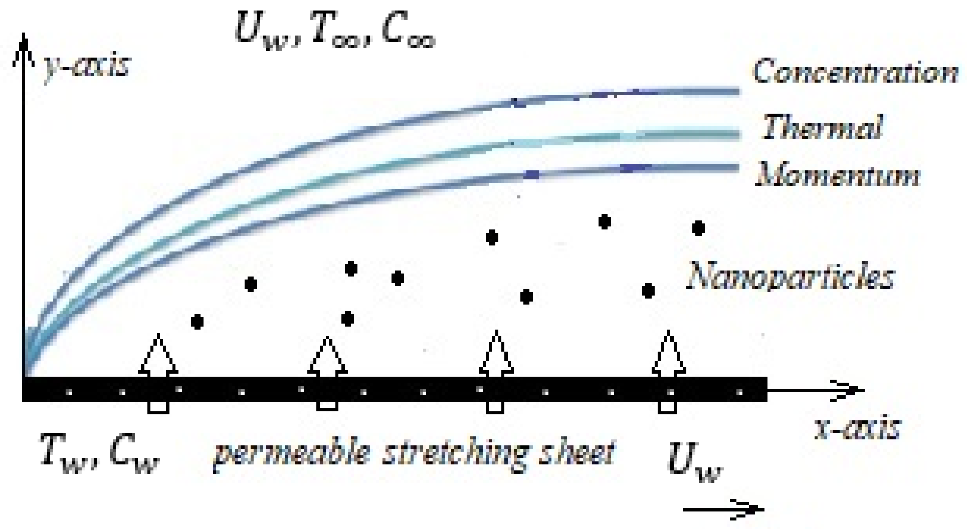
2. Problem Formulation

Consider incompressible, laminar, steady, electrically conductive two-dimensional non-Newtonian Maxwell nanofluid flow over a stretching sheet. Let the plate be stretched with stretching velocity U W . Let x -axis be taken along the sheet and y -axis be taken perpendicular to the sheet. The flow is generated by the sudden movement of the sheet towards the positive x -axis. The fluid is embedded in a porous medium, and the permeability of this porous medium is denoted by k . The magnetic field has strength B 0 applied perpendicular to the sheet. Let u and v be the velocity components in x and y directions, respectively. The fluid temperature is denoted by T , and concentration is denoted by C . Let T w and C w be temperature and concentration at the plate, whereas T and C is the temperature and concentration away from the plate. Under the boundary layer assumption(s), the governing equations of this phenomenon can be expressed as:
u x + v y   = 0
u u x + v u y + λ 0 u 2 2 u x 2 + v 2 2 u y 2 + 2 u v 2 u x y = ν 2 u y 2 ν k u σ B 0 2 ρ u
u T x + v T y = α 2 T y 2 + τ D B C y T y + D T T T y 2   1 ρ c p q r y + μ ρ c p u y 2
u C x + v C y = D B 2 C y 2 + D T T   2 T y 2 k 1 C C
Subject to the boundary conditions
u = U W = a x ,   v = 0 ,   T = T w , C = C w   w h e n   y = 0 u 0 ,   T T ,   C C   w h e n   y
where ν represents the kinematic velocity, λ 0 represents the relaxation time, σ denotes an electrical conductivity, ρ denotes the density of the fluid, α represents the thermal diffusivity, τ denotes the ratio of heat capacities, D B denotes Brownian motion coefficients, D T denotes thermophoretic diffusion coefficient, μ is the dynamic viscosity, c p is the specific heat capacity, k 1 is the ratio of reaction and q r is the Rosseland radiative heat flux. The linearized Rosseland radiative heat flux is expressed as:
q r = 4 σ * 3 k * T 4 y 16 σ * T 3 3 k * T y
By considering the flux q r , the corresponding term in energy Equation (3) was re-written as:
1 ρ c p q r y = 16 σ * T 3 3 ρ c p k * 2 T y 2
where σ * denotes the Stefan–Boltzmann constant and k * denotes mean absorption coefficient. For reducing governing Equations (1)–(5) into dimensionless forms, the following transformations are considered:
η = a ν y ,   u = a x f η , v = a ν f η ,   θ = T T T w T , ϕ = C C C w C ,
Under the mentioned transformations, Equations (1)–(5) can be expressed into dimensionless ODEs as
f 2 f f + λ f 2 f 2 f f f = f k p + M f
f θ = 1 P r θ + N b ϕ θ + N t θ 2 + 4 3 R d P r θ + E c f 2
S c f ϕ = ϕ + N t N b θ S c γ ϕ
subject to the dimensionless boundary conditions
f η = 0 ,   f η = 1 , θ η = 1 ,   ϕ η = 1   w h e n   η = 0 f 0 , θ 0 ,   ϕ 0   w h e n   η  
where Deborah number λ , porosity parameter k p , magnetic parameter M , Prandtl number P r , Brownian motion parameter N b , thermophoretic parameter N t , radiation parameter R d , Eckert number E c , Schmidt number S c and reaction rate parameter γ are denoted as
λ = a λ 0 ,   k p = ν a k ,   M = σ B 0 2 ρ a ,   P r = ν α ,   N b = τ D B C w C ν ,   N t = τ D T T w T ν T , R d = 4 σ * T 3 k 3 k * ,   E c = U w 2 c p T w T ,   S c = ν D   ,   γ = k 1 a
The skin friction coefficient, Local Nusselt and Local Sherwood are defined as:
C f = τ w 1 2 ρ U w 2 ,   N u x = x q w k T w T   ,   S h x = x J w D B C w C
where
τ w = μ u y ρ λ 0 2 u v u x + v 2 u y y = 0
q w = k + 16 σ T 3 3 k * T y y = 0
J w = D B C y y = 0
The dimensionless form of skin friction coefficient, Local Nusselt and Sherwood numbers can be expressed as:
R e x 1 2 C f = 2 f 0 λ f 2 0 f 0 2 f 0 f 2 0
R e x 1 2 N u x = 1 + 4 3 R d θ 0
R e x 1 2 S h x = ϕ 0
where R e x = U w x ν .

3. Finite Element Method

Equations (8)–(11) are solved by employing the finite element method. For doing so, let the whole domain 0 , η be divided into a finite number of sub-domains called elements. Each element is a line segment containing two nodes at both ends of each element. One node of two adjacent elements in common. The linear polynomial is interpolated in each element. Let the length of each element be h . The i th   element is comprised of two nodes at η = η i and η = η i + 1 . Linear interpolating polynomial for f , θ and ϕ in i th element can be expressed as:
f = a 0 + a 1 η
θ = b 0 + b 1 η
ϕ = c 0 + c 1 η
By using two points at η = η i and η = η i + 1 , Equations (18)–(20) can be expressed as:
f = ψ 1 f i + ψ 2 f i + 1
θ = ψ 1 θ i + ψ 2 θ i + 1
ϕ = ψ 1 ϕ i + ψ 2 ϕ i + 1
where ψ 1 = η i + 1 η h and ψ 2 = η η i h .
The left node of i th element in the domain is assigned with nodal variables f i , θ i and ϕ i with the nodal coordinate value η i . Similarly, the right node of i th element is assigned with corresponding nodal variables and nodal coordinates. The variables f , θ and ϕ appeared in Equations (18)–(20) and are called trail functions, whereas ψ 1 and ψ 2 are called shape functions. The shape function satisfies two properties. The first property of the shape function is to satisfy the following conditions:
ψ 1 η i = 1 ,   ψ 1 η i + 1 = 0 ,   ψ 2 η i = 0 ,   ψ 2 η i + 1 = 1
where ψ 1 has value 1 at the left node of i th element and 0 at the right node also ψ 2 have values 0 and 1 at the left and right node of i th element, respectively. This first property is useful for obtaining continuous solutions over the whole domain.
The second property states that the sum of the shape functions for a single element is unity, i.e.,
i = 1 2 ψ i η = 1   for   all   elements   in   the   domain
The advantage of this property is to ensure the constant solution within each element, provided that the solution is the same at each node of that element.
For finding a numerical solution using Galerkin finite element method, weighted residuals of Equations (8)–(10) were constructed. Since Equation (8) is third-order ODE, to apply the method, it is converted into a system of two equations:
d f d η = f 1
f 1 2 f f 1 + λ f 2 f 1 2 f f 1 f 1 = f 1 k p + M f 1
The weighted residual of Equations (26), (27), (9) and (10) are given as:
0 η ψ f f 1 d η = 0
0 η ψ f 1 λ f 2 f 1 2 f f 1 f 1 f 1 2 + f f 1 k p + M f 1 d η = 0
0 η ψ θ + P r f θ + N b P r ϕ θ + P r N T θ 2 + 4 3 R d θ + P r E c f 1 2 d η = 0
0 η ψ ϕ + S c f ϕ + N t N b θ S c γ ϕ d η = 0
Since formulations (29)–(31) are strong formulations, one of the disadvantages of using strong forms is that these have vanished when linear interpolation is considered for each element. Thus, in this manner, weak formulations are constructed by integrating the second-order terms in Equations (29)–(31) as:
0 η ψ f f 1 d η = 0
0 η ψ f 1 + λ 2 f f 1 ψ + f 2 ψ f 1 + ψ 2 λ f f 1 f 1 f 1 2 + f f 1 k p + M f 1 d η = λ f 2 ψ f 1 0 η ψ f 1 0 η
0 η ψ θ 1 + 4 3 R d + ψ P r f θ + P r N b ϕ θ + P r N t θ 2 + P r E c f 1 2 d η = 1 + 4 3 R d ψ θ 0 η
0 η ψ ϕ N t N b ψ θ + ψ S c f ϕ S c γ ϕ d η = ψ ϕ 0 η N t N b ψ θ 0 η
Integrals Equations (32)–(35) are constructed on the whole domain, and these integrals are constructed on i th element as in the forms
η i η i + 1 ψ f f 1 d η = 0
η i η i + 1 ψ f 1 + λ 2 f f 1 ψ + f 2 ψ f 1 + ψ 2 λ f f 1 f 1 f 1 2 + f f 1 k p + M f 1 d η = λ f 2 ψ f 1 η i η i + 1 ψ f 1 η i η i + 1
η i η i + 1 [ ψ θ 1 + 4 3 R d + ψ P r f θ + P r N b ϕ θ + P r N t θ 2 + P r E c f 1 2 ] d η = 1 + 4 3 R d ψ θ η i η i + 1
η i η i + 1 ψ ϕ N t N b ψ θ + ψ S c f ϕ S c γ ϕ d η = ψ ϕ η i η i + 1 N t N b ψ θ η i η i + 1
From Equations (36)–(39), the following matrix–vector equations can be achieved
K 11 K 12 K 13 K 14 K 21 K 22 K 23 K 24 K 31 K 32 K 33 K 34 K 41 K 42 K 43 K 44 f f 1 θ ϕ = R 1 R 2 R 3 R 4
Let K i be the coefficient matrix in Equation (40) corresponding to i th   element in the domain. Each entry in K i is a matrix of order 2 × 2 , and each R s is a vector of length 2 for s = 1 , 2 , 3 , 4 . The entries of the matrix K i are calculated from the following integrals
K i j 11 = η i η i + 1 ψ i d f i d η d η
K i j 12 = η i η i + 1 ψ i f 1 , j d η
K i j 22 = η i η i + 1 d ψ i d η d f 1 , j d η + λ 2 f ¯ f ¯ 1 ψ i + f ¯ 2 d ψ i d η d f 1 , j d η + 2 λ f ¯ f ¯ 1 ψ i d f 1 , j d η + ψ i f ¯ 1 f 1 + f ¯ d f 1 , j d η k p + M f 1 , j   d η  
K i j 33 = η i η i + 1 d ψ i d η d θ j d η 1 + 4 3 R d + ψ i P r f ¯ d θ j d η + P r N b ϕ ¯   d θ j d η + P r N t θ ¯ d θ j d η + P r E c d f 1 , j d η d η  
K i j 43 = η i η i + 1 N t N b d ψ i d η d θ j d η d η
K i j 44 = η i η i + 1 d ψ i d η d ϕ j d η + ψ i S c f ¯ d ϕ j d η S c γ ϕ j d η
and remaining matrices are zero matrices. Where the variables have notation is kept fixed. The bar notation terms are treated as
2 λ η i η i + 1 f ¯ f ¯ 1 ψ i d f 1 , j d η d η = 2 λ η i η i + 1 ψ 1 2 f 0 , 1 f 1 , 1 + ψ 1 ψ 2 f 0 , 1 f 1 , 2 + ψ 2 ψ 1 f 0 , 2 f 1 , 1 + ψ 2 2 f 0 , 2 f 1 , 2 ψ i d f 1 , j d η d η
λ η i η i + 1 f ¯ 2 d ψ i d η d f 1 , j d η d η = λ η i η i + 1 ψ 1 2 f 0 , 1 2 + ψ 2 2 f 0 , 2 2 + 2 ψ 1 ψ 2 f 0 , 1 f 0 , 2 d ψ i d η d f 1 , j d η d η
2 λ η i η i + 1 f ¯ f ¯ 1 ψ i d f 1 , j d η d η = 2 λ η i η i + 1 ψ 1 2 f 0 , 1 f 1 , 1 + ψ 1 ψ 2 f 0 , 1 f 0 , 2 + ψ 2 ψ 1 f 0 , 2 f 1 , 1 + ψ 2 2 f 0 , 2 f 1 , 2 ψ i d f 1 , j d η d η
η i η i + 1 f ¯ 1 ψ i f 1 , j d η = η i η i + 1 ψ 1 f 1 , 1 + ψ 2 f 1 , 2 ψ i f 1 , j d η
η i η i + 1 f ¯ ψ i d f 1 , j d η d η = η i η i + 1 ψ 1 f 0 , 1 + ψ 2 f 0 , 2 ψ i d f 1 , j d η d η
P r η i η i + 1 f ¯ ψ i d θ j d η d η = P r η i η i + 1 ψ 1 f 0 , 1 + ψ 2 f 0 , 2 ψ i d θ j d η d η  
P r N b η i η i + 1 ϕ ¯ ψ i d θ j d η d η = P r N b η i η i + 1 ψ 1 ϕ 0 , 1 + ψ 2 ϕ 0 , 2 ψ i d θ j d η d η
P r N t η i η i + 1 θ ¯ ψ i d θ j d η d η = P r N t η i η i + 1 ψ 1 θ 0 , 1 + ψ 2 θ 0 , 2 ψ i d θ j d η d η  
S c η i η i + 1 f ¯ ψ i d ϕ j d η d η = S c η i η i + 1 ψ 1 f 0 , 1 + ψ 2 f 0 , 2 ψ i d θ j d η d η  
where
f ¯ = ψ 1 f 0 , 1 + ψ 2 f 0 , 2
f ¯ 1 = ψ 1 f 1 , 1 + ψ 2 f 1 , 2
ϕ ¯ = ψ 1 ϕ 0 , 1 + ψ 2 ϕ 0 , 2
θ ¯ = ψ 1 θ 0 , 1 + ψ 2 θ 0 , 2
and ψ 1 and ψ 2 are shape functions or components of the test function, ψ 1 and ψ 2 denote derivatives of the shape function with respect to independent variable η . A numerical integration based on Gauss Legendre Quadrature three-point formula is adopted to carry out fast integration. Points in this numerical integration are the roots of third-degree polynomial
P 3 x = 1 2 5 x 3 3 x
and weights in this integration 5 9 , 8 9 and 5 9 . In order to find more accurate derivatives of solutions, a modified approach of the finite element method proposed in [43] was considered. This approach employs different formulas for calculating skin friction coefficients, Local Nusselt and Sherwood numbers. The discretization of these quantities is given as
R e x 1 2 C f = 2 3 f 1 1 + 4 f 1 2 f 1 3 2 h + λ f 2 1 3 f 1 1 + 4 f 1 2 f 1 3 2 h 2 f 1 1 f 1 1  
R e x 1 2 N u x = 1 + 4 3 R d 3 θ 1 + 4 θ 2 θ 3 2 h
R e x 1 2 S h x = 3 ϕ 1 + 4 ϕ 2 ϕ 3 2 h
where f 1 , f 1 1 , θ 1   and   ϕ 1 denote the values of f , f 1 , θ and ϕ at the first grid point. The standard or classical finite element method using first-degree polynomial provides first-order accuracy of derivatives of solutions. In contrast, the modified approach given in [43] provides at least second-order accuracy for derivatives of solutions subject to the condition that the solution is at least second-order accurate.

4. Validations

Since Equations (8)–(10) are nonlinear ordinary differential equations, to handle nonlinear differential equations, an iterative procedure was adopted by fixing some quantities. If the desired stopping criteria are fulfilled, iterations are stopped. The accuracy is checked by finding the difference of solutions of Equations (9), (10), (26) and (27) at two consecutive iterations and at each grid point. The stopping criteria can be expressed as
F s , i k 2 F s , i k 2 + 1 < ϵ
where ϵ is a small number near zero and F s , i k denotes one of three dependent variables f , θ and ϕ at some iteration, say k 2 and at grid point i . The mesh-free study was also carried out by constructing Table 1, which shows that the results are independent of h . Table 1 shows the mesh-free study for the finite element method and Matlab solver bvp4c. The different numbers of elements are considered with results computed over variations in the number of elements, and changes in dependent variables can be seen in Table 1.
For the verification of Matlab code and computed results from the modified finite element method, a comparison was also made with the finite difference method. For applying the classical approach of the finite difference method for Equations (9), (10), (26) and (27), difference or discretization equations can be expressed in the forms:
f i f i 1 h = 1 2 f 1 i f 1 i 1
1 λ f I 2 f 1 i + 1 2 f 1 i + f 1 i 1 h 2 = 2 λ f i f 1 i f 1 i + 1 f 1 i 1 2 h + f 1 i 2 f i f 1 i + 1 f 1 i 1 2 h + k p + M f 1 i  
1 + 4 3 R d θ i + 1 2 θ i + θ i 1 h 2 = P r f i θ i + 1 θ i 1 2 h P r N b ϕ i + 1 ϕ i 1 2 h θ i + 1 θ i 1 2 h P r N t θ i + 1 θ i 1 2 h 2 P r E c f 1 i + 1 f 1 i 1 2 h 2
  ϕ i + 1 2 ϕ i + ϕ i 1 h 2 = S c f i ϕ i + 1 ϕ i 1 2 h N t N b θ i + 1 2 θ i + θ i 1 h 2 + S c γ ϕ i
Equations (65)–(68) were solved by employing an iterative method. The iterative method needs one initial guess and stops when the criteria are satisfied. Table 2 shows the comparison of the classical and modified finite element method given in [43] and the classical finite difference method for computing f 0 with those results given in the past research [44,45]. The modified finite element method uses second-order difference formula for computing f 0 . The standard or classical finite element method with linear polynomial interpolation uses the first-order difference formula.

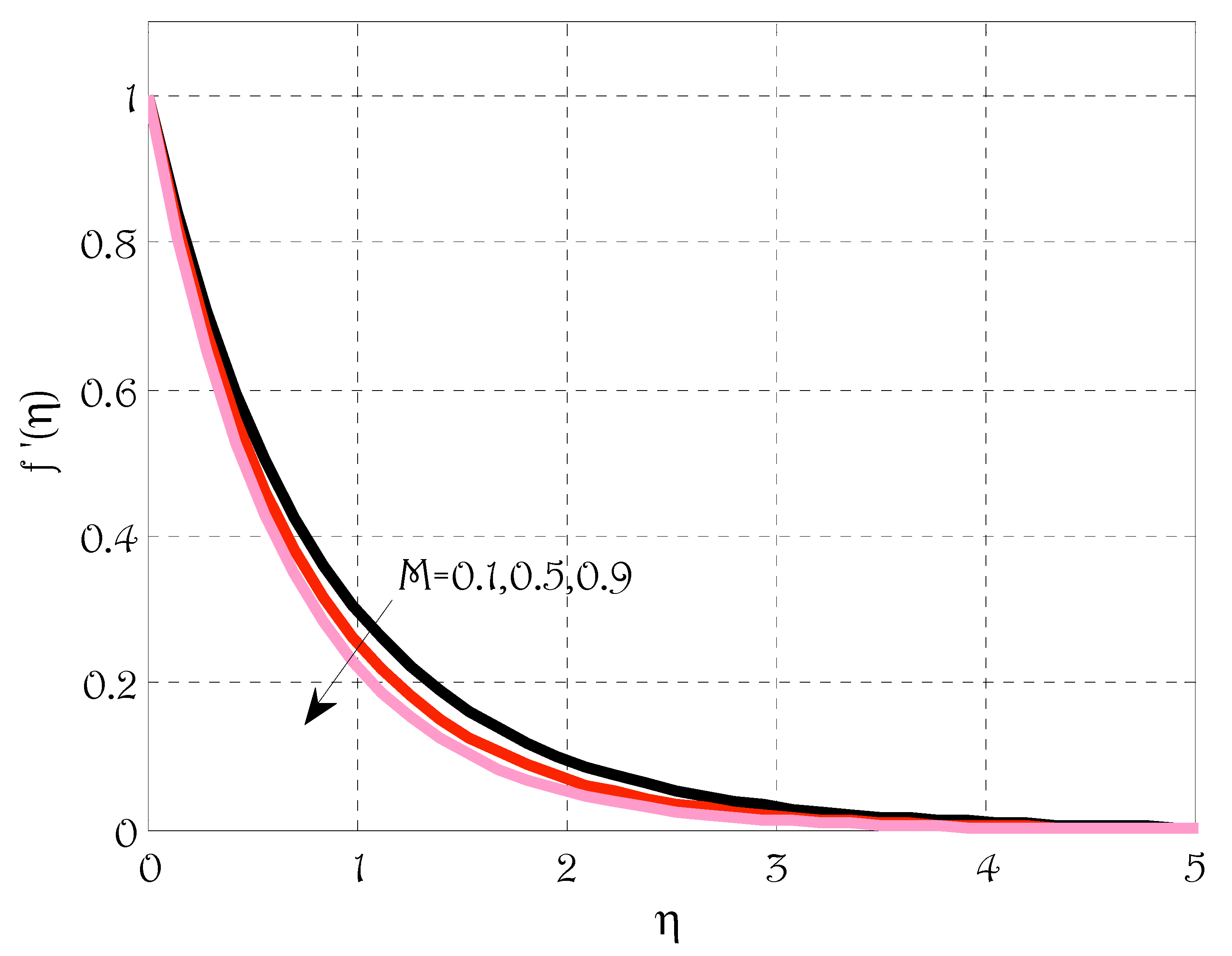
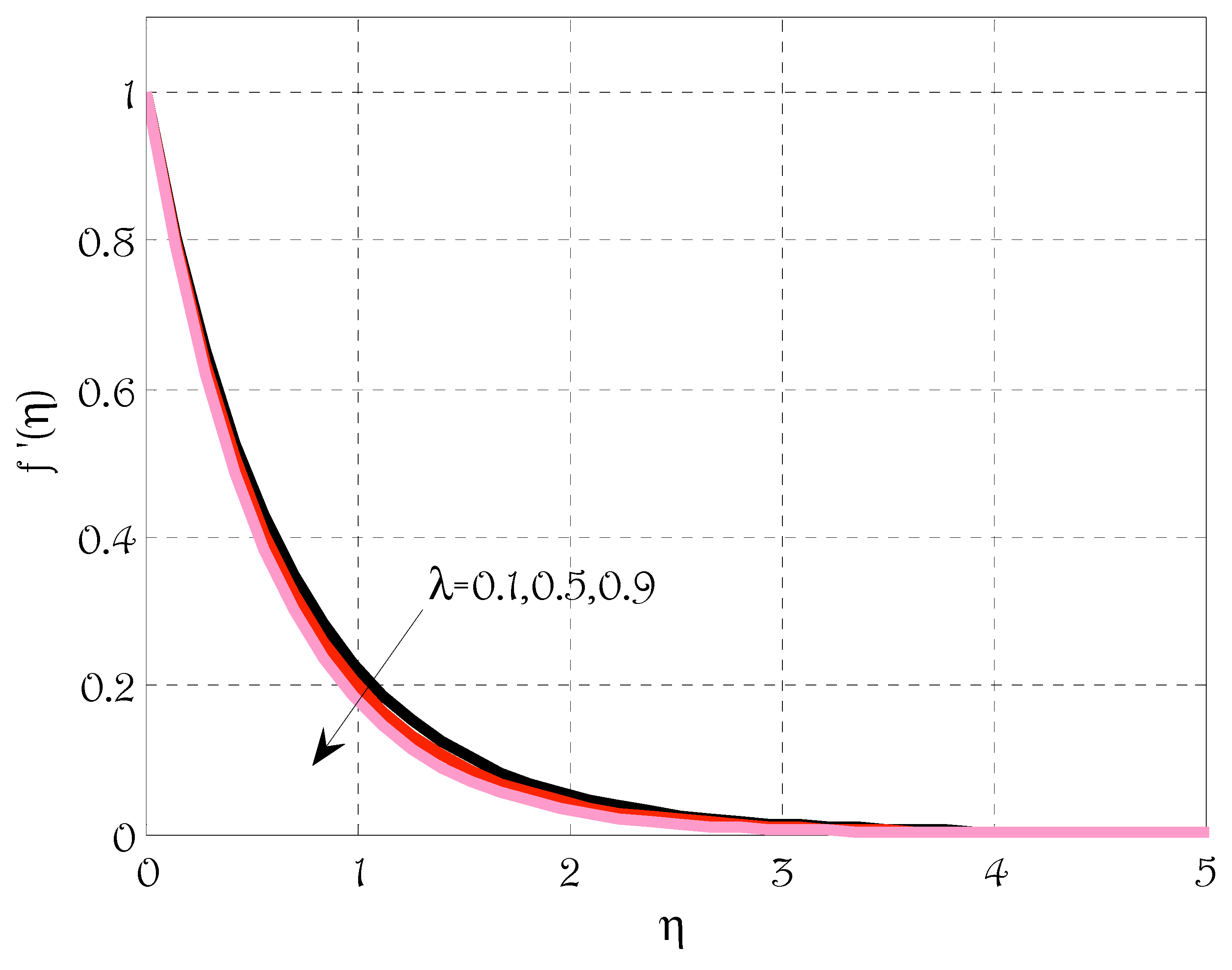
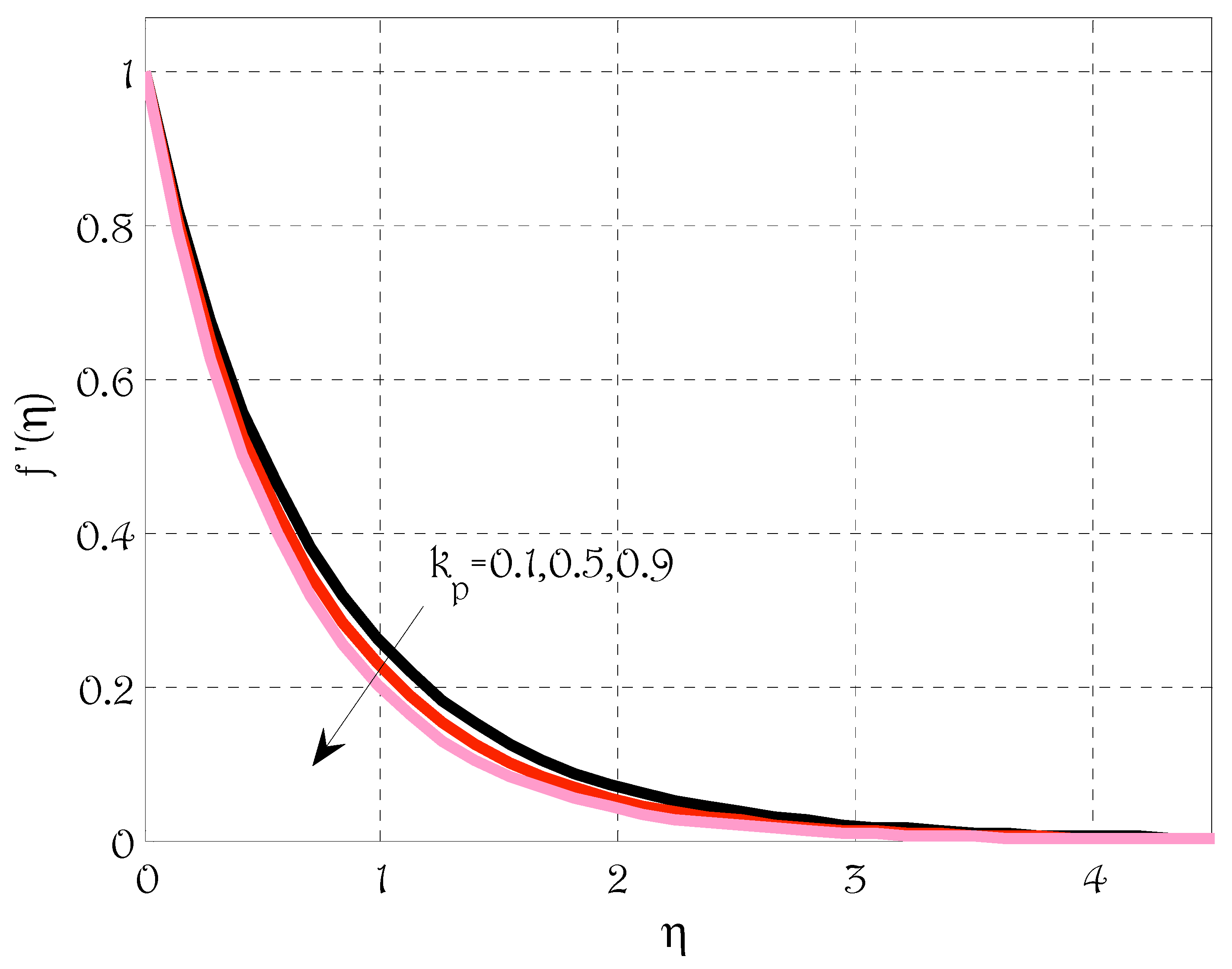
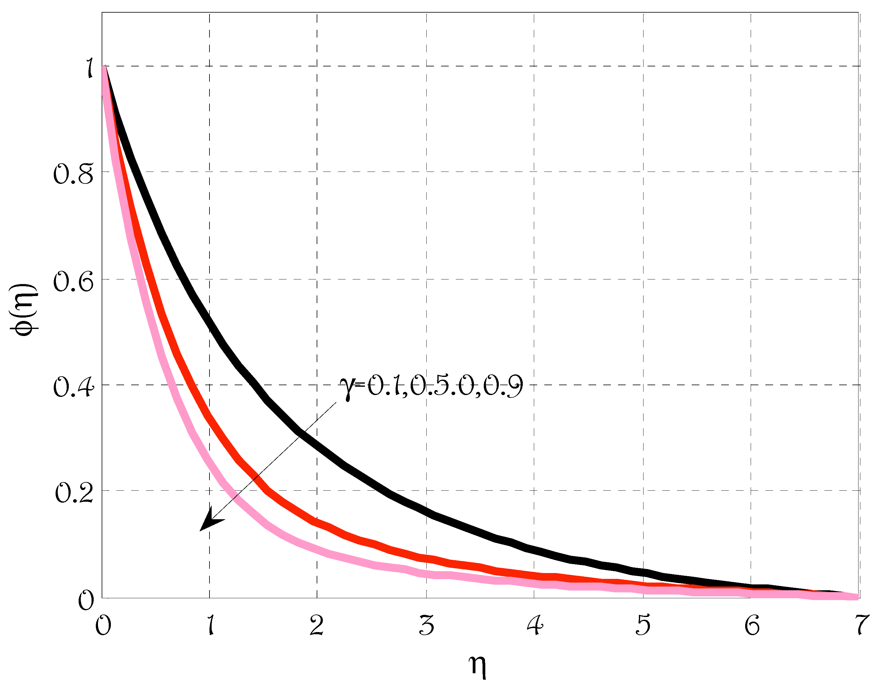
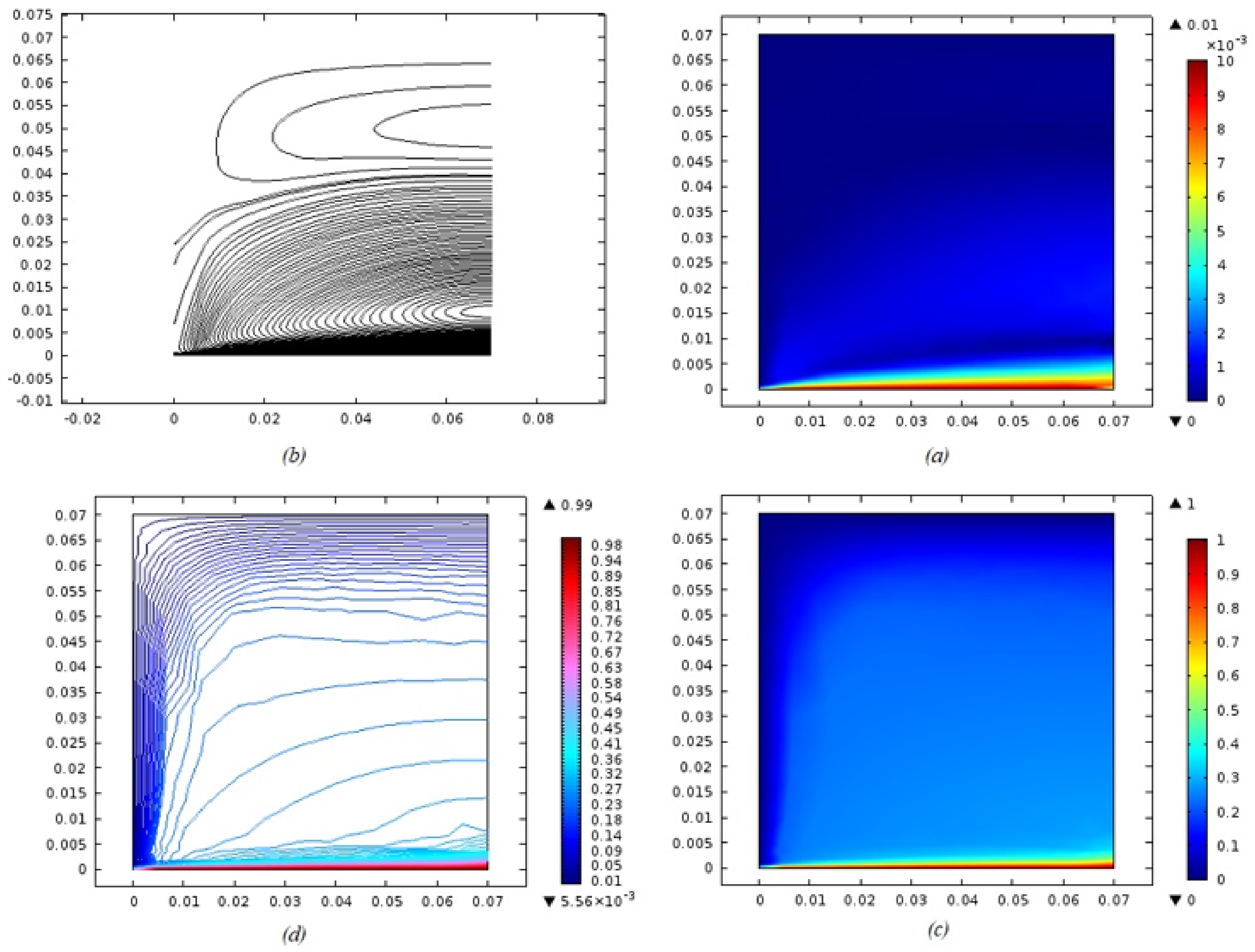
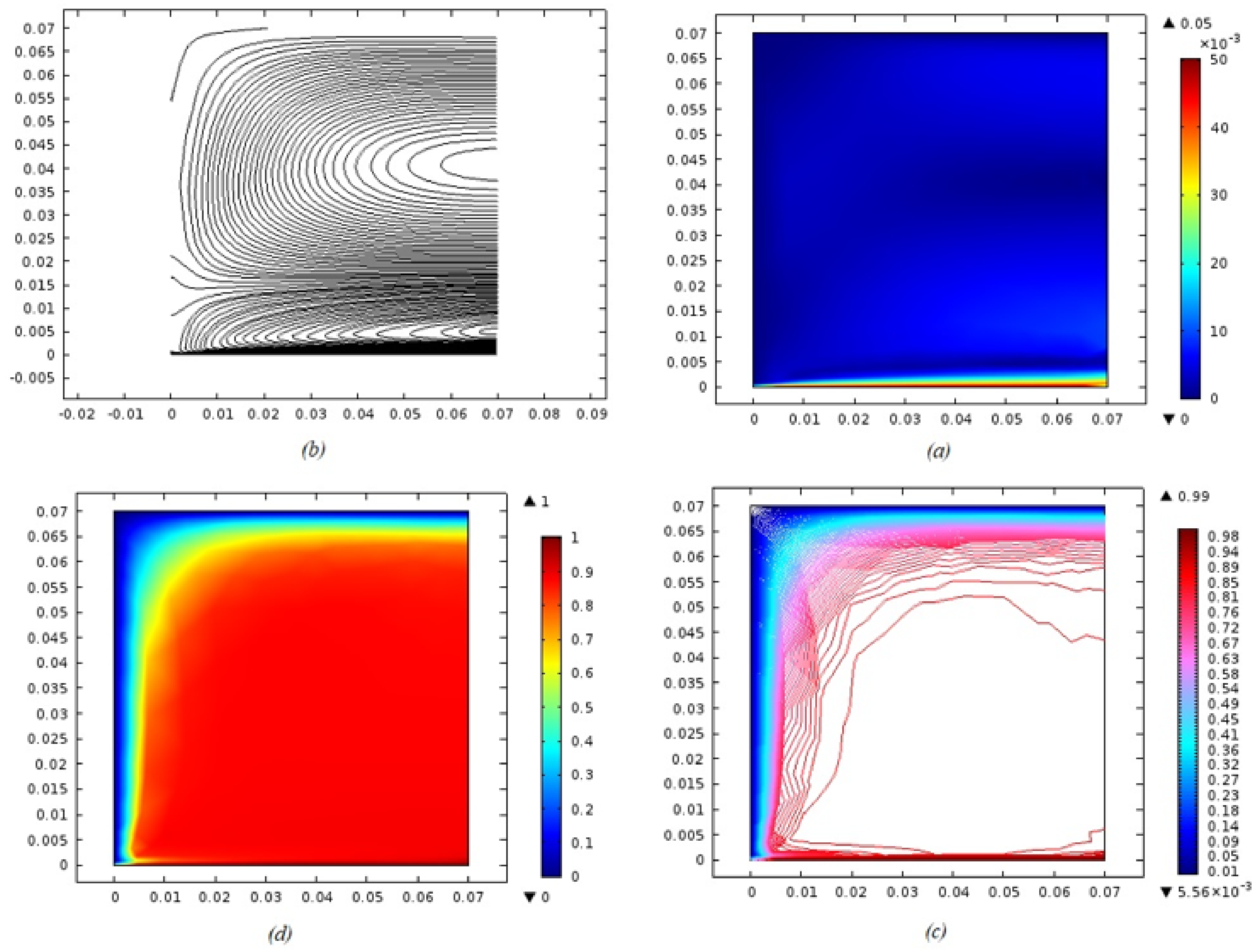
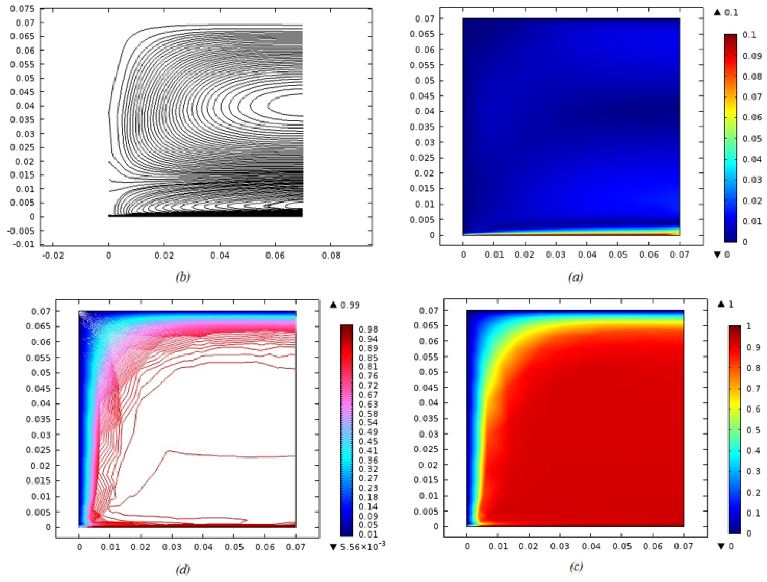
5. Results and Discussions

The finite element method employed in this study for solving ordinary differential equations is based on the Galerkin weighted residual method using weak formulations for equations with order two. The linear elements were chosen with equal lengths. Any numerical integration can be adopted for the computations of integrals due to quick calculations. The considered finite element method uses two nodes for each element. Each element produces a matrix–vector equation, and the assembly of each matrix equation corresponding to each element gives a global matrix called a stiffness matrix. By comparing the finite element method (F.E.M) with the finite difference method (F.D.M), it was concluded that F.E.M consumes less time due to utilizing fewer iterations than those utilized by F.D.M. One of the reasons behind this is the use of an iterative procedure with F.D.M. that slows the whole procedure, and the solutions’ convergence was obtained by utilizing many iterations. The F.E.M uses the linearized forms of nonlinear equations, and the computations of results are also performed by solving matrix–vector equations from the Matlab solver. The Matlab solver finds the exact solutions for matrix–vector equations, whereas the F.D.M finds the solutions of nonlinear differential equations iteratively without linearizing nonlinear equations.
Figure 1 shows the geometry of the considered problem. Figure 2, Figure 3, Figure 4, Figure 5, Figure 6, Figure 7, Figure 8, Figure 9, Figure 10, Figure 11, Figure 12 and Figure 13 are drawn by using the standard finite element method for solving differential Equations (9), (10), (26) and (27) with boundary conditions (11). Figure 2 deliberates the impact of the magnetic parameter on the velocity profile. Figure 2 shows that velocity decays by increasing magnetic parameters. This growth of velocity profile is the consequence of resistance of Lorenz force that enhances by increment in the magnetic parameter. The impact of the Deborah number λ on the velocity profile is portrayed in Figure 3. The Deborah number contains the relaxation time parameter, which states the time when the fluid obtains an equilibrium state by applying stress. Larger values of the Deborah number give larger relaxation time, which gives more resistivity of stress in the fluid or enhances the viscosity of the fluid and, consequently, a slower velocity profile is obtained. The variation in porosity parameter on velocity profile is deliberated in Figure 4. The velocity profile de-escalates by enhancing the porosity parameter because the porosity parameter enhances the resistivity in the flow, leading to decays in the velocity profile. Figure 5 shows the variation in the Prandtl number on the temperature profile. The velocity profile de-escalates by rising values of the Prandtl number. The higher Prandtl number is responsible for smaller thermal diffusivity because both have an inverse relationship. The slower thermal diffusivity reduces thermal conductivity, which yields a slower temperature profile. Figure 6 shows the impact of thermophoretic parameters on the temperature profile. The temperature profile escalates by rising values of the thermophoretic parameter. This is due to the thermophoresis phenomenon that tends to move the hot particles from the immediate vicinity of the plate to its surroundings, and consequently, the temperature rises. Figure 7 deliberates the effect of the Brownian motion parameter on the temperature profile. The temperature profile grows by enhancing the Brownian motion parameter because the escalation in the Brownian motion parameter is responsible for spreading the hotter particles due to the increase in random movement of particles, which results in a temperature rise. The effect of the Eckert number on temperature profile is portrayed in Figure 8. The temperature profile rises by enhancing the values of the Eckert number. The increment in the Eckert number gives rise to the temperature difference between wall and ambient temperature, and therefore temperature rises. The effect of the radiation parameter on the temperature profile is shown in Figure 9. The temperature rises by enhancing the radiation parameter because the energy of the flow increases by incoming radiation. The impact of the Schmidt number on the concentration profile is portrayed in Figure 10. The concentration profile gets down by boosting the values of the Schmidt number. The de-escalation in the concentration profile is the decay of mass diffusivity due to an increase in Schmidt number. Figure 11 shows the thermophoretic parameter on the concentration profile. Rising values of thermophoretic parameters boost the concentration profile. This happened due to the thermophoresis phenomenon that tends to move nanoparticles from the immediate vicinity of the plate to its surroundings, and thus concentration profile grows. Figure 12 portrays the variation in the Brownian motion parameter on the concentration profile. The concentration profile decays by enhancing the Brownian motion parameter. The boosting up of the Brownian motion parameter gives the faster random movement of nanoparticles, resulting in decays in the concentration profile. The effect of the reaction rate parameter on the concentration profile is shown in Figure 13. From this Figure 13, it can be seen that the concentration profile de-escalates by rising values of the reaction rate parameter because higher values of the reaction rate parameter create impurity in the fluid responsible for decaying the concentration profile.
Table 3 shows the numerical values of R e x 1 2 C f and R e x 1 2 N u x for Deborah number, magnetic parameter, Brownian motion parameter and thermophoretic parameter. R e x 1 2 C f grows by enhancing the Deborah number and magnetic parameter whereas R e x 1 2 N u x decays by de-escalating the Brownian motion parameter and thermophoretic parameter.
Simulations were also carried out by employing a finite element method for solving governing equations of heat transfer of Newtonian fluid under the effects of radiations over moving surface towards x -axis. The geometry consists of a four-sided rectangular shape in which two sides are used as input and output, one side is a moving boundary and the rest have a no-free boundary condition. Figure 14, Figure 15 and Figure 16 were drawn by solving partial differential equations with different velocities of the bottom surface. The momentum and thermal boundary layers can be seen in Figure 14, Figure 15 and Figure 16.

6. Conclusions

The finite element method was utilized for heat and mass transfer of non-Newtonian fluid flow over the sheet. The linear interpolation polynomials were considered in the application procedure of the finite element method. The results were also compared with those given in past research and the classical finite difference method. In addition, the simulations for heat transfer of Newtonian fluid flow model over stretching sheet were also provided by using software that implements finite element method. By using the considered iterative method, the classical finite difference method consumed more iterations, and it was computationally expensive but gave better accuracy. The concluded points can be expressed as:
  • Velocity profile was de-escalated by escalating magnetic parameter, Deborah number and porosity parameter;
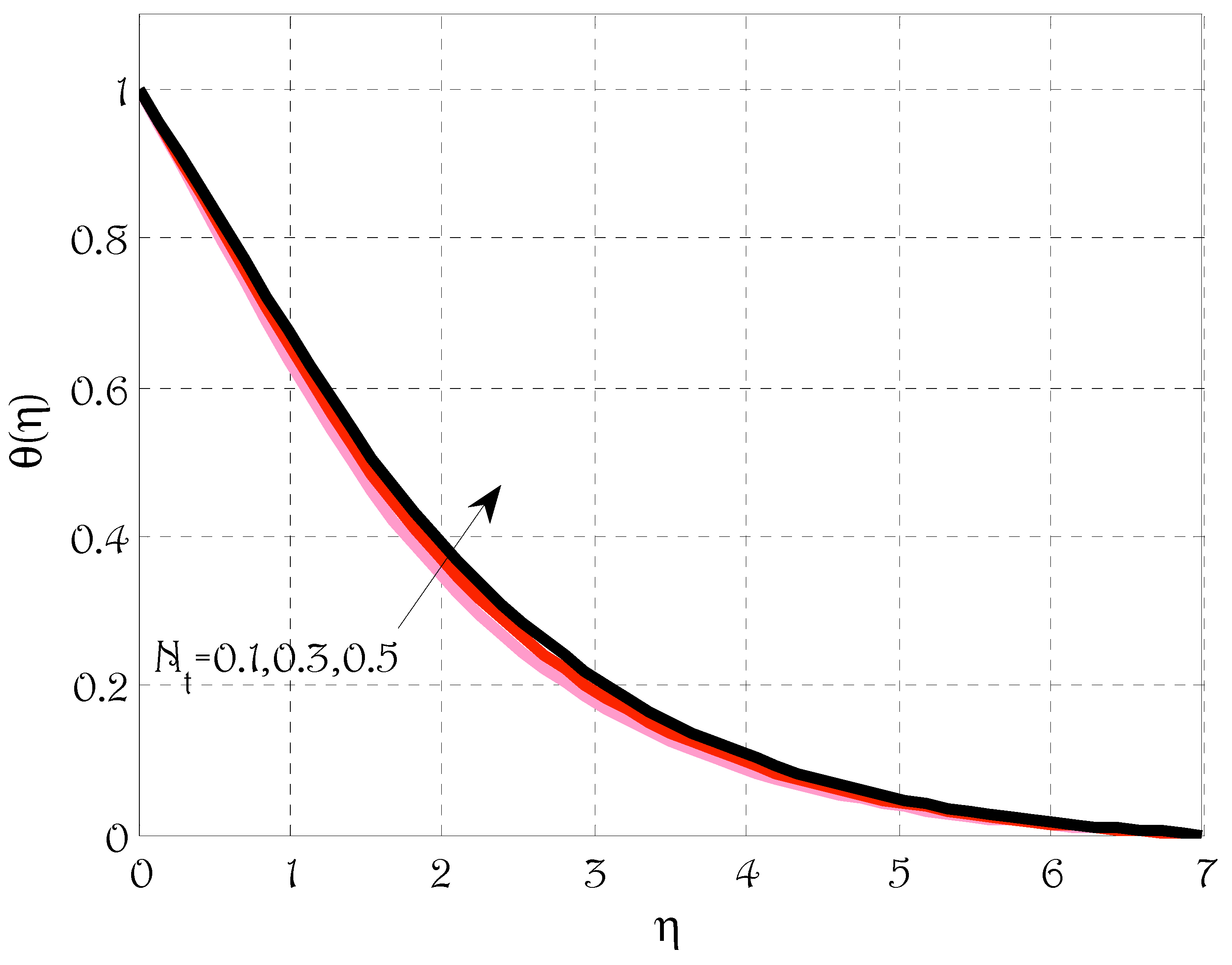
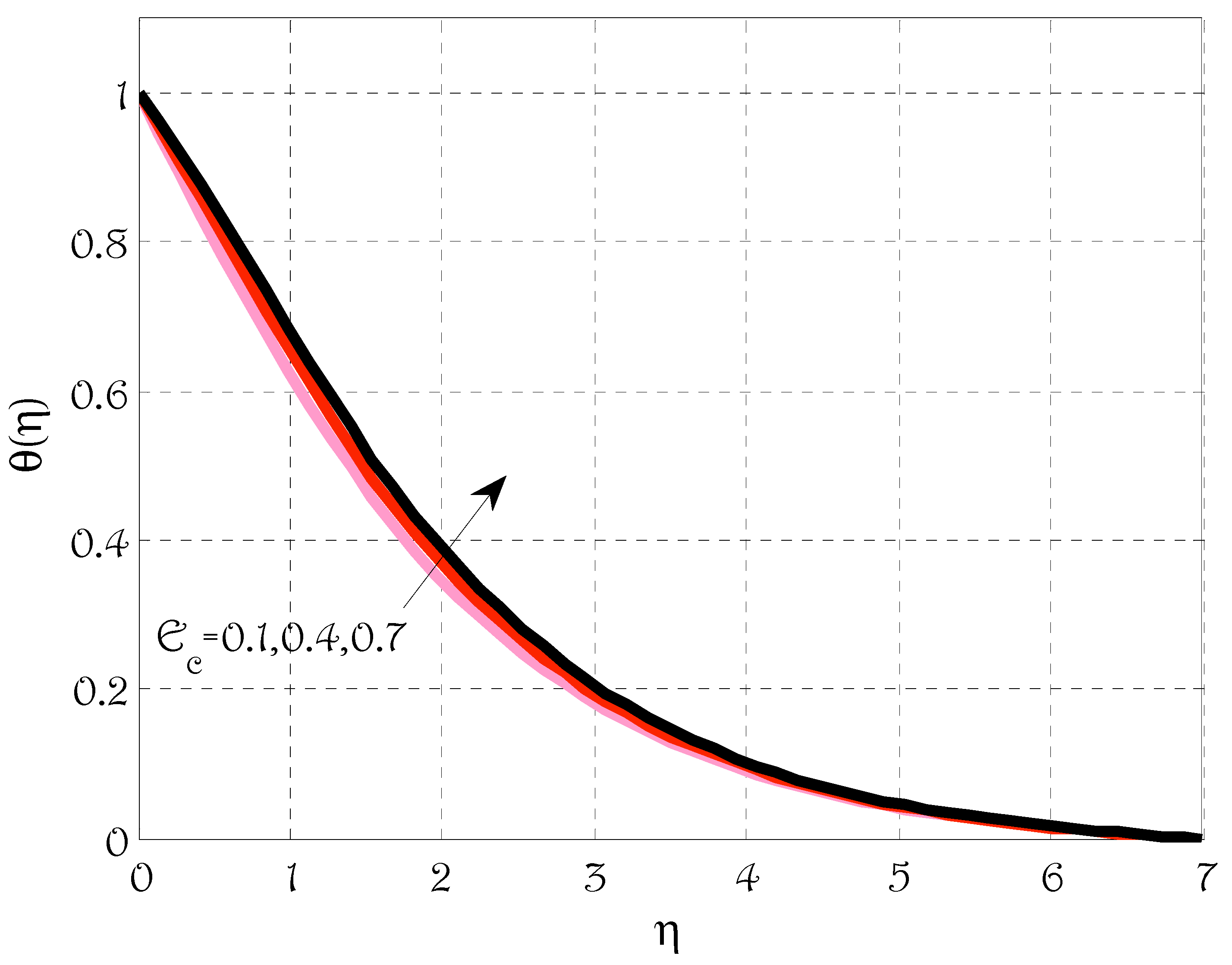
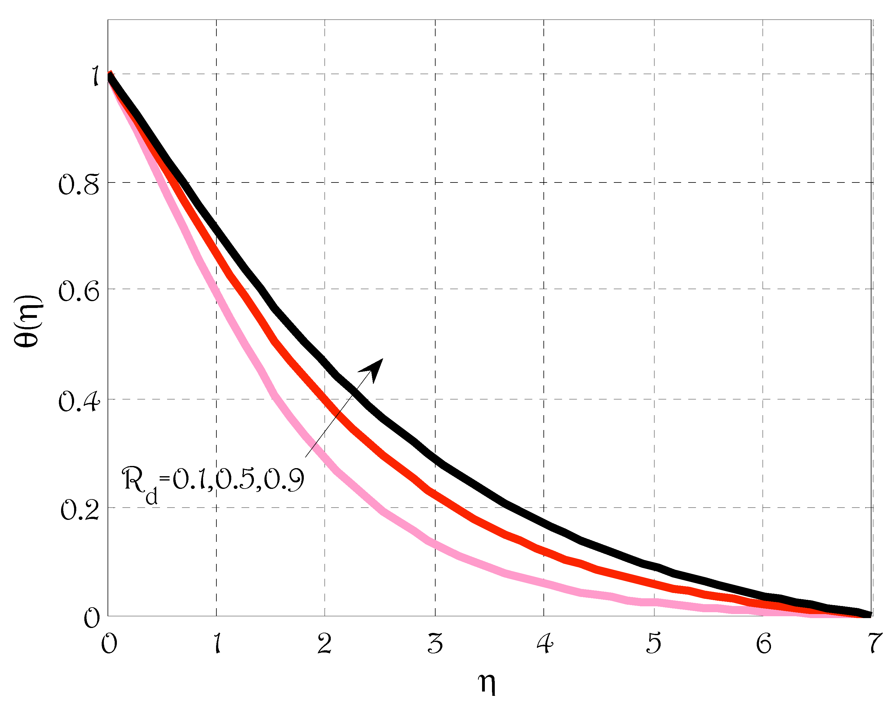
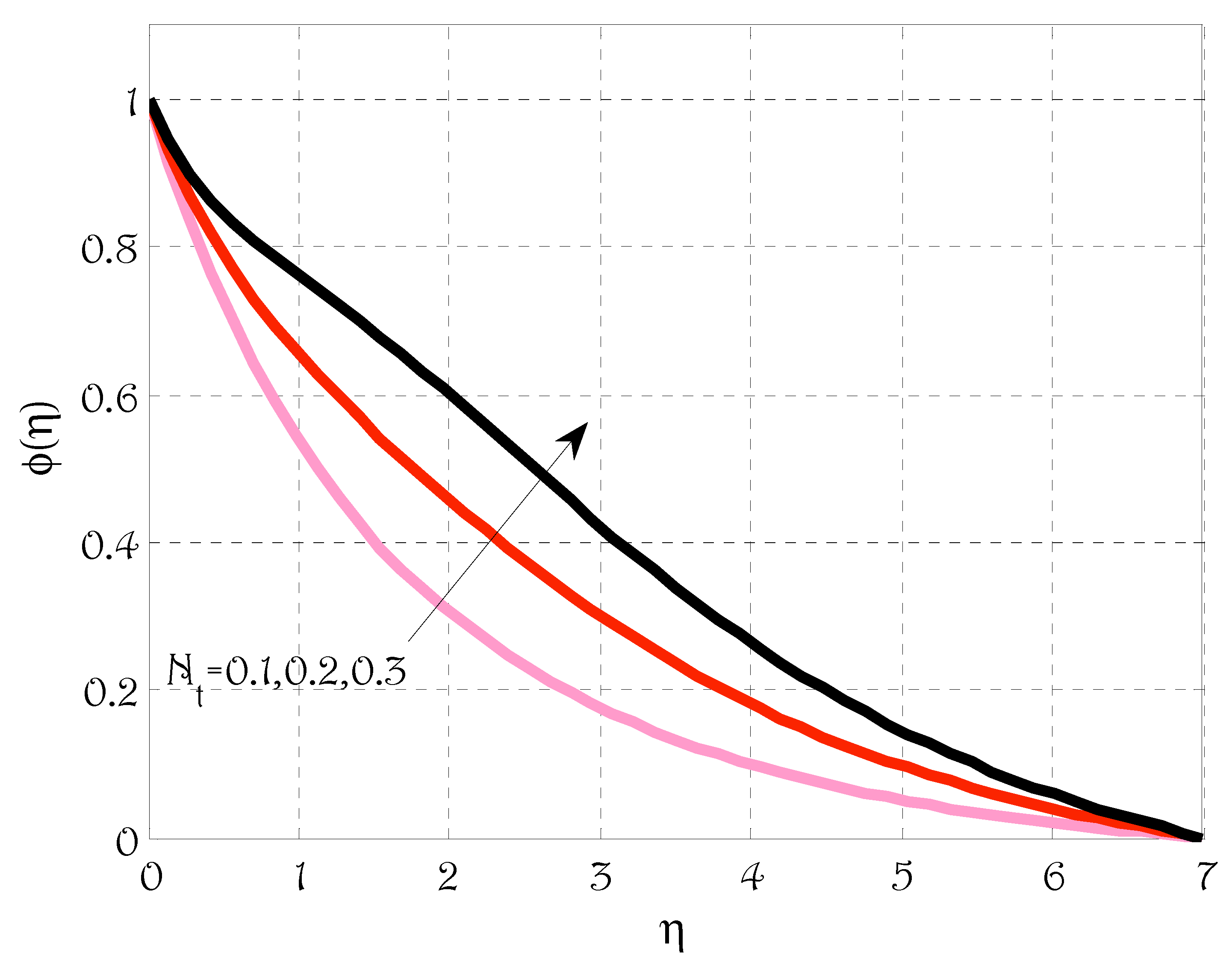
  • The temperature profile was grown by rising values of radiation parameters, Brownian motion and thermophoretic parameters;
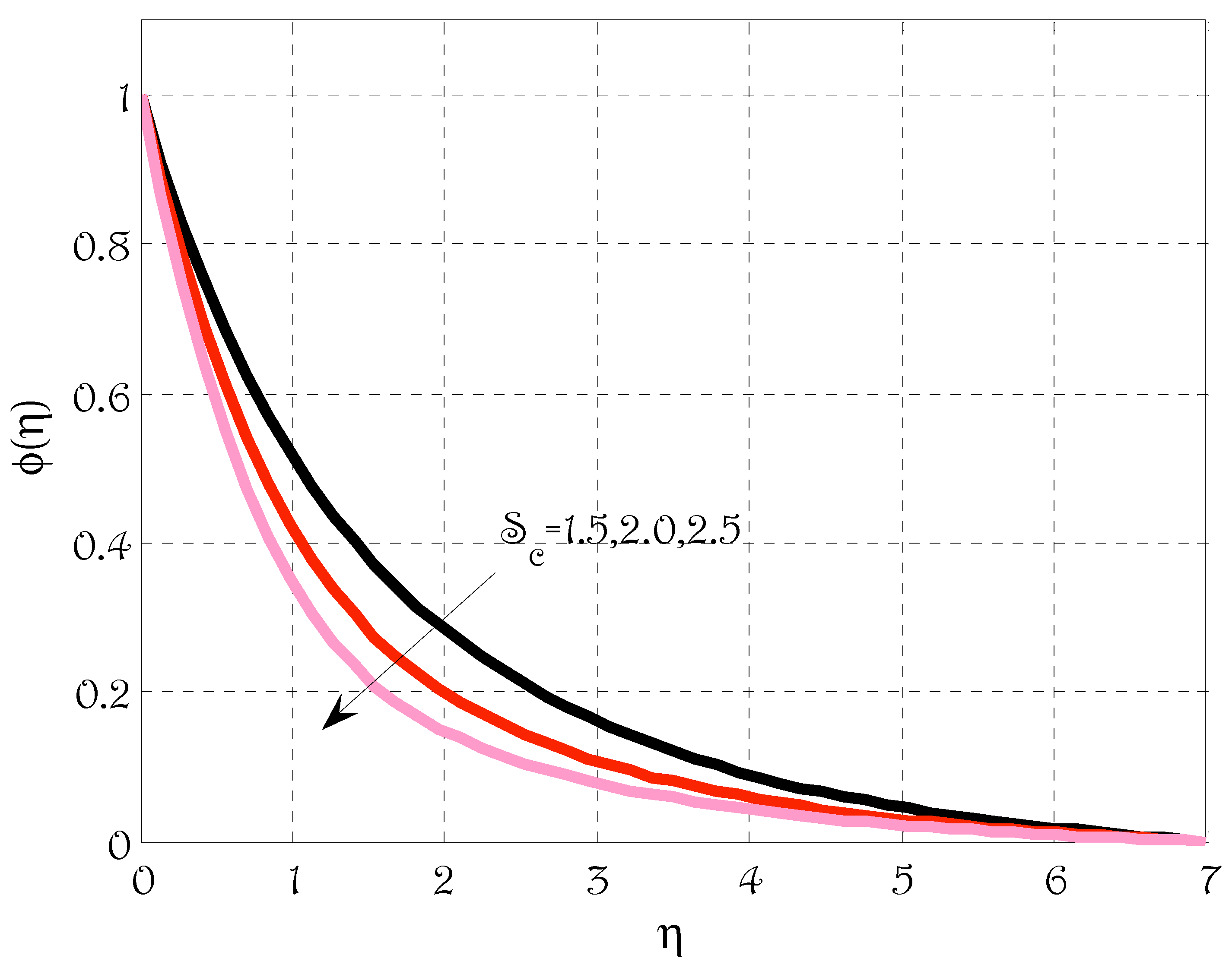
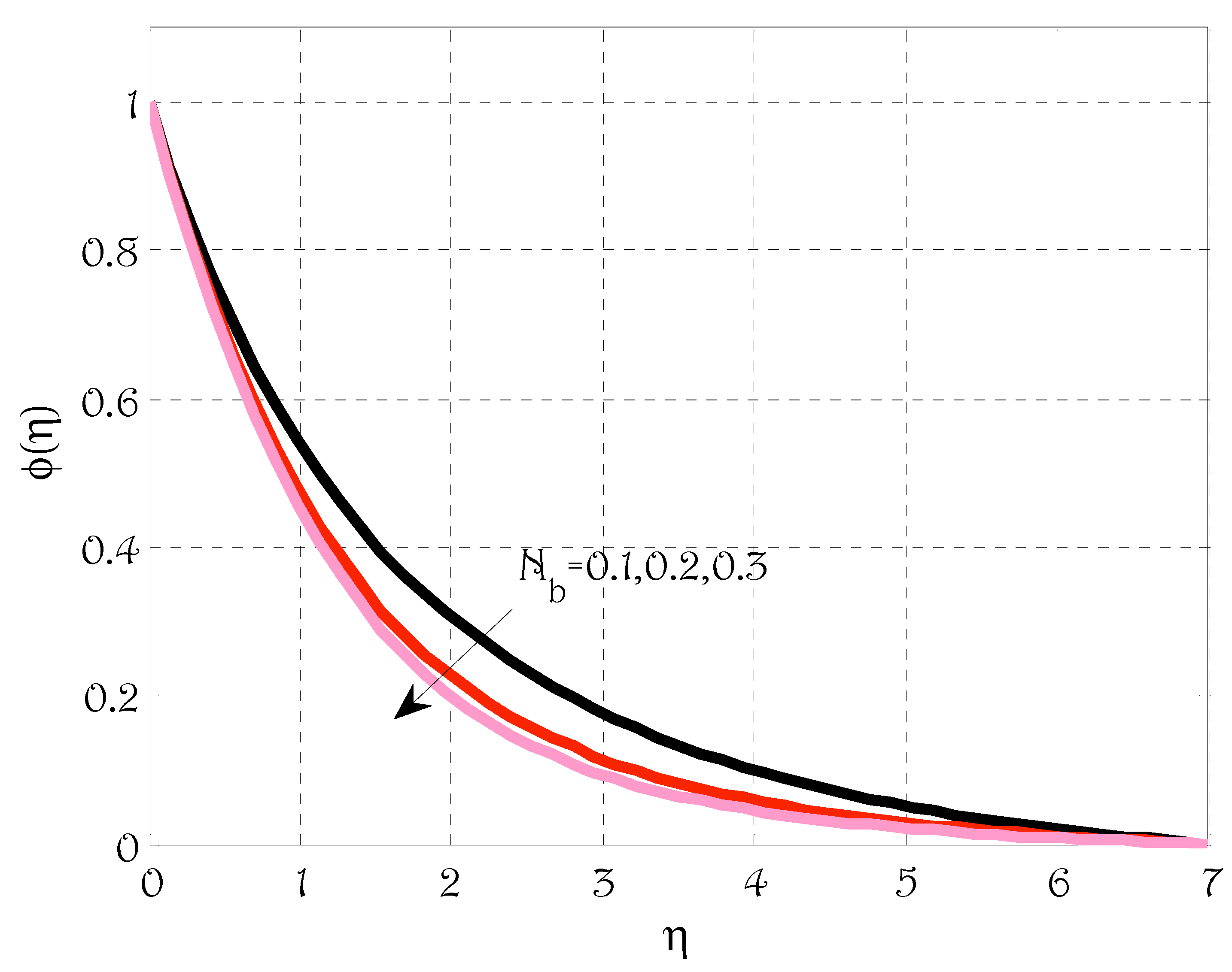
  • The concentration profile was escalated by enhancing the Brownian motion and thermophoretic parameters and de-escalating by rising Schmidt number and reaction rate parameters.
Further, the finite element method considered in this work can be employed to solve efficiently nonlinear problems of similar type that arise in computational fluid dynamics with some extra effects. Following the completion of this work, it will be possible to propose other applications for the currently employed methodology, if desired [46,47,48,49]. In addition, the developed method is easy to use and can solve a wider range of differential equations in both practice and theory.

Author Contributions

Conceptualization, methodology, and analysis, writing—review and editing, Y.N.; funding acquisition, K.A.; investigation, Y.N.; methodology, M.B.; project administration, K.A.; resources, K.A.; supervision, M.S.A.; visualization, K.A.; writing—review and editing, M.S.A.; proofreading and editing, M.B. All authors have read and agreed to the published version of the manuscript.

Funding

This work was supported by a Seed Project research grant from Prince Sultan University, Saudi Arabia (SEED-2022-CHS-100).

Data Availability Statement

The manuscript included all required data and implementing information.

Acknowledgments

The authors wish to express their gratitude to Prince Sultan University for facilitating the publication of this article through the Theoretical and Applied Sciences Lab.

Conflicts of Interest

The authors declare no conflict of interest.

References

  1. Rivlin, R.S.; Ericksen, J.L. Stress deformation relation for isotropic materials. J. Rat. Mech. Anal. 1955, 4, 323–425. [Google Scholar] [CrossRef]
  2. Hayat, T.; Awais, M. Three-dimensional flow of upperconvected Maxwell (UCM) fluid. Int. J. Numer. Methods Fluids 2011, 66, 875–884. [Google Scholar]
  3. Hayat, T.; Mustafa, M.; Shehzadand, S.A.; Obaidat, S. Melting heat transfer in the stagnation-point flow of an upper-convected Maxwell (UCM) fluid past a stretching sheet. Int. J. Numer. Methods Fluids 2012, 68, 233–243. [Google Scholar] [CrossRef]
  4. Mukhopadhyay, S. Upper-Convected Maxwell Fluid Flow over an Unsteady Stretching Surface Embedded in Porous Medium Subjected to Suction/Blowing. Z. Nat. A 2012, 67, 641–646. [Google Scholar] [CrossRef] [Green Version]
  5. Adegbie, K.S.; Omowaye, A.J.; Disu, A.B.; Animasaun, I.L. Heat and Mass Transfer of Upper Convected Maxwell Fluid Flow with Variable Thermo-Physical Properties over a Horizontal Melting Surface. Appl. Math. 2015, 6, 1362–1379. [Google Scholar] [CrossRef] [Green Version]
  6. Maxwell, J.C. On the dynamical theory of gases. In The Kinetic Theory of Gases: An Anthology of Classic Papers with Historical Commentary, Philosophical Transactions of the Royal Society of London; Cambridge University Press: Cambridge, UK, 2003; pp. 197–261. [Google Scholar]
  7. Mukhopadhyay, S.; Bhattacharyya, K. Unsteady flow of a Maxwell fluid over a stretching surface in presence of chemical reaction. J. Egypt. Math. Soc. 2012, 20, 229–234. [Google Scholar] [CrossRef] [Green Version]
  8. Nadeem, S.; Ahmad, S.; Muhammad, N. Cattaneo-Christov flux in the flow of a viscoelastic fluid in the presence of Newtonian heating. J. Mol. Liquids 2017, 237, 180–184. [Google Scholar] [CrossRef]
  9. Nadeem, S.; Ahmad, S.; Muhammad, N.; Mustafa, M. Chemically reactive species in the flow of a Maxwell fluid. Results Phys. 2017, 7, 2607–2613. [Google Scholar] [CrossRef]
  10. Khan, M.; Malik, M.Y.; Salahuddin, T.; Khan, F. Generalized diffusion effects on Maxwell nanofluid stagnation point flow over a stretchable sheet with slip conditions and chemical reaction. J. Braz. Soc. Mech. Sci. Eng. 2019, 41, 138. [Google Scholar] [CrossRef] [Green Version]
  11. Yang, W.; Chen, X.; Zhang, X.; Zheng, L.; Liu, F. Flow and heat transfer of double fractional Maxwell fluids over a stretching sheet with variable thickness. Appl. Math. Model. 2020, 80, 204–216. [Google Scholar]
  12. Wang, F.; Liu, J. The first solution for the helical flow of a generalized Maxwell fluid within annulus of cylinders by new definition of transcendental function. Math. Probl. Eng. 2020, 2020, 8919817. [Google Scholar] [CrossRef]
  13. Recebli, Z.; Selimli, S.; Gedik, E. Three dimensional numerical analysis of magnetic field effect on Convective heat transfer during the MHD steady state laminar flow of liquid lithium in a cylindrical pipe. Comput. Fluids 2013, 15, 410–417. [Google Scholar] [CrossRef]
  14. Recebli, Z.; Selimli, S.; Ozkaymak, M. Theoretical analyses of immiscible MHD pipe flow. Int. J. Hydrogen Energy 2015, 40, 15365–15373. [Google Scholar] [CrossRef]
  15. Selimli, S.; Recebli, Z.; Arcaklioglu, E. Combined effects of magnetic and electrical field on the hydrodynamic and thermophysical parameters of magnetoviscous fluid flow. Int. J. Heat Mass Transf. 2015, 86, 426–432. [Google Scholar] [CrossRef]
  16. Hayat, T.; Waqas, M.; Ijaz Khan, M.; Alsaedi, A. Impacts of constructive and destructive chemical reactions in magnetohydrodynamic (MHD) flow of Jeffrey liquid due to nonlinear radially stretched surface. J. Mol. Liq. 2017, 225, 302–310. [Google Scholar] [CrossRef]
  17. Hayat, T.; Abbas, Z.; Sajid, M. Series solution for the upperconvected Maxwell fluid over a porous stretching plate. Phys. Lett. A 2006, 358, 396–403. [Google Scholar] [CrossRef]
  18. Raftari, B.; Yildirim, A. The application of homotopy perturbation method for MHD flows of UCM fluids above porous stretching sheets. Comput. Math. Appl. 2010, 59, 3328–3337. [Google Scholar] [CrossRef] [Green Version]
  19. Sajid, M.; Iqbal, Z.; Hayat, T.; Obaidat, S. Series Solution for Rotating Flow of an Upper Convected Maxwell Fluid over a Stretching Sheet. Commun. Theor. Phys. 2011, 56, 740–744. [Google Scholar] [CrossRef]
  20. Abel, M.S.; Tawade, J.V.; Nandeppanavar, M.M. MHD flow and heat transfer for the upper-convected Maxwell fluid over a stretching sheet. Meccanica 2012, 47, 385–393. [Google Scholar]
  21. Abbasi, M.; Rahimipetroudi, I. Analytical solution of an upperconvective Maxwell fluid in porous channel with slip at the boundaries by using the Homotopy Perturbation Method. IJNDES 2013, 5, 7–17. [Google Scholar]
  22. Nadeem, S.; Ul Haq, R.; Khan, Z.H. Numerical study of MHD boundary layer flow of a Maxwell fluid past a stretching sheet in the presence of nanoparticles. J. Taiwan Inst. Chem. E. 2014, 45, 121–126. [Google Scholar] [CrossRef]
  23. Afify, A.A.; Elgazery, N.S. Effect of a chemical reaction on magnetohydrodynamic boundary layer flow of a Maxwell fluid over a stretching sheet with nanoparticles. Particuology 2016, 29, 154–161. [Google Scholar] [CrossRef]
  24. Sarpkaya, T. Flow of non-Newtonian fluids in a magnetic field. AIChE J. 1961, 7, 324–328. [Google Scholar] [CrossRef]
  25. Turkyilmazoglu, M. Thermal radiation effects on the time-dependent MHD permeable flow having a variable viscosity. Int. J. Therm. Sci. 2011, 50, 88–96. [Google Scholar] [CrossRef]
  26. Turkyilmazoglu, M. Multiple analytic solutions of heat and mass transfer of magnetohydrodynamic slip flow for two types of viscoelastic fluids over a stretching surface. J. Heat Transfer. 2012, 134, 071701. [Google Scholar] [CrossRef]
  27. Dhanai, R.; Rana, P.; Kumar, L. Multiple solutions in MHD flow and heat transfer of Sisko fluid containing nanoparticles migration with a convective boundary condition: Critical points. Eur. Phys. J. Plus 2016, 131, 142. [Google Scholar] [CrossRef]
  28. Ellahi, R.; Bhatti, M.M.; Pop, I. Effects of hall and ion slip on MHD peristaltic flow of Jeffrey fluid in a nonuniform rectangular duct. Int. J. Numer. Methods Heat Fluid Flow 2016, 26, 1802–1820. [Google Scholar] [CrossRef]
  29. Ahmad, S.; Nadeem, S. Flow analysis by Cattaneo–Christov heat flux in the presence of Thomson and Troian slip condition. Appl. Nanosci. 2020, 10, 4673–4687. [Google Scholar] [CrossRef]
  30. Farooq, U.; Lu, D.; Munir, S.; Ramzan, M.; Suleman, M.; Hussain, S. MHD flow of Maxwell fluid with nanomaterials due to an exponentially stretching surface. Sci. Rep. 2019, 9, 7312. [Google Scholar] [CrossRef] [Green Version]
  31. Ramadevi, B.; Sugunamma, V.; Kumar, A.; Ramana, R.J.V. MHD flow of Carreau fluid over a variable thickness melting surface subject to Cattaneo-Christov heat flux. Multidiscip. Modeling Mater. Struct. 2019, 15, 2–25. [Google Scholar]
  32. Kumar, K.A.; Reddy, J.V.R.; Sugunamma, V.; Sandeep, N. MHD Carreau fluid flow past a melting surface with Cattaneo-Christov heat flux. In Applied Mathematics and Scientific Computing; Rushi Kumar, B., Sivaraj, R., Prasad, B., Nalliah, M., Reddy, A., Eds.; Birkhäuser: Cham, Switzerland, 2019; pp. 325–336. [Google Scholar]
  33. Fourier, J.B.J. Theorie analytique de la chaleur, paris. Acad. Sci. 1822, 3, 1–636. [Google Scholar]
  34. Fick, A. Poggendorff’s flannel. Ann. Phys. Chem. 1855, 170, 59–86. [Google Scholar] [CrossRef]
  35. Javed, F.; Nadeem, S. Numerical solution of a Casson nanofluid flow and heat transfer analysis between concentric cylinders. J. Power Technol. 2019, 99, 25–30. [Google Scholar]
  36. Mallawi, F.; Bhuvaneswari, M.; Sivasankaran, S.; Eswaramoorthi, S. Impact of double-stratification on convective flow of a non-Newtonian liquid in a Riga plate with CattaneoChristov double-flux and thermal radiation. Ain Shams Eng. J. 2020, 12, 969–981. [Google Scholar] [CrossRef]
  37. Sheikholeslami, M.; Farshad, S.A.; Shafee, A.; Babazadeh, H. Performance of solar collector with turbulator involving nanomaterial turbulent regime. Renew. Energy 2021, 163, 1222–1237. [Google Scholar] [CrossRef]
  38. Sheikholeslami, M.; Farshad, S.A. Nanoparticle transportation inside a tube with quad-channel tapes involving solar radiation. Powder Technol. 2021, 378, 145–159. [Google Scholar] [CrossRef]
  39. Waqas, H.; Farooq, U.; Alshehri, H.M.; Goodarzi, M. Marangoni-bioconvectional flow of Reiner–Philippoff nanofluid with melting phenomenon and nonuniform heat source/sink in the presence of a swimming microorganisms. Math. Methods Appl. Sci. 2021, 1–19. [Google Scholar] [CrossRef]
  40. Alazwari, M.A.; Abu-Hamdeh, N.H.; Goodarzi, M. Entropy Optimization of First-Grade Viscoelastic Nanofluid Flow over a Stretching Sheet by Using Classical Keller-Box Scheme. Mathematics 2021, 9, 2563. [Google Scholar] [CrossRef]
  41. Alazwari, M.; Safaei, M. Non-isothermal hydrodynamic characteristics of a nanofluid in a fin-attached rotating tube bundle. Mathematics 2021, 9, 1153. [Google Scholar] [CrossRef]
  42. Fetecau, C.; Ellahi, R.; Sait, S.M. Mathematical Analysis of Maxwell Fluid Flow through a Porous Plate Channel Induced by a Constantly Accelerating or Oscillating Wall. Mathematics 2021, 9, 90. [Google Scholar] [CrossRef]
  43. Nawaz, Y.; Arif, M.S. An effective modification of finite element method for heat and mass transfer of chemically reactive unsteady flow. Comput. Geosci. 2020, 24, 275–291. [Google Scholar] [CrossRef]
  44. Sadiq, M.A.; Hayat, T. Darcy–Forchheimer flow of magneto Maxwell liquid bounded by convectively heated sheet. Results Phys. 2016, 6, 884–890. [Google Scholar] [CrossRef] [Green Version]
  45. Turkyilmazoglu, M. The analytical solution of mixedconvection heat transfer and fluid flow of a MHD viscoelastic fluid over a permeable stretching surface. Int. J. Mech. Sci. 2013, 77, 263–268. [Google Scholar] [CrossRef]
  46. Nawaz, Y.; Arif, M.S.; Shatanawi, W.; Nazeer, A. An explicit fourth-order compact numerical scheme for heat transfer of boundary layer flow. Energies 2021, 14, 3396. [Google Scholar] [CrossRef]
  47. Nawaz, Y.; Arif, M.S.; Shatanawi, W.; Ashraf, M.U. A Fourth Order Numerical Scheme for Unsteady Mixed Convection Boundary Layer Flow: A Comparative Computational Study. Energies 2022, 15, 910. [Google Scholar] [CrossRef]
  48. Nawaz, Y.; Arif, M.S.; Shatanawi, W. A New Fourth-Order Predictor–Corrector Numerical Scheme for Heat Transfer by Darcy–Forchheimer Flow of Micropolar Fluid with Homogeneous–Heterogeneous Reactions. Appl. Sci. 2022, 12, 6072. [Google Scholar] [CrossRef]
  49. Nawaz, Y.; Arif, M.S.; Abodayeh, K. A Compact Numerical Scheme for the Heat Transfer of Mixed Convection Flow in Quantum Calculus. Appl. Sci. 2022, 12, 4959. [Google Scholar] [CrossRef]
Figure 1. Geometry of the problem.
Energies 15 04713 g001
Figure 2. Effect of magnetic parameter M on velocity profile f using λ = 0.1 ,   k p = 0.1 ,   R d = 0.7 ,   P r = 1.9 ,   E c = 0.1 ,   N b = 0.1 ,   N t = 0.1 ,   S c = 1.4 ,   γ = 0.1 .
Energies 15 04713 g002
Figure 3. Effect of Deborah number λ on velocity profile f using M = 0.5 ,   k p = 0.5 ,   R d = 0.7 ,   P r = 1.9 ,   E c = 0.1 ,   N b = 0.1 ,   N t = 0.1 ,   S c = 1.4 ,   γ = 0.1 .
Energies 15 04713 g003
Figure 4. Effect of porosity parameter k p on velocity profile f using λ = 0.1 ,   M = 0.5 ,   R d = 0.7 ,   P r = 1.9 ,   E c = 0.1 ,   N b = 0.1 ,   N t = 0.1 ,   S c = 1.4 ,   γ = 0.1 .
Energies 15 04713 g004
Figure 5. Effect of Prandtl number P r on temperature profile θ using k p = 0.5 ,   M = 0.5 ,   R d = 0.7 ,   λ = 0.1 ,   E c = 0.1 ,   N b = 0.1 ,   N t = 0.3 ,   S c = 1.4 ,   γ = 0.1 .
Energies 15 04713 g005
Figure 6. Effect of thermophoretic parameter N t on temperature profile θ using k p = 0.5 ,   M = 0.5 ,   R d = 0.7 ,   λ = 0.1 ,   E c = 0.1 ,   N b = 0.1 ,   P r = 1.9 ,   S c = 1.4 ,   γ = 0.1 .
Energies 15 04713 g006
Figure 7. Effect of Brownian motion parameter N b on temperature profile θ using k p = 0.5 ,   M = 0.5 ,   R d = 0.7 ,   λ = 0.1 ,   E c = 0.1 ,   N t = 0.1 ,   P r = 1.9 ,   S c = 1.4 ,   γ = 0.1 .
Energies 15 04713 g007
Figure 8. Effect of Eckert number E c on temperature profile θ using k p = 0.5 ,   M = 0.5 ,   R d = 0.7 ,   λ = 0.1 ,   N t = 0.3 ,   N b = 0.1 ,   P r = 1.9 ,   S c = 1.4 ,   γ = 0.1 .
Energies 15 04713 g008
Figure 9. Effect of radiation parameter R d on temperature profile θ using k p = 0.5 ,   M = 0.5 ,   E c = 0.4 ,   λ = 0.7 ,   N t = 0.1 ,   N b = 0.1 ,   P r = 1.5 ,   S c = 1.5 ,   γ = 0.1 .
Energies 15 04713 g009
Figure 10. Effect of Schmidt number S c on concentration profile ϕ using k p = 0.5 ,   M = 0.5 ,   E c = 0.4 ,   λ = 0.1 ,   N t = 0.1 ,   N b = 0.1 ,   P r = 1.5 ,   R d = 0.7 ,   γ = 0.1 .
Energies 15 04713 g010
Figure 11. Effect of thermophoretic parameter N t on concentration profile ϕ using k p = 0.5 ,   M = 0.5 ,   E c = 0.4 ,   λ = 0.1 ,   S c = 1.4 ,   N b = 0.1 ,   P r = 1.5 ,   R d = 0.7 ,   γ = 0.1 .
Energies 15 04713 g011
Figure 12. Effect of Brownian motion parameter N b on concentration profile ϕ using k p = 0.5 ,   M = 0.5 ,   E c = 0.4 ,   λ = 0.1 ,   S c = 1.4 ,   N t = 0.1 ,   P r = 1.5 ,   R d = 0.7 ,   γ = 0.1 .
Energies 15 04713 g012
Figure 13. Effect of reaction rate parameter γ on concentration profile ϕ using k p = 0.5 ,   M = 0.5 ,   E c = 0.4 ,   λ = 0.1 ,   S c = 1.5 ,   N t = 0.1 ,   P r = 1.5 ,   R d = 0.7 ,   N b = 0.1 .
Energies 15 04713 g013
Figure 14. (a) Surface plot for velocity; (b) streamlines; (c) surface plot for temperature; (d) isothermal contours using M = 0.5 ,   k p = 1 ,   U w = 0.01 .
Energies 15 04713 g014
Figure 15. (a) Surface plot for velocity; (b) streamlines; (c) surface plot for temperature; (d) isothermal contours using M = 0.5 ,   k p = 1 ,   U w = 0.05 .
Energies 15 04713 g015
Figure 16. (a) Surface plot for velocity; (b) streamlines; (c) surface plot for temperature; (d) isothermal contours using M = 0.5 ,   k p = 1 ,   U w = 0.1 .
Energies 15 04713 g016
Table 1. Meshfree analysis for f ,   θ and ϕ with varying amounts of elements using = 0.9 ,   P r = 1.5 ,   S c = 1.5 ,   E c = 0.4 ,   N b = 0.1 ,   N t = 0.1 ,   R d = 0.3 ,   k p = 0.7 ,   λ = 0.7 ,   γ = 0.1 .
N o .   o f   E l e m e n t s / N o d e s f ( 0.84 ) θ ( 0.84 ) ϕ ( 0.84 )
F.E.Mbvp4cF.E.Mbvp4cF.E.Mbvp4c
50 0.2134 0.4341 0.7078 0.7355 0.6168 0.6034
100 0.4630 0.2942 0.8587 0.8934 0.7769 0.7509
150 0.5991 0.2190 0.9085 0.9403 0.8432 0.8172
200 0.6814 0.1738 0.9327 0.9606 0.8793 0.8556
250 0.7360 0.1439 0.9468 0.9715 0.9019 0.8807
300 0.7747 0.1227 0.9561 0.9780 0.9174 0.8984
350 0.8036 0.1069 0.9626 0.9823 0.9287 0.9115
400 0.8260 0.0948 0.9675 0.9853 0.9373 0.9216
450 0.8438 0.0851 0.9712 0.9875 0.9440 0.9297
500 0.8583 0.0771 0.9742 0.9891 0.9495 0.9362
600 0.8805 0.0650 0.9786 0.9915 0.9577 0.9462
Table 2. Comparison of presents approaches with past research for computing numerical values of f 0 using λ = 0 = M .
k p f 0
Ref. [45]Ref. [44]Present
F.E.MM.F.E.MF.D.M
0.0 1.00000 1.00000 1.05175 1.13734 0.99419
0.5 1.22474487 1.01980 1.22244 1.33431 1.21340
1.0 1.41421356 1.11803 1.36634 1.50366 1.39664
Table 3. Numerical values and comparisons of finite element methods and finite difference methods using P r = 1.5 , = S c ,   E c = 0.4 ,   R d = 0.7 ,   k p = 0.5 ,   γ = 0.9 .
λ M N b N t R e x 1 2 C f R e x 1 2 N u x
F.E.MM.F.E.MF.D.MF.E.MM.F.E.MF.D.M
0.1 0.4 0.1 0.1 2.7109 2.9783 2.7641 0.5934 0.5765 0.3927
0.7 2.9009 3.1864 2.9978 0.5587 0.5416 0.3039
0.5 0.1 2.6790 2.9272 2.7176 0.5909 0.5742 0.3849
0.9 3.0802 3.4098 3.2292 0.5400 0.5228 0.2557
0.4 0.1 2.8385 3.1178 2.9210 0.5695 0.5525 0.3322
0.2 2.8385 3.1178 2.9210 0.5389 0.5192 0.2970
0.1 0.01 2.8385 3.1178 2.9210 0.5875 0.5708 0.3539
0.2 2.8385 3.1178 2.9210 0.5502 0.5330 0.3090
Publisher’s Note: MDPI stays neutral with regard to jurisdictional claims in published maps and institutional affiliations.

