Article

Carbon Dioxide and Greenhouse Gas Emissions: The Role of Monetary Policy, Fiscal Policy, and Institutional Quality

by
Konstantinos Bletsas
,
Georgios Oikonomou
,
Minas Panagiotidis
and
Eleftherios Spyromitros
*
Department of Economics, University Campus, Democritus University of Thrace, 69100 Komotini, Greece
*
Author to whom correspondence should be addressed.
Energies 2022, 15(13), 4733; https://doi.org/10.3390/en15134733
Submission received: 26 May 2022 / Revised: 15 June 2022 / Accepted: 25 June 2022 / Published: 28 June 2022
(This article belongs to the Special Issue Challenges in the Energy Sector and Sustainable Growth)

Abstract

:
Environmental control remains a salient aspect of states’ policies in the present decade. To reduce emissions, governments and central banks tend to adopt various strategies. The present research quantifies the nexus between fiscal and monetary policy, institutions’ quality, central bank characteristics, and carbon dioxide and greenhouse gas emissions. Data has been sourced from 95 countries during the period from 1998 to 2019. According to the empirical results, the main determinants of gas emissions in developing countries are economic growth, government expenses, and central bank independence, whereas, in developed countries, they are economic growth, government efficiency, and central bank transparency and independence. Economic growth is a significant deteriorating factor in the state of the environment. By contrast, institutional and bureaucratic quality, measured through government effectiveness and expansionary fiscal policies as well as central bank independence and transparency, are ameliorating factors, as they decrease emissions. To conclude, governments must first reduce control over central banks and target government spending on the energy transition.

Graphical Abstract

1. Introduction

Climate change remains an undeniable reality that has been impacting the state of the environment. In this regard, human intervention has been established to be the biggest contributor to climate change. Carbon dioxide (CO2) emissions are the main component of greenhouse gases (GHG), and the increase in their mass is mainly attributable to the use of non-renewable energy sources.
The term “energy transition” can be traced back to the mid-20th century, although it first made its presence felt in the political scene in 1973 with the first oil crisis. Energy transition assumed a bigger dimension from US President Carter in 1977 and became globally known in 1979 with the emergence of the second oil crisis. The original use of the term referred exclusively to the elimination of oil reliance.
The recent revision of the term “energy transition” contains the need to reduce emissions as a prerequisite for reducing global warming [1,2,3]. Notably, this term has been revised only in the past five years, with the US and EU setting new targets for the transition to renewable energy sources [4]. On one side of CO2 and greenhouse gas (GHG), reduction policies are state and government coalitions, such as the European Union. The fiscal policy of the ‘states’ targets many areas, but mainly the incentives for green investments [5] and energy savings [6], and the subsidy of enterprises to ensure the decline in energy consumption [7,8,9], among others.
At the same time, the quality of institutions and central banks is also deemed significant. Researchers such as Hallerberg and Wolff [10], Albuquerque [11], Frankel et al. [12], McManus and Ozkan [13], and Calderón et al. [14] make it clear that the quality of institutions directly influences both the conduct of fiscal policy and its results. Additionally, Bergman and Hutchison [15] and Bergman et al. [16] suggest that the quality of bureaucracy also plays an important role in determining the effectiveness of the fiscal policy. In this context, good quality of bureaucracy [17,18] and institutions [19,20,21,22] ultimately lead to reduced emissions and, consequently, a more energy-efficient transition, in comparison to countries that do not focus on these attributes.
Meanwhile, the role of central banks must also not be undermined. Over the past few years, there has been a growing interest in central banks to facilitate the active green transition of countries [23,24,25]. Notably, the central banks’ role is not confined to merely their involvement in an energy transition scenario. Instead, the investments on which the transition is premised are directly affected by a country’s monetary policy and economic conditions [26,27,28]. Central banks also directly impact GHG and CO2 emissions, as they are enhanced by a loose monetary policy [29]. Furthermore, they have an indirect impact on emissions as monetary policy targets; the GDP growth has a positive correlation with emissions [30,31].
Regarding the monetary policy’s effectiveness, its transparency and independence from the central government are crucial. De Mendonça and Simão Filho [32], Papadamou et al. [33], and Weber [34], among others, demonstrate that when transparent central banks exercise monetary policy, their corresponding results are better than those of less transparent central banks. Moreover, Crowe and Meade [35] and Arnone and Romelli [36] suggest that independent central banks tend to achieve better results in terms of inflation.
Being motivated by the EU goal of achieving carbon neutrality by 2050, the Paris Agreement for climate change, and several states’ and central banks’ goals for financing renewable energy, this paper’s aim is twofold. First, the primary goal is to understand those variables that increase emissions and those which decrease them, in order to provide a better understanding of the fiscal and monetary policy mixture’s effect on the climate. The second is to identify those characteristics that play a significant role in the fiscal-monetary policy and emissions nexus. Overall, the aim is to present evidence that will provide better policy implications for governments and central banks. Finally, we distinguish between developed and developing countries in order to estimate different policies required, as the two categories present the different impacts of fiscal and monetary policy and institutional quality on emissions.
Although institutions’ characteristics affect fiscal and monetary policy effectiveness, no research, so far, has been conducted in this regard that considers central bank transparency and independence as CO2 and GHG emissions determinants. Moreover, the amount of research on the quality of the bureaucracy’s effects on CO2 and GHG emissions is also limited. This research contributes to the research on the factors that make a twofold contribution to the energy transition and reduction in CO2 and GHG emissions. First, the study points out that the characteristics of institutions, government agencies, and central banks have a significant impact on CO2 and GHG emissions and, consequently, energy transition. Second, we incorporate a large set of countries and a large timespan, which is inclusive of energy transition efforts. In addition, many static and dynamic econometric models were incorporated for this purpose, and, at the same time, we carried out specialized analyses of factors in developing and developed countries separately. Thus, this research has global ramifications in more ways than one.
The rest of this paper unfolds as follows: Section 2 comprises the literature review regarding the relationship between fiscal, monetary policy, institutions quality, bureaucracy, and characteristics of the central bank as well as CO2 and greenhouse gas emissions. The third section analyzes the methodology and the data used. Section 4 elaborates on the findings and robustness checks. Finally, Section 5 concludes this study.

2. Literature Review

Policies such as remittances, human capital, income, urbanization, and fossil fuels in economies are known to have an impact on CO2 worldwide. Furthermore, the contractionary monetary policy should aim at reducing CO2 emissions because improvements in human capital tend to reduce CO2 emissions. In addition, remittances and fossil fuels are the key contributors to CO2. The below sub-section expounds on the nexus between fiscal policy, institutions’ quality, and emissions in the context of climate change.

2.1. Fiscal Policy, Institutions’ Quality, and Emissions Nexus

Halkos and Paizanos [37] examined the impact of fiscal policies on CO2 emissions from 1973 to 2013. The policy shocks through signed restrictions were identified to analyze short- and medium-term interactions between fiscal policy and emissions. Fiscal shocks that caused an impulse response were constructed using scenarios of deficit-financed spending and deficit-financed tax cuts. Deficit-financed tax cuts lead to increases in consumption-generated CO2 emissions, whereas increasing fiscal spending reduces emissions from both sources of pollutants. As such, the effects will vary based on the type of emissions, fiscal policy, and increase in government spending.
Additionally, the research of López and Palacios [38] concludes that fiscal policy, trade policies, and the application of energy taxes are key determinants of environmental pollution. Fiscal policy is a major determinant for all major gas emissions, although different types of gases, such as nitrogen dioxide and sulfur dioxide, are not equally affected by the remainder of the policies (i.e., trade and energy tax policies).
Yuelan et al. [39] indicate a positive relationship between expansionary fiscal policy and CO2 emissions in China. In the same spirit, Chishti et al. [30] posit that expansionary fiscal policy causes higher CO2 emissions, while contractionary fiscal policy improves environmental conditions in BRICS economies. Moreover, both studies show that the findings are robust in the long term. Noureen et al. [31] demonstrated that fiscal policy significantly impacts emissions, confirming that expansionary fiscal policy is a deteriorating factor of environmental quality. At the same time, the usage of renewable energy is expected to increase GDP growth, while lowering CO2, CH4, and N2O emissions.
López et al. [40] recognize the various mechanisms by which the level of government expenditure may impact environmental quality. In particular, an increase in the share of government spending on public goods leads to a lower level of sulfur dioxide, although unchanged government expenditure composition is not shown to have any effect on pollution.
Several authors have studied the relationship between institutional quality and pollution using various variables such as bureaucracy, political rights, civil liberties, corruption, shadow economy, economic freedom, legal structure and business regulation, labor, and credit markets. Congleton [41] has proven that political institutions affect domestic and international environmental policies. A cross-sectional analysis of both pollution outputs and willingness to participate in international environmental conventions strongly suggests that liberal democracies are more willing to regulate environmental effluents than less liberal regimes. Dutt [17] explored the effect of bureaucratic quality and the quality of institutions, among other determinants in a large set of countries, and found that countries with better governance have lower CO2 emissions than those that do not. Bernauer and Koubi [42] support the claim that the degree of democracy positively affects air quality and that among democracies, presidential systems are more conducive to air quality than parliamentary ones. For the SSA countries, Ibrahim and Law [43] showed that institutional reforms are a prerequisite for the countries with low institutional quality to actualize the beneficial environmental effect of trade, and Abid [44] confirmed that political stability, government effectiveness, democracy, and control of corruption negatively influence CO2 emissions. Solarin et al. [45] showed that governments could help develop environmental quality by instituting solid institutional and policy frameworks with long-term benefits for greenhouse gas emission reductions. An excellent institutional environment will not only help in decreasing emissions but also in reaping the maximum benefits from foreign investments. Adams et al. [18] posited that, as proved by panel cointegration and causality analyses, urbanization, environmental degradation, and political economy variables such as bureaucratic quality and democracy are all cointegrated. Furthermore, bureaucracy and democracy can potentially reduce environmental degradation over the long term. Moreover, CO2 emissions have a unidirectional negative correlation with bureaucratic quality. Consequently, political economy variables have a notable impact on understanding the relationship between urbanization and environmental degradation, which, in turn, affects CO2 emissions and greenhouse gases. Furthermore, Apergis and Garćıa [46] and Ozturk et al. [47] point out that governance quality is an important driver of energy efficiency and, hence, of environmental policies. In addition, Cansino et al. [48] found robust evidence that both a higher level of institutional quality and a higher level of technological progress in 19 Latin America Countries act as inhibitors of greenhouse gas emissions into the atmosphere.
Hunjra et al. [49] showed that financial development has had a greater impact on capitalization than the improvement in production technology. Importantly, the negative impact of financial development is moderated by the beneficial effect of institutional quality on environmental sustainability, whereas environmental quality improves when government institutions effectively enforce environmental regulations and standards. Despite the lack of evidence to prove this claim, Ulucak [50] concluded that institutions have beneficial environmental effects in Asia-Pacific Economic Cooperation (APEC) countries. Institutional quality helps to form the environmental Kuznets curve hypothesis, and that stronger institutional arrangement could be the solution for implementing effective environmental regulation to combat rising environmental challenges without sacrificing higher economic growth. Khan et al. [51] opine that there is growing interest in whether fiscal decentralization can reduce carbon dioxide emissions. Additionally, the study examined the impact of institutions and human capital-based fiscal decentralization on CO2 emissions. In addition to direct effects, decentralization is also estimated to have an indirect impact on CO2 emissions through human capital and institutions. The empirical study of fiscal decentralization has been shown to improve the environment, while GDP, human capital, institutional quality, and eco-innovation only have unilateral effects on CO2 emissions.
While examining the effect of corruption on the growth-CO2 emissions nexus, Wang et al. [20] found that institutional inefficiencies are a major contributor to the distress of countries’ total factor productivity. Thus, they affect the control of the environment. Zakaria and Bibi [22] point out that higher institutional quality directly decreases the per capita carbon emissions, which is why stronger institutions improve environmental conditions. Baloch and Wang [21] investigated the effect of governance under various determinants, which also include government effectiveness. The research shows that in BRICS countries, all determinants and government effectiveness significantly reduce CO2 emissions. By investigating institutional governance effects (among other determinants) in five major CO2 producers, Liu et al. [52] confirmed the reductive role of institutions on emissions.
From a different perspective, Goel et al. [53] found that the MENA countries perform significantly poorly in pollution control than their peers with similar control characteristics. In addition, more corrupt nations and nations with a large shadow sector have lower (recorded) pollution levels, and the magnitude of the effect is similar. The reason is that corruption and the underground economy promote the non-reporting or underreporting of emissions. Their results indicate that some polluting activities tend to move underground, outside environmental monitoring and control range.
Although the existing literature points out that fiscal policy and institutional quality directly impact CO2 emissions, so far, little research has been conducted investigating the simultaneous effect of these determinants. Furthermore, Noureen et al. [31] have pointed out that fiscal policy affects the three basic substances included in GHG emissions (namely, carbon dioxide, methane, and nitrous oxide), though no research so far has been conducted on the effect of fiscal policy and institutional quality on GHG emissions. We aim to fill this gap with the present research.

2.2. Monetary Policy and Emissions Nexus

The linkage between monetary policy and emissions is relatively new. Research studies from Jalil and Feridun [54] and Kaushal and Pathak [55] reveal an indirect link between monetary policy and environmental conditions, as the policy affects GDP growth and the money supply while indirectly impacting environmental degradation via energy consumption policies. Matikainen et al. [56] and Economides and Xepapadeas [57] contend that monetary policy and the central bank might have to play a significant role in the fight against climate change, as they might be required to focus on the support of climate change policies.
Furthermore, Jalil and Feridun [54] and Aslam et al. [58] have proven that monetary policies have a direct impact on economic growth and an indirect influence on the quality of the environment through fossil fuel consumption. As per Chen and Pan [59], the central bank shows a great inclination toward green financing. Their study developed an environmental dynamic stochastic general equilibrium (E-DSGE) model that took monetary policy and pollution emissions into account. According to the findings, environmental and climatic regulation majorly impacted the dynamic of monetary policy.
McKibbin et al. [60] opine that the monetary policy responses to climate change can reduce financial stability, thus exacerbating the burden on the states’ central banks. A mixed picture emerges on how weather events influence financial stability. However, some believe climate-induced natural disasters pose a serious threat to financial stability. By examining the Bank of England, one can observe that its insurance companies confronted losses due to damages caused by climate disruption and severe weather events such as droughts and flooding that disrupt agricultural productivity. Moreover, Qingquan et al. [29] suggest that expansionary monetary policies increase CO2 emissions while contractionary monetary policies decrease them.
Chan [61] concluded that a higher discount rate set by the state bank encourages consumers to consume less and save more, while producers are also investing at a small scale in the current period. Consequently, investment and consumption reduce with a reduction in aggregate demand for services and goods. In response, pollution emissions decline. As per the study, monetary policy ameliorates the level of pollution emissions within the economy compared to fiscal policy.
In this context, Noureen et al. [31] prove that monetary policy directly impacts emissions in developing countries, similar to fiscal policy. More specifically, a deteriorating factor of environmental quality is an expansionary monetary policy (i.e., decreasing the interest rate). The same result is also applicable to the research conducted by Chishti et al. [30] concerning BRICS countries. Lastly, Hajdukovic [62] investigated the fiscal and monetary policy effects on the environmental quality in Switzerland and the UK. It was shown that expansionary unconventional monetary policies improve the environmental quality in the short-term period by reducing the consumption of non-renewable energy.
As discussed above, the literature has thoroughly explained the nexus between monetary policy and emissions. However, no research has included the two core central banks’ characteristics, namely, transparency and independence, as explanatory variables. These characteristics play a major role in the transmission and effectiveness of the monetary policy. Thus, it is crucial to include them in the research of monetary policy effects on emissions. In addition, the inclusion of fiscal policy variables and institutional quality sheds light on all aspects of economic policy and emissions nexus.

3. Data and Methodology

As elucidated above, CO2 emissions are immediately affected by each country’s fiscal policy [30,31,37]. Furthermore, foreign direct investments (FDIs) are discussed as a determinant of CO2 and GHG emissions [49] and energy consumption [63], despite the fact that they also influence fiscal policy and economic development [64]. Considering the direct and indirect effects of bureaucracy and the quality of institutions on fiscal policy, it is also necessary to test the variables for emissions effects. Additionally, we proxy the type of fiscal policy (contractionary or expansionary) using government expenses [39] and economic growth, using the GDP growth [29,31,39]. Monetary policy affects CO2 and GHG emissions both directly and indirectly [29]. Moreover, based on the monetary policy theory, central banks are widely known to influence fiscal policies’ results, while their attributes directly impact the policy’s outcome. Regarding the type of monetary policy, we use both the interest rate [31] and the M3 growth as proxies and use transparency and independence to measure the attributes of central banks. Furthermore, we use the Government Effectiveness aspect of the WGI to simultaneously measure the quality of bureaucracy and the quality of institutions. As the developers of this index state, the Government Effectiveness aspect measures “the competence of the bureaucracy and the quality of public service delivery” [65]. For this reason, it can be utilized as a proxy to simultaneously measure the effects of the quality of bureaucracy and the quality of institutions.

3.1. The Model

Literature regarding the effects of fiscal or monetary policy as explanatory variables under different econometric methods is presented in Table 1 below.
As presented above, the vast majority of studies using panel data estimate regressions using static and dynamic panel data analysis approaches. Under such evidence, we proceed to our analysis using a static model (panel fixed effects/random effects, GLS, and Driscoll–Kraay Standard Errors regressions) as well as a dynamic model (FMOLS) for robustness.
In this paper, we develop a panel regression model to measure the influence of fiscal and monetary policy aggregates as well as the characteristics of institutions. The developed model can be elucidated as follows:
E m i s s i o n s i , t = a + F P i , t + M P i , t + G E i , t + C B C i , t + μ i + u i , t  
where E m i s s i o n s i , t refers to either CO2 or GHG emissions of the ith country in year t; F P i , t denotes a three-variable vector of macroeconomic and fiscal policy-related variables, including the growth of the GDP (GDPgr), the general government expenses (GovExp), and the foreign direct investments (FDI); M P i , t is a two-variable vector for the monetary policy-related variables, including the growth of M3 (M3gr) and the money-market interest rate (IRmm); C B C i , t signifies a two-variable vector including the central bank characteristics, namely central bank transparency (CBT) and central bank independence (CBI); and finally, G E i , t represents the government effectiveness (GovEf). μ i controls for cross-sectional fixed effects and u i , t is the error term. We then develop two variations of the model. One measures the effects of the independent variables on CO2 emissions whereas the second checks for robustness using GHG emissions as a dependent variable.
Finally, we apply the above equation in three different sets to examine the specific effects of each variable in different countries’ groups: one that includes 95 countries (the total index), a second that covers developed countries only, and a third for developing countries. Each nation’s development status is determined using the World Bank country classifications by income (GNI) level. We consider developing countries as those belonging to low and lower-middle income levels and developed countries as those belonging to the upper-middle and high-income levels. The analysis is conducted using the Stata 17 program.

3.2. The Data

Using yearly data for 95 countries, this research investigates the period from 1998 to 2019. The selection of the countries is based on international research, heterogeneity of country-specific characteristics (to eliminate homogenous effects), and income segregation. The total number of countries in our sample depends on data availability. Furthermore, all regions are represented in our sample (Europe and Central Asia: 40 countries, Latin America and the Caribbean: 13 countries, East Asia and the Pacific: 15 countries, Middle East and North Africa: 7 countries, Sub Sahara and Africa: 13 countries, North America: 2 countries, and South Asia: 5 countries). Finally, 44 countries are categorized as developed (upper and upper-middle income) and 51 are categorized as developing (low and middle-low income) countries. CBT is drafted from Eichengreen’s online database [66] and CBI is drafted from Garriga’s online database [67] until 2012; we have updated the index for the period 2013–2019. Government Effectiveness is drafted from the WGI section of the World Bank’s website [68]. For European countries, the average 12-month EURIBOR is used as the money-market interest rate. All other variables are downloaded from the World Development Indicators database of the World Bank [69]. The data’s descriptive statistics are presented in Table 2 below.

3.3. Criteria Selection

The present study used a multivariate model to determine CO2 and GHG emissions. There are many determinants of CO2 and GHG emissions; to have uncorrelated variables, we choose the basic ones and one of each category of causes. In using specific variables, the criteria by which they have been selected must be explained.
Initially, we used fiscal and macroeconomic variables to check whether fiscal policy, directly or indirectly, affects gas emissions. Many studies have shown that economic growth has led to increased gas emissions. Real income (GDP) is the central aspect of environmental degradation. The increased energy consumption it causes leads to environmental degradation in terms of industrialization [39,70]. In recent decades, the energy demand has increased alongside economic growth and has caused catastrophic damage to the environment [71]. The consumption of non-renewable energy sources increases GDP growth and CO2 emission levels, respectively. The critical variable of economic growth is considered the per capita GDP growth (GDPgr), so it is comparable from country to country [29,31]. The second explanatory variable and an important reason for the environmental decrease is government expenses (GovExp). When not accompanied by specialized energy planning, an increase in government spending causes an increase in gas emissions [39]. Public and private consumption and investments caused by rising government spending led to increased demand and, ultimately, energy consumption, which is detrimental to the environment [72,73]. The variable used is government spending as a percentage of GDP. Finally, foreign direct investment is a crucial determinant of gas emissions. Numerous studies have shown that the inflow of foreign investment without environmental planning leads to an increase in investment and energy consumption, which drastically burdens the environment [49,74]. However, some studies show the opposite result with the main argument that foreign companies have more resources and more efficient, environmentally friendly technologies [75]. The variable used is FDI inflow (% of GDP).
The second significant set of determinants is related to monetary policy, namely, M3 growth (M3gr) and the money-market interest rate (IRmm). Increasing the circulation of money (M3), which is named “broad money”, includes currency, deposits with an agreed maturity of up to two years, deposits redeemable at notice of up to three months, and repurchase agreements, money market fund shares/units, and debt securities up to two years (OECD, 2022). All financial products lead to growth and, therefore, energy consumption, economic growth, and CO2 emissions [29,76]. The second monetary policy variable used is the money-market interest rate which is relatively lower than the rates of other investments. In this financial market segment, investors trade assets that are generally low risk, have high liquidity, and expire in a short period, usually within a year. Due to its easy liquidation, this variable is considered essential for monetary policy making. The main argument for using this variable is that money is withdrawn from the market by raising the interest rate, leading to less investment and consumption, according to the Fisher equation, and, therefore, lower energy consumption and reduced gas emissions [77].
Next, we used two variables related to central banks’ characteristics: central bank transparency (CBT) and central bank independence (CBI). Central banks have the potential to support the so-called green policy by managing financial instruments that lead to more investment in renewable energy [78]. The role of today’s central banks is changing as they take into account climate-related risk and aim at mitigating CO2 emissions to maintain financial stability. However, for this process to be effective, they must be independent so that their decisions are not influenced by ephemeral political actors and are transparent [79,80,81].
The last dependent variable used that can be said to be a control variable is Government Effectiveness. Government effectiveness, according to the World Bank [68], reflects perceptions of the quality of public services, of the civil service and the degree of its independence from political pressures, of policy formulation and implementation, and the credibility of the recognition commitment to such policies. The government effectiveness dimension of governance can also matter in terms of controlling gas emissions. This dimension may include excessive red tape, bureaucratic inefficiency, and perceptions of poor governance and financial mismanagement within the public sector and, particularly, the government’s environmental regulatory authority [82]. Thus, countries that maintain effective governments can gain confidence from voters and producers and equally enforce governmental rules and regulations relating to CO2 emissions with greater strength [83]. Government effectiveness significantly impacts the environment because it appears to affect CO2 emissions negatively. In other words, positive gains in this governance indicator provide, in general, the possibility of improving environmental quality [44,52].

3.4. Methodology

The models were investigated using panel regressions. First, all variables were tested for unit roots, except for government effectiveness, central bank transparency, and independence. The reasons that the three aforementioned variables were not tested for unit roots are first, because they are variables concerning characteristics, and second, because they are results of questionnaires. The rest of the variables were tested using the Im–Pesaran–Shin test (IPS test) [84] and the augmented Dickey–Fuller test (ADF test) [85].
We then began to test the appropriate model of panel regression using several tests. First, we conducted a Hausman specification test for the appropriate selection between fixed and random effects models [86]. Then, the data were tested for autocorrelation, using the Wooldridge test [87,88]. In the case of fixed effects regression, the model was also tested for heteroskedasticity using the modified-Wald test [89]. In the case of random effects, the Breusch and Pagan LM test was used to test the validity of the model [90]. A pooled OLS or a GLS regression is suggested in all our models. Therefore, the analysis was concluded using the Pooled-OLS with Driscoll–Kraay corrected standard errors [91] as well as a cross-sectional time-series FGLS regression [92]. In the core models, we used neither lagged terms of the dependent variables nor dynamic models for two main reasons: First, we applied the above methodologies to capture the direct effect of fiscal policy, monetary policy, and institutional variables on emissions, while secondly, we aimed to minimize the lagged-variable bias, as discussed by Keele and Kelly [93]. Endogeneity is particularly problematic in empirical research related to CO2 emissions. To address endogeneity, we applied the FM-OLS methodology for robustness check. According to Pedroni [94], FM-OLS addresses the problem of both endogenous and omitted variables effectively. It is challenging to identify an auxiliary variable associated with the abovementioned variables rather than the error term. On the other hand, FM-OLS uses semi-parametric corrections in the estimators of the OLS methodology to rule out second-order problems due to the endogenous nature of the independent variables. Results are thoroughly explicated in Section 4.

4. Results and Discussion

4.1. Unit-Root Tests

As presented in Table 3 below, only CO2 emissions (CO2em) and greenhouse gas emissions (GHGem) are not stationary, although the problem is resolved by first-differencing.

4.2. Core Model Results

The results of our tests showed that the preferred final model is using Pooled-OLS with Driskoll–Kraay standard errors (Pooled OLS-DKSE) in both models. According to Table 4, emissions seem to increase with economic growth, while they decrease with government expenses. This conclusion is consistent with the literature [95,96,97]. At the same time, it appears that foreign direct investment does not have a statistically significant effect; thus, we cannot confirm the pollution halo hypothesis, or the pollution haven hypothesis [98,99,100]. The pollution halo hypothesis argues that multinational companies, through FDI, transfer their greener technology, such as pollution abatement technologies and renewable energy-using technologies, which might involve advanced energy-efficient technologies reducing the demand for conventional energy sources to the host country. The results prove that FDI has no impact on CO2 emissions. Our results are in line with the conclusions of Omri et al. [101], Maji et al. [102], and Wang et al. [103] who indicate that the impact of FDI on CO2 emissions is neutral. Thus, FDI improves environmental quality through the diffusion of modern technologies as well as through the development of regulations. At the same time, it degrades the environment, as their primary goal is lower costs, not the environmental restrictions they must apply to reduce CO2 emissions. Monetary variables such as the interest rate and M3 growth are also insignificant. These results are in line with Schoenmaker [81], who states under what conditions monetary policy can indirectly help improve the environment. Regarding the institutions’ characteristics, government effectiveness does not produce a statistically significant result, whereas the CBT and CBI seem to have a reductive effect on emissions. Overall, the conclusion is robust for all macroeconomic variables and central banks’ characteristics except for the interest rates.
To estimate the accuracy of our forecasting model’s predicted values versus the actual or observed values, we calculated the Root Mean Square Error (RMSE) which is the ex-post error of the presented model. We performed the regression over the period from 1998 to 2019, then drew projections of CO2 emissions based on our estimated models over the period from 2010 to 2019, and finally, made a comparison of how our model’s forecast fits with the actual data. We tried to predict the carbon emissions of the underlying countries based on their identified determinants. To achieve this, we calculated the estimators of the determinants of carbon dioxide and gas emissions. Next, with the help of Equation (1), we estimated the emission values and compared them with the actual values for the period from 2010 to 2019. In this way, we derived the Root Mean Square Error (RMSE), which measures the forecast’s in-sample error and identifies the accuracy of the prediction [104,105]. This anticipation exercise is essential as it facilitates future public policies to tackle climate change.
In Appendix A, we present the results of forecasted values and the RMSE of CO2 and GHG emissions for the 95 countries of the sample (period from 2010 to 2019). Our forecasted values in most countries share the same patterns as the actual ones and are in line with the literature [105,106]. Noticeably, our forecasted model is not well fitted for Italy, and it is likely due to noise fluctuation. While most OECD countries were predicted to significantly increase carbon emissions, the actual emissions seem to be lower than expected. The model’s forecasting performance suggests that in most countries, particularly the major ones (the United States, China, India, and Japan) and high per capita emitters, the emissions were in line with the predictions by the model.
Table 5 shows the results of the regional variances on average and finds that there are generally no significant differences, except for African countries. These estimates are a bit better, but this may be because these countries emit a small percentage of total greenhouse gases, and their variations are small over time. In contrast, MENA countries have more significant fluctuations and estimation errors.
In Appendix B, we present the results from forecast scenarios that we projected with the help of the estimated variables of our model for CO2 emissions of countries that pollute the most.
Considering developed countries, the tests lead to the adoption of GLS regression as the preferable model. Economic growth is presented as a key variable for enhancing emissions. However, as shown in Table 6, FDI, government effectiveness, M3 growth, and interest rates are not statistically significant. Regarding central banks’ characteristics, they are both robust and statistically significant, decreasing GHG emissions (in the case of the GHG model).
Table 7 shows that regressions for developing countries can be conducted using the Pooled OLS-DKSE method. Similar to the results discussed above, government effectiveness is presented to have no statistical significance. The same also applies to the FDI, M3 growth, and interest rates. However, the positive effect of the GDP on CO2 and GHG emissions and the reductive one of government expenditures and CBI are still present.
We observed that in developed countries, despite the efforts in energy transition, the impact of economic growth on the increase in gas emissions remains significantly higher than that of developing countries (by about 60%). The results are in line with Dong et al. [107] who argue that clean production in high energy-consuming enterprises, the transformation of the energy-intensive industry to technology-intensive and capital-intensive industries, and the positive absorption of advanced technology should occur in these countries. At the same time, government spending and the independence of central banks are positive factors in terms of the energy footprint. This means that developed countries need to make greater efforts to shift to green growth, as growth rates remain higher than their energy transition rate, while maintaining government performance and central bank independence. More action is also needed on central bank transparency. Developing countries need to pay more attention to the governments’ efficiency and the independence of central banks [31,108].
Overall, the above results shed light on several aspects of the impact of fiscal policy, monetary policy, and the quality of institutions concerning emissions. As expected, economic growth is backing up the increase in emissions in all countries. This essentially implies that economic growth will be accompanied by an environmental cost as long as there is no full active transition to renewable energy sources. The result is consistent with the discussed literature (mainly [29,31]). In particular, the impact of economic growth appears to be strong on emissions and the energy footprint. From a political point of view, there should be no substantial obstacles to the economic development of countries. Thus, any effort to improve economic growth leads to increased emissions and climate change. This means that a development policy is needed, as well as a restrictive energy policy. Therefore, an energy conservation policy can be feasible without harming GDP. The results also show some other significant policy implications. In economies where this is the case, policy-making should focus on decoupling energy from economic growth with the development of newer technologies and the improvement of human capital. At the same time, it seems that foreign direct investment is not helping much in this area. This could also be because the fiscal policy does not directly control this variable and requires many indirect interventions [102,103].
A satisfactory solution to this problem is to boost growth by producing energy that does not harm the climate. This essentially implies a gradual transition to renewable energy sources [109]. Governments need to ensure an adequate supply of available energy to economies and take appropriate measures to create effective financial development policies and institutional frameworks for significant technological change. Large investments need to be made in renewable energy sources and simplifications in the context of their licensing.
The effect of government expenditures in all countries and subcategories analyzed appears to be reductive. This result shows that a large portion of the money spent by central governments is directed towards reducing emissions and the environmental footprint in general. According to López et al. [40], public spending enhances economic activities connected with human capital that is less damaging to the environmental quality than physical capital.
In terms of the impact of monetary policy, the interest rate is not statistically significant, although the monetary policy theory suggests that it has a direct effect on M3 (an increase in M3 is probably related to a decrease in interest rates and the quantitative easing programs of the central banks) and indirect effect on GDP (as an increase in M3 reflects an increase in aggregate demand and can also be considered as a driver of inflation). It should be noted that monetary policy does not appear to directly affect gas emissions as strongly as fiscal policy [30]; this may be because it has indirect effects or is a result of the use of static econometric models.
The characteristics of agencies assume great significance both on their own and in relation to fiscal and monetary policy. Regarding government effectiveness, the higher the quality of bureaucracy and government institutions, the more it seems to contribute to reducing pollutants [48,50]. The results are confirmed for developed countries but not for developing ones. In addition, developed countries show an increasing trend in CO2 emissions as government effectiveness increases and a decreasing one regarding GHG emissions.
Finally, regarding the characteristics of central banks, both the CBT and CBI are important for the reduction in emissions in all cases studied. Interestingly, Annicchiarico and Di Dio [110] revealed that monetary policy is not impartial in environmental carbon emissions. Inflation instability is also known to impede environmental pollution. Thus, it can be inferred that CBI reduces inflation instability [111,112] and, therefore, environmental pollution. Our empirical findings reinforce this as it appears that monetary policy does not directly affect the energy footprint but may indirectly affect it through the characteristics of central banks and inflation.
As per the findings, central banks are attempting to indirectly reduce emissions from a policy standpoint. This policy is achieved through the greatest possible independence of the central banks to conduct monetary policy smoothly. Notably, a high CBT prepares investors for future moves on the part of a central bank. However, central banks tend to aim for a reduction in emissions as well as promote a carbon-neutral economy [113]. This is the probable reason that CBT can indirectly cause a decrease in emissions. The above shows how a government can work with the central bank to reduce gas emissions and the energy footprint. When the central bank is considered independent, and its functions are transparent, it is possible, in combination with the government’s actions (through fiscal policy), to have an additional effect.

4.3. Robustness Checks

To address the problems of endogeneity, heteroskedasticity, and, especially, the CSD, the FM-OLS cointegration method is used [114,115]. As several macro variables are used, and there is a possibility of cross-sectional dependence (CSD) between them, the corresponding tests must be performed. We ran the CSD tests proposed by Pesaran and Frees and cross-sectional dependence was confirmed, meaning that one country’s change is likely to affect another’s. To apply FMOLS econometrics, we adopted panel cointegration tests, proposed by Kao, Pedroni, and Westerlund, to identify cointegrated vectors into our key variables. The results showed cointegration between the model’s main variables.
According to Table 8, emissions seem to increase from economic growth, while they decrease from government expenses and the increase in M3. Regarding the institutions’ characteristics, government effectiveness does not produce a statistically significant result, whereas the CBT and CBI seem to have a reductive effect on CO2 emissions. Overall, the conclusion is robust for all macroeconomic variables and central banks’ characteristics compared with the Pooled OLS-DKSE results which were presented above.

5. Conclusions

Indubitably, the climate crisis has accelerated the need for significant reductions in CO2 and GHG emissions. Against this backdrop, fiscal policy, monetary policy, and the characteristics of institutions play a key role in the transition. In this paper, we explored the effect of macroeconomic variables and government effectiveness as well as the two salient attributes of central banks on emissions. Our findings show that both fiscal and monetary policy-specific variables, as well as the characteristics of institutions, are critical to the smooth conduct of government and central bank policies.
Put succinctly, this study shows that GDP growth increases emissions, while government spending and M3 growth contribute to their decline. Regarding the central banks’ characteristics, both CBT and CBI help reduce emissions. The present study could be, therefore, considered innovative. Although it uses known econometric methods, it introduces a set of several variables into a comprehensive model of interpretation and prediction for the benefit of the current researchers in the energy environment.
We used the panel data from 95 countries from 1998 to 2019 and classified the data into two income groups based on their income level and the World Bank definitions. We found some similarities in the two subcategories, as common determinants of gas emissions are economic growth, government expenses, and the independence of central banks. The result is interpretable and in line with the literature [95,97,116,117], as the primary goal of all economies (developing and developed), and, especially, after the financial crisis of 2008–2009, is to maintain high growth rates. Achieving this goal requires large government expenditures as well as the contribution of central banks.
However, there are also significant differences. Economic growth affects gas emissions more strongly in developed countries than in developing ones. In developed countries, the growth rates and GDP per capita are higher than those of developing countries, and multiple efforts are required to control pollution. At the same time, the positive impact of government expenses and the independence of central banks on the energy footprint is more pronounced in developing countries. This may be because there is a large margin in these countries in terms of the above factors and indicates the possibility of further extension from the policy point of view. Another critical difference is that government performance and central bank transparency and independence are essential in reducing greenhouse gas emissions in developed countries. Indeed, efficient governments and independent and transparent central banks can steer growth into more environmentally friendly processes in those countries with robust infrastructure and regulatory frameworks. While developing countries have more significant problems in dealing with these issues (bureaucracy, corruption, informal economy, opacity, infrastructure, etc.), the above results and structural differences in developed and developing countries entail specific policy implications. Undoubtedly, economic growth is the end goal of both governments and countries. However, as shown in the present study, this is accompanied by the cost of increasing emissions. For this reason, countries should target government spending on energy transition.
From a policy point of view and concerning energy transition for developed countries with solid structures, regulations, and independent central banks, the main problem is maintaining high growth rates and government spending while reducing gas emissions. Investments in energy efficiency are required as it plays a crucial role in carbon mitigation because it facilitates the management of energy consumption. At the same time, these investments in improving energy efficiency and switching to renewable energy sources will create added value and lead to changes in the industrial structure to focus on a high-value-added industry. The contribution of independent and transparent central banks to this issue can be crucial. Central banks assess climate-related risks and incorporate them into their assets and portfolios. They can then transparently communicate these risks and divert investment in green growth through price and financial stability goals.
Developing countries face even more significant challenges in their energy transitions because the transition to lower carbon-intensive economies must balance economic growth. Mechanisms such as the decentralization of energy production, which improves system efficiency, and financing of renewable energy sources projects should be encouraged. Combined with limited budgetary capacity, rising public debt, and increased governance and country risks, the priority of developing countries in attracting private capital is based on creating a conducive investment environment. In this context, central banks can play an essential role in providing incentives for green financial instruments to support private capital inflow into sustainable investment projects and assets [118]. However, opacity in their operation can adversely affect the efforts of central banks.
In conclusion, governments should first reduce their control over central banks due to the effects of monetary policy. In cases of expansionary monetary policy, central banks should submit comments on the proper financing of actions so that the increase in money circulation leads to productive activities with a low environmental footprint. Finally, given the varied effects of government effectiveness on developed and developing countries, the latter must set policy guidelines in line with their developed counterparts. They should increase investment in renewable energy technologies while facilitating their production through subsidies and simplification of their licensing framework. This essentially implies a gradual transition to renewable energy sources, which would promote economic growth without climate change.

Author Contributions

Conceptualization, G.O. and E.S.; methodology, K.B., G.O., M.P. and E.S.; software, G.O. and M.P.; validation, K.B., G.O., M.P. and E.S.; formal analysis, G.O. and E.S.; investigation, G.O. and M.P.; resources, K.B., G.O. and M.P.; data curation, G.O. and M.P.; writing—original draft preparation, K.B., G.O., M.P. and E.S.; writing—review and editing, G.O., M.P. and E.S.; visualization, M.P.; supervision, E.S.; project administration, E.S. All authors have read and agreed to the published version of the manuscript.

Funding

This research received no external funding.

Data Availability Statement

All data used in this study are publicly available and mentioned in the paper.

Acknowledgments

The authors are very grateful to three anonymous reviewers and the journal’s editorial team for providing constructive comments to enhance the quality of this paper.

Conflicts of Interest

The authors declare no conflict of interest.

Appendix A. The Ex-Post Error of the Presented Model

Table A1. The Root Mean Square Errors of CO2 and GHG emissions for the 95 countries of the sample (period from 2010 to 2019).
CountriesRegionRMSE_CO2 2010–2019RMSE_GHG 2010–2019CountriesRegionRMSE_CO2 2010–2019RMSE_GHG 2010–2019
AlbaniaECA0.0673828860.03301788LebanonMENA0.0542022920.046566294
ArgentinaAME0.0199003440.010318636LesothoSSA0.0445794270.029825987
ArmeniaECA0.0607219410.041394116LithuaniaWE/EU0.0447716740.026163937
AustraliaAP0.0182468350.075811149LuxembourgWE/EU0.0378057640.033850666
AustriaWE/EU0.0491312520.036791485MalawiSSA0.0771067170.033445905
AzerbaijanECA0.0619797960.019042519MalaysiaAP0.0399031210.031738382
BahamasAME0.3783356390.341553107MaldivesECA0.0894818130.033180157
BangladeshECA0.0381227160.021578363MaltaWE/EU0.1456564630.113526939
BarbadosAME0.3726908790.1884095MauritiusSSA0.0224178010.016568681
BelarusECA0.037676920.024834989MexicoAME0.0195686760.016269018
BelgiumWE/EU0.0521253130.044346666MoldovaECA0.0602120430.037996263
BelizeAME0.3429341840.17433559MongoliaAP0.0415594490.047225262
BhutanECA0.1397286020.047384896MozambiqueSSA0.1025786620.035760501
BotswanaSSA0.139263370.276901921NamibiaSSA0.0340953410.178779007
BrazilAME0.0509448770.028441743NetherlandsWE/EU0.0440616810.036160471
BulgariaWE/EU0.0721334550.061822985New ZealandWE/EU0.02931470.014315639
CanadaAME0.0104589470.010460739NigeriaSSA0.0773645830.03217938
ChileAME0.0512588740.035925227NorwayWE/EU0.0438305990.033440731
ChinaAP0.0363670370.026666117OmanMENA0.0437141520.046510699
ColombiaAME0.0476260350.018320081PakistanAP0.0338045810.020428893
CroatiaWE/EU0.0316851860.029342018Pap. N. GuineaAP0.0603715910.034403498
CyprusWE/EU0.039179710.033663646PeruAME0.0349292650.018221434
CzechWE/EU0.0200152720.016515698PhilippinesAP0.043720950.025036082
DenmarkWE/EU0.0647961130.051898743PolandWE/EU0.0308710950.023595434
EgyptMENA0.022141080.015192299PortugalWE/EU0.0575478110.039275104
EstoniaWE/EU0.1073745260.091909677RomaniaWE/EU0.0521585510.034214685
FijiAP0.0910958330.06734696RussiaECA0.0237518570.014168203
FinlandWE/EU0.0787425770.065952963RwandaSSA0.0539663510.035595824
FranceWE/EU0.0410892620.027014474Sierra LeoneSSA0.0901405960.06433516
GeorgiaECA0.0804584730.038853446SingaporeAP0.0228063920.015078584
GermanyWE/EU0.0354793270.026324881SlovakiaWE/EU0.0430826580.035888532
GreeceWE/EU0.0296038280.021018621SloveniaWE/EU0.0402264020.033607897
GuatemalaAME0.0599748640.030646785Solomon Isl.AME0.0727070180.033293219
GuyanaAME0.0428290880.027827416South AfricaSSA0.0313963380.027443708
HungaryWE/EU0.041693090.027283229SpainWE/EU0.0432958050.031747897
IcelandWE/EU0.0373168790.028027022Sri LankaAME0.1008227990.052903982
IndiaAP0.0296980230.019215774SwedenWE/EU0.0471672350.043867615
IndonesiaAP0.0590535670.033892302SwitzerlandWE/EU0.0485299530.040980981
IrelandWE/EU0.0485792410.032883477TanzaniaSSA0.0857666570.030844019
IsraelMENA0.0594038740.045627018ThailandAP0.0232200030.017828914
ItalyWE/EU1.1561479480.025281243Trin.-Tobago:AME0.055380270.045719129
JamaicaAME0.0679953370.056576397UgandaSSA0.0619458990.02154208
JapanAP0.028806990.028697721UkraineECA0.0752316760.061789416
JordanMENA0.0556474160.04185341Und. KingdomWE/EU0.0445731510.040601213
KenyaSSA0.0688597010.0284597United StatesAME0.0287849580.026540308
KoreaAP0.0224646440.023074612VanuatuAP0.1494138260.027850795
KyrgyzstanECA0.1236246330.073703631ZambiaSSA0.1121166370.034822822
LatviaWE/EU0.0327541150.047674643

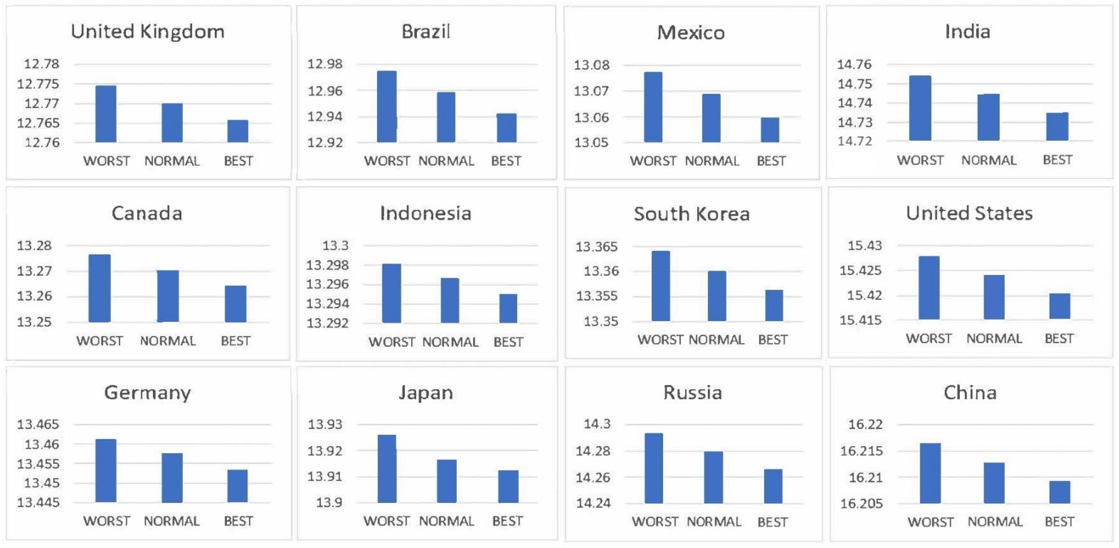
Appendix B. CO2 Emission Forecast Scenarios

There are many different methods of forecasting CO2 emissions available in the literature. The choice of the appropriate method depends on a wide range of factors involved, both qualitatively and quantitatively, due to the different locations and factors of CO2 emissions. Methods based mainly on artificial intelligence, traditional linear regression, computer-aided simulation, scenario analysis, and the optimal development model are popular approaches. In this work, where prediction is not the primary goal, developing scenarios with the help of linear regression was considered the most appropriate technique [119] because we analyzed a large sample of countries where it is problematic to predict all of the determinants (8) used in our analysis to determine carbon dioxide emissions.
In terms of forecasting, we estimated the carbon dioxide emission equation for the period from 1998 to 2019 and determined the estimators of Equation (1):
ΔCO2 = 0.0560095 + (0.5063472*GDPgr) + (−0.0890649*GovExp) + (0.0047487*FDI) +
(−0.0009026*GovEf) + (−0.0240855*M3gr) + (0.0189704*IRmm) + (−0.00214*CBT) +
(−0.0256864*CBI).                                                                                                               
Next, we considered three scenarios with a five-year horizon; in the first (NORMAL), we have a normal emission process. The determinants take the average values of the last five years, and the emissions are calculated from the model equation. In the second scenario (BEST), an improvement of the explanatory variables was calculated by a standard deviation for each factor depending on its contribution to emissions. For example, because GDP contributes aggressively to gas emissions, in the good case scenario, a reduction was calculated by a standard deviation, and the opposite was done for the government efficiency. Finally, the emissions were calculated from the determined Equation (1). In scenario 3 (WORST), we calculated a decrease by a standard deviation for each factor and determined the emissions again based on the equation of our model [120,121,122,123].
This process was performed for the 12 countries with the highest emissions of our sample (>13 thousand metric tons) to have an indicative picture of the most polluted countries. In this process, we included all the determinant variables, except CBT and CBI which show stability in short periods. The signs of the effects of the variables on CO2 emissions are those that emerged from the regressions and specifically: GDPgr (+), GovExp (−), FDI (+), GovEf (−), M3gr (−), and IRmm (+). Table A2 depicts the differences calculated in the amount of carbon dioxide emissions for each scenario and for the countries that emit the most.
Table A2. Differences in the amount of CO2 emissions in three scenarios.
ScenariosNormalBestWorst
Brazil−0.00773−0.023920.008448
Canada0.0092070.0029950.015419
China0.0638820.0602570.067507
Germany−0.01483−0.01878−0.01088
India0.039390.0300140.048767
Indonesia0.0204620.0188850.022038
Japan−0.00015−0.003860.009519
South Korea0.0052470.0012620.009232
Mexico0.003653−0.004980.01229
Russia−0.0108−0.024010.002422
United Kingdom−0.02046−0.02476−0.01616
United States0.00289−0.000850.006632
Several countries appear to be experiencing declining greenhouse gas emissions, such as Brazil, Germany, Japan, Russia, and the United Kingdom. This is due to the significant investments being made in renewable energy sources and because these countries are combining increased GDP and reduced carbon dioxide emissions. However, Germany and the United Kingdom show reduced emissions in all scenarios, even in the worst-case scenario, which means that the downward trend is strong.
Table A3. Total CO2 emissions in thousands of metric tons in three scenarios.
WorstNormalBest
Brazil12.9746512.9584712.94228
Canada13.276513.2702913.26408
China16.2164716.2128416.20922
Germany13.461513.4575413.45359
India14.7540314.7446514.73527
Indonesia13.2981713.2965913.29502
Japan13.9259213.9162513.91253
South Korea13.3640913.360113.35612
Mexico13.0773213.0686813.06005
Russia14.2926414.2794314.26621
United Kingdom12.7743612.7700612.76576
United States15.4278315.4240915.42035
Table A3 shows the countries with the total gas emissions in thousands of metric tons in each scenario. We observe a clear tendency to reduce emissions from the worst to the best scenario, a process in line with the literature [121,124]. In addition, in Figure A1, this trend is evident in each country depending on the level of carbon dioxide emissions.
Figure A1. CO2 emissions of countries with increased emissions under the three scenarios.
Energies 15 04733 g0a1

References

  1. Arent, D.J.; Wise, A.; Gelman, R. The status and prospects of renewable energy for combating global warming. Energy Econ. 2011, 33, 584–593. [Google Scholar] [CrossRef]
  2. Solomon, B.D.; Krishna, K. The coming sustainable energy transition: History, strategies, and outlook. Energy Policy 2011, 39, 7422–7431. [Google Scholar] [CrossRef]
  3. Gielen, D.; Boshell, F.; Saygin, D.; Bazilian, M.D.; Wagner, N.; Gorini, R. The role of renewable energy in the global energy transformation. Energy Strategy Rev. 2019, 24, 38–50. [Google Scholar] [CrossRef]
  4. Pickl, M.J. The renewable energy strategies of oil majors–From oil to energy? Energy Strategy Rev. 2019, 26, 100370. [Google Scholar] [CrossRef]
  5. Spilimbergo, A.; Symansky, S.; Blanchard, O.; Cottarelli, C. Fiscal Policy for the Crisis. In CESifo Forum; IFO Institut für Wirtschaftsforschung an der Universität München: München, Germany, 2009; Volume 10, pp. 26–32. [Google Scholar]
  6. Rosenow, J.; Fawcett, T.; Eyre, N.; Oikonomou, V. Energy efficiency and the policy mix. Build. Res. Inf. 2016, 44, 562–574. [Google Scholar] [CrossRef]
  7. Apergis, N.; Payne, J.E. CO2 emissions, energy usage, and output in Central America. Energy Policy 2009, 37, 3282–3286. [Google Scholar] [CrossRef]
  8. Price, L.; Wang, X.; Yun, J. The challenge of reducing energy consumption of the Top-1000 largest industrial enterprises in China. Energy Policy 2010, 38, 6485–6498. [Google Scholar] [CrossRef]
  9. Dokas, I.; Panagiotidis, M.; Papadamou, S.; Spyromitros, E. The Determinants of Energy and Electricity Consumption in Developed and Developing Countries: International Evidence. Energies 2022, 15, 2558. [Google Scholar] [CrossRef]
  10. Hallerberg, M.; Wolff, G.B. Fiscal institutions, fiscal policy and sovereign risk premia in EMU. Public Choice 2008, 136, 379–396. [Google Scholar] [CrossRef]
  11. Albuquerque, B. Fiscal institutions and public spending volatility in Europe. Econ. Model. 2011, 28, 2544–2559. [Google Scholar] [CrossRef] [Green Version]
  12. Frankel, J.A.; Vegh, C.A.; Vuletin, G. On graduation from fiscal procyclicality. J. Dev. Econ. 2013, 100, 32–47. [Google Scholar] [CrossRef] [Green Version]
  13. McManus, R.; Ozkan, F.G. On the consequences of pro-cyclical fiscal policy. Fisc. Stud. 2015, 36, 29–50. [Google Scholar] [CrossRef]
  14. Calderón, C.; Duncan, R.; Schmidt-Hebbel, K. Do good institutions promote countercyclical macroeconomic policies? Oxf. Bull. Econ. Stat. 2016, 78, 650–670. [Google Scholar] [CrossRef] [Green Version]
  15. Bergman, U.M.; Hutchison, M. Economic stabilization in the post-crisis world: Are fiscal rules the answer? J. Int. Money Financ. 2015, 52, 82–101. [Google Scholar] [CrossRef]
  16. Bergman, U.M.; Hutchison, M.M.; Jensen, S.E.H. Promoting sustainable public finances in the European Union: The role of fiscal rules and government efficiency. Eur. J. Political Econ. 2016, 44, 1–19. [Google Scholar] [CrossRef] [Green Version]
  17. Dutt, K. Governance, institutions and the environment-income relationship: A cross-country study. Environ. Dev. Sustain. 2009, 11, 705–723. [Google Scholar] [CrossRef]
  18. Adams, S.; Klobodu, E.K.M. Urbanization, democracy, bureaucratic quality, and environmental degradation. J. Policy Model. 2017, 39, 1035–1051. [Google Scholar] [CrossRef]
  19. Hosseini, H.M.; Kaneko, S. Can environmental quality spread through institutions? Energy Policy 2013, 56, 312–321. [Google Scholar] [CrossRef]
  20. Wang, Z.; Zhang, B.; Wang, B. The moderating role of corruption between economic growth and CO2 emissions: Evidence from BRICS economies. Energy 2018, 148, 506–513. [Google Scholar] [CrossRef]
  21. Baloch, M.A.; Wang, B. Analyzing the role of governance in CO2 emissions mitigation: The BRICS experience. Struct. Change Econ. Dyn. 2019, 51, 119–125. [Google Scholar]
  22. Zakaria, M.; Bibi, S. Financial development and environment in South Asia: The role of institutional quality. Environ. Sci. Pollut. Res. 2019, 26, 7926–7937. [Google Scholar] [CrossRef]
  23. Campiglio, E.; Dafermos, Y.; Monnin, P.; Ryan-Collins, J.; Schotten, G.; Tanaka, M. Climate change challenges for central banks and financial regulators. Nat. Clim. Change 2018, 8, 462–468. [Google Scholar] [CrossRef]
  24. Monnin, P. Central Banks and the transition to a low-carbon economy. Counc. Econ. Policies Discuss. Note 2018, 1. [Google Scholar] [CrossRef]
  25. Durrani, A.; Rosmin, M.; Volz, U. The role of central banks in scaling up sustainable finance–what do monetary authorities in the Asia-Pacific region think? J. Sustain. Financ. Invest. 2020, 10, 92–112. [Google Scholar] [CrossRef]
  26. Campiglio, E. Beyond carbon pricing: The role of banking and monetary policy in financing the transition to a low-carbon economy. Ecol. Econ. 2016, 121, 220–230. [Google Scholar] [CrossRef] [Green Version]
  27. Polzin, F.; Sanders, M.; Täube, F. A diverse and resilient financial system for investments in the energy transition. Curr. Opin. Environ. Sustain. 2017, 28, 24–32. [Google Scholar] [CrossRef] [Green Version]
  28. Dafermos, Y.; Nikolaidi, M.; Galanis, G. Climate change, financial stability and monetary policy. Ecol. Econ. 2018, 152, 219–234. [Google Scholar] [CrossRef]
  29. Qingquan, J.; Khattak, S.I.; Ahmad, M.; Ping, L. A new approach to environmental sustainability: Assessing the impact of monetary policy on CO2 emissions in Asian economies. Sustain. Dev. 2020, 28, 1331–1346. [Google Scholar] [CrossRef]
  30. Chishti, M.Z.; Ahmad, M.; Rehman, A.; Khan, M.K. Mitigations pathways towards sustainable development: Assessing the influence of fiscal and monetary policies on carbon emissions in BRICS economies. J. Clean. Prod. 2021, 292, 126035. [Google Scholar] [CrossRef]
  31. Noureen, S.; Iqbal, J.; Chishti, M.Z. Exploring the dynamic effects of shocks in monetary and fiscal policies on the environment of developing economies: Evidence from the CS-ARDL approach. Environ. Sci. Pollut. Res. 2022, 29, 45665–45682. [Google Scholar] [CrossRef]
  32. de Mendonça, H.F.; Simão Filho, J. Economic transparency and effectiveness of monetary policy. J. Econ. Stud. 2007, 34, 497–514. [Google Scholar] [CrossRef]
  33. Papadamou, S.; Sidiropoulos, M.; Spyromitros, E. Central bank transparency and the interest rate channel: Evidence from emerging economies. Econ. Model. 2015, 48, 167–174. [Google Scholar] [CrossRef]
  34. Weber, C.S. Central bank transparency and inflation (volatility)–new evidence. Int. Econ. Econ. Policy 2018, 15, 21–67. [Google Scholar] [CrossRef] [Green Version]
  35. Crowe, C.; Meade, E.E. Central bank independence and transparency: Evolution and effectiveness. Eur. J. Political Econ. 2008, 24, 763–777. [Google Scholar] [CrossRef] [Green Version]
  36. Arnone, M.; Romelli, D. Dynamic central bank independence indices and inflation rate: A new empirical exploration. J. Financ. Stab. 2013, 9, 385–398. [Google Scholar] [CrossRef]
  37. Halkos, G.E.; Paizanos, E.A. The effects of fiscal policy on CO2 emissions: Evidence from the USA. Energy Policy 2016, 88, 317–328. [Google Scholar] [CrossRef]
  38. López, R.; Palacios, A. Why has Europe become environmentally cleaner? Decomposing the roles of fiscal, trade and environmental policies. Environ. Resour. Econ. 2014, 58, 91–108. [Google Scholar] [CrossRef]
  39. Yuelan, P.; Akbar, M.W.; Hafeez, M.; Ahmad, M.; Zia, Z.; Ullah, S. The nexus of fiscal policy instruments and environmental degradation in China. Environ. Sci. Pollut. Res. 2019, 26, 28919–28932. [Google Scholar] [CrossRef]
  40. López, R.; Galinato, G.I.; Islam, A. Fiscal spending and the environment: Theory and empirics. J. Environ. Econ. Manag. 2011, 62, 180–198. [Google Scholar] [CrossRef]
  41. Congleton, R.D. Political institutions and pollution control. Rev. Econ. Stat. 1992, 74, 412–421. [Google Scholar] [CrossRef]
  42. Bernauer, T.; Koubi, V. Effects of political institutions on air quality. Ecol. Econ. 2009, 68, 1355–1365. [Google Scholar] [CrossRef]
  43. Ibrahim, M.H.; Law, S.H. Institutional Quality and CO2 Emission–Trade Relations: Evidence from Sub-Saharan Africa. S. Afr. J. Econ. 2016, 84, 323–340. [Google Scholar] [CrossRef]
  44. Abid, M. Impact of economic, financial, and institutional factors on CO2 emissions: Evidence from sub-Saharan Africa economies. Util. Policy 2016, 41, 85–94. [Google Scholar] [CrossRef]
  45. Solarin, S.A.; Al-Mulali, U.; Musah, I.; Ozturk, I. Investigating the pollution haven hypothesis in Ghana: An empirical investigation. Energy 2017, 124, 706–719. [Google Scholar] [CrossRef]
  46. Apergis, N.; Garćıa, C. Environmentalism in the EU-28 context: The impact of governance quality on environmental energy efficiency. Environ. Sci. Pollut. Res. 2019, 26, 37012–37025. [Google Scholar] [CrossRef] [Green Version]
  47. Ozturk, I.; Al-Mulali, U.; Solarin, S.A. The control of corruption and energy efficiency relationship: An empirical note. Environ. Sci. Pollut. Res. 2019, 26, 17277–17283. [Google Scholar] [CrossRef]
  48. Cansino, J.M.; Román-Collado, R.; Molina, J.C. Quality of institutions, technological progress, and pollution havens in Latin America. An analysis of the environmental Kuznets curve hypothesis. Sustainability 2019, 11, 3708. [Google Scholar] [CrossRef] [Green Version]
  49. Hunjra, A.I.; Tayachi, T.; Chani, M.I.; Verhoeven, P.; Mehmood, A. The moderating effect of institutional quality on the financial development and environmental quality nexus. Sustainability 2020, 12, 3805. [Google Scholar] [CrossRef]
  50. Ulucak, R. The pathway toward pollution mitigation: Does institutional quality make a difference? Bus. Strategy Environ. 2020, 29, 3571–3583. [Google Scholar]
  51. Khan, Z.; Ali, S.; Dong, K.; Li, R.Y.M. How does fiscal decentralization affect CO2 emissions? The roles of institutions and human capital. Energy Econ. 2021, 94, 105060. [Google Scholar] [CrossRef]
  52. Liu, X.; Latif, K.; Latif, Z.; Li, N. Relationship between economic growth and CO2 emissions: Does governance matter? Environ. Sci. Pollut. Res. 2020, 27, 17221–17228. [Google Scholar] [CrossRef]
  53. Goel, R.K.; Herrala, R.; Mazhar, U. Institutional quality and environmental pollution: MENA countries versus the rest of the world. Econ. Syst. 2013, 37, 508–521. [Google Scholar] [CrossRef]
  54. Jalil, A.; Feridun, M. The impact of growth, energy and financial development on the environment in China: A cointegration analysis. Energy Econ. 2011, 33, 284–291. [Google Scholar] [CrossRef]
  55. Kaushal, L.A.; Pathak, N. The causal relationship among economic growth, financial development and trade openness in Indian economy. Int. J. Econ. Perspect. 2015, 9, 5–22. [Google Scholar]
  56. Matikainen, S.; Campiglio, E.; Zenghelis, D. The climate impact of quantitative easing. Policy Paper Grantham Research Institute on Climate Change and the Environment. Lond. Sch. Econ. Political Sci. 2017, 36. [Google Scholar] [CrossRef]
  57. Economides, G.; Xepapadeas, A. Monetary Policy under Climate Change (No. 7021). CESifo 2018. [Google Scholar] [CrossRef]
  58. Aslam, B.; Hu, J.; Majeed, M.T.; Andlib, Z.; Ullah, S. Asymmetric macroeconomic determinants of CO2 emission in China and policy approaches. Environ. Sci. Pollut. Res. 2021, 28, 41923–41936. [Google Scholar] [CrossRef]
  59. Chen, C.; Pan, D. The Optimal Mix of Monetary and Climate Policy; MPRA Working Paper No. 97718; MPRA: Munich, Germany, 2020. [Google Scholar]
  60. McKibbin, W.J.; Morris, A.C.; Panton, A.; Wilcoxen, P. Climate Change and Monetary Policy: Dealing with Disruption; Discussion Paper; Brookings Institution: Washington, DC, USA, 2017. [Google Scholar]
  61. Chan, Y.T. Are macroeconomic policies better in curbing air pollution than environmental policies? A DSGE approach with carbon-dependent fiscal and monetary policies. Energy Policy 2020, 141, 111454. [Google Scholar] [CrossRef]
  62. Hajdukovic, I. Interactions among macroeconomic policies, the energy market and environmental quality. Environ. Econ. Policy Stud. 2021, 23, 861–913. [Google Scholar] [CrossRef]
  63. Latief, R.; Lefen, L. Foreign direct investment in the power and energy sector, energy con-sumption, and economic growth: Empirical evidence from pakistan. Sustainability 2019, 11, 192. [Google Scholar] [CrossRef] [Green Version]
  64. Gregorio, J.D. The role of foreign direct investment and natural resources in economic development. In Multinationals and Foreign Investment in Economic Development; Palgrave Macmillan: London, UK, 2005; pp. 179–197. [Google Scholar]
  65. Kaufmann, D.; Kraay, A.; Mastruzzi, M. Governance matters IV: Governance indicators for 1996–2004. World Bank Policy Res. Work. Pap. Ser. 3630 2005. [Google Scholar] [CrossRef] [Green Version]
  66. Eichengreen’s Online Database. Available online: https://eml.berkeley.edu/~eichengr/data.shtml (accessed on 12 March 2022).
  67. Garriga’s Online Database. Available online: https://sites.google.com/site/carogarriga/cbi-data-1 (accessed on 15 March 2022).
  68. World Bank’s Website. Available online: https://info.worldbank.org/governance/wgi (accessed on 12 March 2022).
  69. World Development Indicators Database of the World Bank. Available online: https://databank.worldbank.org/home (accessed on 12 March 2022).
  70. Hafeez, M.; Yuan, C.; Khelfaoui, I.; Sultan Musaad, O.A.; Waqas Akbar, M.; Jie, L. Evaluating the energy consumption inequalities in the one belt and one road region: Implications for the environment. Energies 2019, 12, 1358. [Google Scholar] [CrossRef] [Green Version]
  71. Yan, X.; Crookes, R.J. Energy demand and emissions from road transportation vehicles in China. Prog. Energy Combust. Sci. 2010, 36, 651–676. [Google Scholar] [CrossRef]
  72. Rasoulinezhad, E.; Saboori, B. Panel estimation for renewable and non-renewable energy consumption, economic growth, CO2 emissions, the composite trade intensity, and financial openness of the commonwealth of independent states. Environ. Sci. Pollut. Res. 2018, 25, 17354–17370. [Google Scholar] [CrossRef]
  73. Akbar, M.; Hussain, A.; Akbar, A.; Ullah, I. The dynamic association between healthcare spending, CO2 emissions, and human development index in OECD countries: Evidence from panel VAR model. Environ. Dev. Sustain. 2021, 23, 10470–10489. [Google Scholar] [CrossRef]
  74. Omri, A.; Nguyen, D.K.; Rault, C. Causal interactions between CO2 emissions, FDI, and economic growth: Evidence from dynamic simultaneous-equation models. Econ. Model. 2014, 42, 382–389. [Google Scholar] [CrossRef] [Green Version]
  75. Zhang, C.; Zhou, X. Does foreign direct investment lead to lower CO2 emissions? Evidence from a regional analysis in China. Renew. Sustain. Energy Rev. 2016, 58, 943–951. [Google Scholar] [CrossRef]
  76. Bayar, Y.; Diaconu, L.; Maxim, A. Financial development and CO2 emissions in post-transition European Union countries. Sustainability 2020, 1, 2640. [Google Scholar] [CrossRef] [Green Version]
  77. Isiksal, A.Z.; Samour, A.; Resatoglu, N.G. Testing the impact of real interest rate, income, and energy consumption on Turkey’s CO2 emissions. Environ. Sci. Pollut. Res. 2019, 26, 20219–20231. [Google Scholar] [CrossRef]
  78. Breitenfellner, A.; Pointner, W.; Schuberth, H. The potential contribution of central banks to green finance. Vierteljahrsh. Zur Wirtsch. 2019, 88, 55–71. [Google Scholar] [CrossRef]
  79. De Perthuis, C. Carbon markets regulation: The case for a CO2 central bank. Paris Dauphine Univ. Clim. Econ. Chair Inf. Debates Ser. 2011, 10. [Google Scholar]
  80. Dikau, S.; Ryan-Collins, J. Green Central Banking in Emerging Market an Developing Country Economies; New Economics Foundation: London, UK, 2017. [Google Scholar]
  81. Schoenmaker, D. Greening monetary policy. Clim. Policy 2021, 21, 581–592. [Google Scholar] [CrossRef]
  82. Fischer, S.; Alonso-Gamo, P.; Von Allmen, U.E. Economic developments in the West Bank and Gaza since Oslo. Econ. J. 2001, 111, 254–275. [Google Scholar] [CrossRef]
  83. Gani, A. The relationship between good governance and carbon dioxide emissions: Evidence from developing economies. J. Econ. Dev. 2012, 37, 77. [Google Scholar] [CrossRef]
  84. Im, K.S.; Pesaran, M.H.; Shin, Y. Testing for unit roots in heterogeneous panels. J. Econom. 2003, 115, 53–74. [Google Scholar] [CrossRef]
  85. Choi, I. Unit root tests for panel data. J. Int. Money Financ. 2001, 20, 249–272. [Google Scholar] [CrossRef]
  86. Hausman, J.A. Specification tests in econometrics. Econometrica 1978, 46, 1251–1271. [Google Scholar] [CrossRef] [Green Version]
  87. Wooldridge, J.M. Econometric Analysis of Cross Section and Panel Data; MIT Press: Cambridge, MA, USA, 2010. [Google Scholar]
  88. Drukker, D.M. Testing for serial correlation in linear panel-data models. Stata J. 2003, 3, 168–177. [Google Scholar] [CrossRef]
  89. Greene, W.H. Econometric Analysis, 4th ed.; Prentice Hall, Upper Saddle River: Hoboken, NJ, USA, 2000. [Google Scholar]
  90. Breusch, T.S.; Pagan, A.R. The Lagrange multiplier test and its applications to model specification in econometrics. Rev. Econ. Stud. 1980, 47, 239–253. [Google Scholar] [CrossRef]
  91. Driscoll, J.C.; Kraay, A.C. Consistent covariance matrix estimation with spatially dependent panel data. Rev. Econ. Stat. 1998, 80, 549–560. [Google Scholar] [CrossRef]
  92. Greene, W. Econometric Analysis. Stern School of Business; New York University: New York, NY, USA, 2018. [Google Scholar]
  93. Keele, L.; Kelly, N.J. Dynamic models for dynamic theories: The ins and outs of lagged dependent variables. Political Anal. 2006, 14, 186–205. [Google Scholar] [CrossRef]
  94. Pedroni, P. Fully Modified OLS for heterogeneous cointegrated panels. In Nonstationary Panels 2001 Panel Cointegration, and Dynamic Panels; Emerald Group Publishing Limited: Bingley, UK, 2001. [Google Scholar]
  95. Arouri, M.E.H.; Youssef, A.B.; M’henni, H.; Rault, C. Energy consumption, economic growth and CO2 emissions in Middle East and North African countries. Energy Policy 2012, 45, 342–349. [Google Scholar] [CrossRef] [Green Version]
  96. Salahuddin, M.; Alam, K.; Ozturk, I. The effects of Internet usage and economic growth on CO2 emissions in OECD countries: A panel investigation. Renew. Sustain. Energy Rev. 2016, 62, 1226–1235. [Google Scholar] [CrossRef]
  97. Namahoro, J.P.; Wu, Q.; Zhou, N.; Xue, S. Impact of energy intensity, renewable energy, and economic growth on CO2 emissions: Evidence from Africa across regions and income levels. Renew. Sustain. Energy Rev. 2021, 147, 111233. [Google Scholar] [CrossRef]
  98. Birdsall, N.; Wheeler, D. Trade policy and industrial pollution in Latin America: Where are the pollution havens? J. Environ. Dev. 1993, 2, 137–149. [Google Scholar] [CrossRef]
  99. Zarsky, L. Havens, halos and spaghetti: Untangling the evidence about foreign direct investment and the environment. Foreign Direct Invest. Environ. 1999, 13, 47–74. [Google Scholar]
  100. Jensen, V. The pollution haven hypothesis and the industrial flight hypothesis: Some perspectives on theory and empirics. Cent. Dev. Environ. Work. Pap. 1996, 5. [Google Scholar]
  101. Omri, A.; Daly, S.; Rault, C.; Chaibi, A. Financial development, environmental quality, trade and economic growth: What causes what in MENA countries. Energy Econ. 2015, 48, 242–252. [Google Scholar] [CrossRef] [Green Version]
  102. Maji, I.K.; Habibullah, M.S.; Saari, M.Y. Financial development and sectoral CO2 emissions in Malaysia. Environ. Sci. Pollut. Res. 2017, 24, 7160–7176. [Google Scholar] [CrossRef]
  103. Wang, H.; Dong, C.; Liu, Y. Beijing direct investment to its neighbors: A pollution haven or pollution halo effect? J. Clean. Prod. 2019, 239, 118062. [Google Scholar] [CrossRef]
  104. Box-Steffensmeier, J.M.; Freeman, J.R.; Hitt, M.P.; Pevehouse, J.C. Time Series Analysis for the Social Sciences; Cambridge University Press: Cambridge, UK, 2014. [Google Scholar]
  105. Nguyen, D.K.; Huynh, T.L.D.; Nasir, M.A. Carbon emissions determinants and forecasting: Evidence from G6 countries. J. Environ. Manag. 2021, 285, 111988. [Google Scholar] [CrossRef] [PubMed]
  106. Bokde, N.D.; Tranberg, B.; Andresen, G.B. Short-term CO2 emissions forecasting based on decomposition approaches and its impact on electricity market scheduling. Appl. Energy 2021, 281, 116061. [Google Scholar] [CrossRef]
  107. Dong, F.; Wang, Y.; Su, B.; Hua, Y.; Zhang, Y. The process of peak CO2 emissions in developed economies: A perspective of industrialization and urbanization. Resour. Conserv. Recycl. 2019, 141, 61–75. [Google Scholar] [CrossRef]
  108. Akram, R.; Chen, F.; Khalid, F.; Ye, Z.; Majeed, M.T. Heterogeneous effects of energy efficiency and renewable energy on carbon emissions: Evidence from developing countries. J. Clean. Prod. 2020, 247, 119122. [Google Scholar] [CrossRef]
  109. Bayar, Y.; Sasmaz, M.U.; Ozkaya, M.H. Impact of trade and financial globalization on renewable energy in EU transition economies: A bootstrap panel granger causality test. Energies 2020, 14, 19. [Google Scholar] [CrossRef]
  110. Annicchiarico, B.; Di Dio, F. GHG emissions control and monetary policy. Environ. Resour. Econ. 2017, 67, 823–851. [Google Scholar] [CrossRef] [Green Version]
  111. Hayo, B. Inflation culture, central bank independence and price stability. Eur. J. Political Econ. 1998, 14, 241–263. [Google Scholar] [CrossRef]
  112. Garriga, A.C.; Rodriguez, C.M. More effective than we thought: Central bank independence and inflation in developing countries. Econ. Model. 2020, 85, 87–105. [Google Scholar] [CrossRef]
  113. McConnell, A.; Yanovski, B.; Lessmann, K. Central bank collateral as a green monetary policy instrument. Clim. Policy 2022, 22, 339–355. [Google Scholar] [CrossRef]
  114. Baltagi, B.H. (Ed.) Panel Data Econometrics: Theoretical Contributions and Empirical Applications; Emerald Group Publishing; Elsevier: Oxford, UK, 2006. [Google Scholar]
  115. Costantini, M.; Destefanis, S. Cointegration analysis for cross-sectionally dependent panels: The case of regional production functions. Econ. Model. 2009, 26, 320–327. [Google Scholar] [CrossRef]
  116. Helm, D.; Hepburn, C.; Mash, R. Credible carbon policy. Oxf. Rev. Econ. Policy 2003, 19, 438–450. [Google Scholar] [CrossRef]
  117. Zafar, M.W.; Shahbaz, M.; Hou, F.; Sinha, A. From nonrenewable to renewable energy and its impact on economic growth: The role of research & development expenditures in Asia-Pacific Economic Cooperation countries. J. Clean. Prod. 2019, 212, 1166–1178. [Google Scholar]
  118. Eliet-Doillet, A.; Maino, A.G. Central Banks’ “Green Shift” and the Energy Transition; OIES: Oxford, UK, 2022. [Google Scholar]
  119. Abdullah, L.; Pauzi, H.M. Methods in forecasting carbon dioxide emissions: A decade review. J. Teknol. 2015, 75, 1. [Google Scholar] [CrossRef] [Green Version]
  120. Delarue, E.D.; Luickx, P.J.; D’haeseleer, W.D. The actual effect of wind power on overall electricity generation costs and CO2 emissions. Energy Convers. Manag. 2009, 50, 1450–1456. [Google Scholar] [CrossRef]
  121. Wang, J.; Yang, H.Z.; Lu, Z.B. Prospect of energy-related carbon dioxide emission in China based on scenario analysis. In Proceedings of the 2009 International Conference on Energy and Environment Technology, Guilin, China, 16–18 October 2009; Volume 3, pp. 90–93. [Google Scholar]
  122. Meng, M.; Jing, K.; Mander, S. Scenario analysis of CO2 emissions from China’s electric power industry. J. Clean. Prod. 2017, 142, 3101–3108. [Google Scholar] [CrossRef]
  123. Wang, S.; Zhao, Y.; Wiedmann, T. Carbon emissions embodied in China–Australia trade: A scenario analysis based on input–output analysis and panel regression models. J. Clean. Prod. 2019, 220, 721–731. [Google Scholar] [CrossRef]
  124. Samoilov, I.A.; Nakhutin, A.I. Estimation and medium-term forecasting of anthropogenic carbon dioxide and methane emission in Russia with statistical methods. Russ. Meteorol. Hydrol. 2009, 34, 348–353. [Google Scholar] [CrossRef]
Table 1. Core literature methodologies.
Author(s)Countries Timeframe Method
Baloch and Wang [21]BRICS1997–2017Driscoll-Kraay SE and DOLS
Chan [61]77 countries1980–2000E-DSGE with IRFs
Chishti et al. [30]BRICS1985–2014OLS, FMOLS, DOLS
Dutt [17]94 countries1985–2000OLS (fixed effects panel)
Hajdukovic [62]Switzerland and the UK1990–2016VAR
Halkos and Paizanos [37]The USA1973–2013VAR
Hunjra et al. [49]Pakistan, India, Sri Lanka, Nepal, and Bangladesh1984–2018Panel Regressions
Jalil and Feridun [54]China1953–2006ARDL-ECM
Kaushal and Pathak [55]India1991–2013VAR
Khan et al. [51]Austria, Australia, Belgium, Canada, Germany, Spain, and Switzerland1990–2018CS-ARDL
Lopez and Palacios [38]12 European countries1995–2008Panel fixed effects-TVCE
Lopez et al. [40]38 countries1980–2005Panel fixed/random effects—FSE
Qingquan et al. [29]14 Asian countries1990–2014PFM-LS and PD-LS
Wang et al. [20]BRICS1996–2005Panel Partial LS
Yuelan et al. [39]China1980–2016ARDL
Zakaria and Bibi [22]Bangladesh, India, Pakistan, Sri Lanka, and Nepal1984–20152SLS
Table 2. Descriptive Statistics.
ObsMinMaxMeanMedianStandard DeviationVarianceSkewnessKurtosis
CO2Em20904.24849516.1489610.2578410.521512.2607295.110894−0.03519−0.38329
GHGEm20905.99146516.3295910.8829510.954922.0061944.0248130.058295−0.28004
GDPgr2090−0.205990.3450.0363110.0357410.0385330.0014850.1773357.410194
GovExp20900.0095170.6357930.2709270.2612780.1041460.0108460.299854−0.35547
FDI2090−0.576054.4908280.0641150.0316140.2075970.04309712.7532209.4187
GovEf20902.7292467.4369755.4283975.2846450.9300470.8649880.235591−1.08162
M3gr2090−0.255510.8776130.1125450.0830470.1132490.0128252.0388337.073011
IRmm2090−0.029550.7761680.0584110.040030.0712920.0050832.91928514.91489
CBT2090114.57.2935417.53.31490410.98859−0.00462−1.13759
CBI20900.121630.9040.6193820.60550.200820.040329−0.20415−1.20958
Table 3. Unit-root tests.
IPSADF
CO2Em3.1356
(0.9991)
2.3560
(0.9908)
Δ.CO2Em−21.9815 ***
(0.0000)
−36.5351 ***
(0.0000)
GHGEm3.2179
(0.9994)
2.4274
(0.9924)
Δ.GHGEm−22.3235 ***
(0.0000)
−36.9910 ***
(0.0000)
GDPgr−15.9683 ***
(0.0000)
−22.9885 ***
(0.0000)
GovExp−2.8428 **
(0.0022)
−3.4306 ***
(0.0003)
FDI−11.9641 ***
(0.0000)
−15.9295 ***
(0.0000)
M3gr−14.2447 ***
(0.0000)
−20.4868 ***
(0.0000)
IRmm−10.5815 ***
(0.0000)
−15.5824 ***
(0.0000)
Notes: p-values are in the parentheses. ** and *** indicate statistical significance of at least 95% and 99%, respectively.
Table 4. All countries’ CO2 and GHG emissions.
Dependent ΔCO2 Dependent ΔGHG
FEREDriscoll–KraayGLSFEREDriscoll–KraayGLS
GDPgr0.5010175 ***
(0.000)
0.520761 ***
(0.000)
0.520761 ***
(0.000)
0.520761 ***
(0.000)
0.3498996 ***
(0.000)
0.3473133 ***
(0.000)
0.3473133 ***
(0.000)
0.3473133 ***
(0.000)
GovExp−0.000325
(0.997)
−0.08832 **
(0.012)
−0.08832 ***
(0.000)
−0.08832 **
(0.011)
−0.0105408
(0.852)
−0.0493751 **
(0.017)
−0.0493751 **
(0.009)
−0.0493751 **
(0.016)
FDI0.0051057
(0.753)
0.0040655
(0.761)
0.0040655
(0.426)
0.0040655
(0.760)
0.0052897
(0.580)
0.0029454
(0.708)
0.0029454
(0.405)
0.0029454
(0.708)
GovEf0.0265612 *
(0.077)
−0.0013416
(0.754)
−0.0013416
(0.801)
−0.0013416
(0.753)
0.0055746
(0.529)
−0.0032147
(0.202)
−0.0032147
(0.206)
−0.0032147
(0.201)
M3gr−0.0087763
(0.796)
−0.0244658
(0.403)
−0.0244658
(0.403)
−0.0244658
(0.402)
0.0144446
(0.472)
−0.0043578
(0.801)
−0.0043578
(0.716)
−0.0043578
(0.800)
IRmm0.0118273
(0.862)
0.022801
(0.612)
0.022801
(0.387)
0.022801
(0.611)
−0.0575196
(0.152)
−0.0297584
(0.261)
−0.0297584
(0.269)
−0.0297584
(0.260)
CBT−0.0004853
(0.829)
−0.0020851 *
(0.079)
−0.0020851
(0.115)
−0.0020851 *
(0.078)
0.0002092
(0.874)
−0.0008939
(0.201)
−0.0008939
(0.196)
−0.0008939
(0.200)
CBI0.0038791
(0.951)
−0.02508
(0.121)
−0.02508 **
(0.001)
−0.02508
(0.120)
0.0173733
(0.639)
−0.0170345 *
(0.074)
−0.0170345 **
(0.004)
−0.0170345 *
(0.073)
constant−0.145707
(0.115)
0.0599537 **
(0.013)
0.0599537 **
(0.006)
0.0599537 **
(0.013)
−0.040503
(0.458)
0.0480892 ***
(0.001)
0.0480892 ***
(0.001)
0.0480892 ***
(0.001)
R20.06970.05290.0529 0.03030.06270.0627
Hausman8.33
(0.4018)
9.18
(0.3270)
Wooldridge5.194 **
(0.0249)
14.934 ***
(0.0002)
m-Wald1.7 × 105 ***
(0.0000)
54,895.34 ***
(0.0000)
BP0.00
(1.0000)
0.00
(1.0000)
Notes: p-values are in the parentheses. *, **, and *** indicate statistical significance of at least 90%, 95%, and 99%, respectively.
Table 5. The Root Mean Square Errors of CO2 and GHG emissions for the six regions of the sample (period from 2010 to 2019).
REGIONRMSE_CO2RMSE_GHG
ECA0.0759187610.046356371
MENA0.080768820.041112596
AP0.0767403730.046469136
AME0.0751585050.046223406
WE/EU0.0771241860.04657374
SSA0.0683477860.040114951
ECA: Europe and Central Asia, MENA: the Middle East and North Africa, AP: Asia-Pacific, AME: America and the Caribbean, WE/EU: Western Europe and the European Union, and SSA: Sub-Saharan Africa.
Table 6. Developed countries’ CO2 and GHG emissions.
Dependent ΔCO2 Dependent ΔGHG
FEREDriscoll–KraayGLSFEREDriscoll–KraayGLS
GDPgr0.6697974 **
(0.002)
0.7537896 ***
(0.000)
0.7537896 ***
(0.000)
0.7537896 ***
(0.000)
0.5324164 ***
(0.000)
0.548746 ***
(0.000)
0.548746 ***
(0.000)
0.548746 ***
(0.000)
GovExp−0.0516406
(0.783)
−0.0784817
(0.151)
−0.0784817 *
(0.062)
−0.0784817
(0.138)
−0.0277503
(0.568)
−0.0320581 **
(0.028)
−0.0320581 **
(0.046)
−0.0320581 **
(0.021)
FDI−0.0226092
(0.671)
−0.018778
(0.687)
−0.018778
(0.279)
−0.018778
(0.687)
−0.0120243
(0.383)
−0.0137416
(0.261)
−0.0137416
(0.148)
−0.0137416
(0.255)
GovEf0.0321857
(0.251)
0.004694
(0.486)
0.004694
(0.634)
0.004694
(0.475)
0.0199485 **
(0.006)
−0.0043045 **
(0.016)
−0.0043045 **
(0.030)
−0.0043045 **
(0.009)
M3gr−0.0112305
(0.876)
0.0147909
(0.820)
0.0147909
(0.651)
0.0147909
(0.800)
−0.0057845
(0.757)
−0.0132487
(0.436)
−0.0132487
(0.290)
−0.0132487
(0.400)
IRmm−0.0417223
(0.794)
0.0606893
(0.404)
0.0606893
(0.212)
0.0606893
(0.384)
−0.0604342
(0.146)
0.0057335
(0.767)
0.0057335
(0.622)
0.0057335
(0.716)
CBT−0.0037583
(0.272)
−0.0022123
(0.278)
−0.0022123
(0.198)
−0.0022123
(0.275)
−0.0010417
(0.240)
−0.0010778 **
(0.046)
−0.0010778
(0.117)
−0.0010778 **
(0.037)
CBI0.0336716
(0.760)
−0.0089304
(0.707)
−0.0089304
(0.240)
−0.0089304
(0.696)
0.0011826
(0.967)
−0.0083268
(0.189)
−0.0083268 *
(0.090)
−0.0083268 *
(0.058)
constant−0.177093
(0.355)
−0.0011601
(0.980)
−0.0011601
(0.969)
−0.0011601
(0.969)
−0.1095789 **
(0.027)
0.0409307 ***
(0.001)
0.0409307 **
(0.010)
0.0409307 ***
(0.000)
R20.02190.05100.0510 0.15150.27340.2734
Hausman2.91 (0.9402) 14.92 *
(0.0608)
Wooldridge0.988
(0.3260)
0.690
(0.4109)
m-Wald2.2 × 105 ***
(0.0000)
1273.95 ***
(0.0000)
BP0.27
(0.3004)
0.08
(0.4109)
Notes: p-values are in the parentheses. *, **, and *** indicate statistical significance of at least 90%, 95%, and 99%, respectively.
Table 7. Developing countries’ CO2 and GHG emissions.
Dependent ΔCO2 Dependent ΔGHG
FEREDriscoll–KraayGLSFEREDriscoll–KraayGLS
GDPgr0.4546917 ***
(0.000)
0.4379928 ***
(0.000)
0.4379928 ***
(0.000)
0.4379928 ***
(0.000)
0.2964328 ***
(0.000)
0.2860754 ***
(0.000)
0.2860754 **
(0.003)
0.2860754 ***
(0.000)
GovExp0.0496961
(0.657)
−0.0991773 **
(0.046)
−0.0991773 **
(0.007)
−0.0991773 **
(0.045)
0.017014
(0.846)
−0.0610739
(0.115)
−0.0610739 **
(0.035)
−0.0610739
(0.114)
FDI0.0075242
(0.652)
0.001709
(0.902)
0.001709
(0.694)
0.001709
(0.901)
0.0063487
(0.626)
0.0039227
(0.717)
0.0039227
(0.295)
0.0039227
(0.716)
GovEf0.0176759
(0.324)
−0.0021711
(0.747)
−0.0021711
(0.781)
−0.0021711
(0.746)
−0.0058223
(0.677)
−0.0011362
(0.829)
−0.0011362
(0.861)
−0.0011362
(0.829)
M3gr0.0024391
(0.949)
−0.0301496
(0.351)
−0.0301496
(0.372)
−0.0301496
(0.349)
0.0292892
(0.330)
0.0025029
(0.921)
0.0025029
(0.877)
0.0025029
(0.921)
IRmm0.0354094
(0.632)
0.0112998
(0.850)
0.0112998
(0.797)
0.0112998
(0.849)
−0.0490621
(0.396)
−0.0503946
(0.280)
−0.0503946
(0.317)
−0.0503946
(0.278)
CBT0.0032285
(0.299)
0.0001181
(0.947)
0.0001181
(0.926)
0.0001181
(0.947)
0.0023592
(0.330)
−0.0006313
(0.652)
−0.0006313
(0.536)
−0.0006313
(0.651)
CBI−0.0132635
(0.861)
−0.0516529 **
(0.041)
−0.0516529 **
(0.003)
−0.0516529 **
(0.040)
0.0272399
(0.645)
−0.0263021
(0.184)
−0.0263021 **
(0.048)
−0.0263021
(0.182)
constant−0.1077269
(0.284)
0.0776734 **
(0.020)
0.0776734 **
(0.011)
0.0776734 **
(0.019)
−0.0043257
(0.956)
0.0469473 *
(0.072)
0.0469473
(0.108)
0.0469473 *
(0.071)
R20.12140.04820.0482 0.05840.03450.0345
Hausman7.93
(0.4401)
6.34
(0.6093)
Wooldridge4.613 **
(0.0365)
14.828 ***
(0.0003)
m-Wald13397.25 ***
(0.0000)
20262.14 ***
(0.0000)
BP0.00
(1.0000)
0.00
(1.0000)
Notes: p-values are in the parentheses. *, **, and *** indicate statistical significance of at least 90%, 95%, and 99%, respectively.
Table 8. All countries’ CO2 and GHG emissions under FMOLS.
Dependent ΔCO2Dependent ΔGHG
FMOLSFMOLS
GDPgr0.5063472 ***
(0.000)
0.3362639 ***
(0.000)
GovExp−0.0890649 ***
(0.000)
−0.0521193 **
(0.018)
FDI0.0047487
(0.299)
0.0033989
(0.682)
GovEf−0.0009026
(0.542)
−0.0027072
(0.313)
M3gr−0.0240855 **
(0.016)
−0.0029406
(0.872)
IRmm0.0189704
(0.221)
−0.0297835
(0.289)
CBT−0.00214 ***
(0.000)
−0.0008483
(0.255)
CBI−0.0256864 ***
(0.000)
−0.0160313
(0.111)
constant0.0560095 ***
(0.000)
0.0457302 **
(0.004)
linear3.15 × 10−6 *
(0.065)
2.93 × 10⁻⁷
(0.925)
R20.028210.0180115
Notes: p-values are in the parentheses. *, **, and *** indicate statistical significance of at least 90%, 95%, and 99%, respectively. In FMOLS, the linear eqtrend effects are controlled (1).
Publisher’s Note: MDPI stays neutral with regard to jurisdictional claims in published maps and institutional affiliations.

