Abstract
A permanent magnet actuator (PMA) is a critical device for transforming, transmitting, and protecting electrical energy in renewable energy systems. The reliability of a PMA exerts a direct effect on the operational safety, stability, and reliability of renewable energy systems. An effective fault diagnosis and adjustments for manufacturing processes (MPs) are vital for improving the reliability of a PMA. However, the state-of-the-art fault diagnosis methods are mainly used for single process parameters, extensive sample data, and automated manufacturing systems under real-time monitoring and are not applicable to a PMA with low levels of automation and high human factor-induced uncertainties. This study proposes a novel fault diagnosis approach based on a surrogate model and machine learning for multiple manufacturing processes of a PMA with insufficient training data due to human factor uncertainties. First, a surrogate model that correlated the MP parameters with the output characteristics (OCs) was constructed by a finite element simulation. Second, the quality performance of the OCs under different fault combinations with the mean or variance of the shift of the MP parameters as typical patterns was calculated by the Monte Carlo method. Finally, using the above computations as the training data, a fault diagnosis model capable of identifying the fault pattern of the manufacturing process parameters according to the OCs was constructed based on machine learning. This approach compensated for the inadequacies of traditional fault diagnosis methods with complex analytical models or numerous processing data. The effectiveness and potential applications of the proposed approach were verified through a case study of a rotary PMA in smart grids.
1. Introduction
Electrical energy is essential for human production and management activities. At this stage, the development and utilization of electrical energy are plagued by two major contradictions; one is between the increasing electrical energy demand and the depletion of traditional fossil energy (e.g., oil, gas, and coal), and the other is between the accumulated environmental pressure and the high-emission energy consumption structure [1,2]. The International Energy Agency has predicted that global energy demand will grow by 50% to 60% by 2030, with emerging markets such as Asia, South America, and Africa being the main drivers of global energy demand growth in the future, especially Southeast Asia, where energy consumption is predicted to grow at an annual rate of around 6% [3]. In this context, it is a priority to achieve a smooth and efficient energy transition based on new energy sources (such as wind, solar, and hydropower) and to accelerate this transition, thus achieving energy security and the goal of a carbon peak as well as carbon neutrality [4,5].
Photovoltaic generation, wind generation, biomass and hydropower generation, and electric vehicle applications, for example, can effectively address the non-renewability and environmental pollution induced by traditional fossil energy. The past few decades have seen successes in related pioneering technologies, even in large-scale applications [6]. With the increase in renewable energy generation, conversion, and transmission, the safety and reliability of renewable electricity energy caused by randomness and volatility cannot be ignored. Power electronics are the basis and key to the security, reliability, and stability of renewable power energy systems. Permanent magnet actuators (PMAs), although one of the least reliable components of power electronics [7,8], are widely used in smart grids, photovoltaic generation facilities, electric vehicles, and all-electric aircraft (an example is shown in Figure 1), and play a role in circuit conversion and safety protection, for example [9,10]. Current research focuses on the design and optimization of PMAs whilst ignoring the influence of the manufacturing processes (MPs) on the reliability of the PMA [11,12]. The MP is one of the leading factors affecting the PMA lifecycle [13]. As it becomes increasingly complicated and diversified, fault diagnoses and optimization according to relevant information and data have become indispensable measures to improve the reliability of PMAs and have attracted much research attention [14,15].
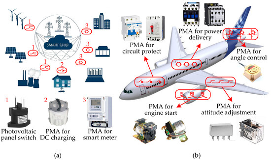
Figure 1.
Typical applications of a PMA in renewable energy systems: (a) PMAs in smart grids (1: power generation; 2: power distribution; 3: signal measurement); (b) PMAs in all-electric aircraft.
The batch production of PMAs comprises a large number of parts; the MP covers multiple stages such as machining, heating, welding, coating, cleaning, assembling, adjustments, encapsulating, and baking. The manufacturing process parameters are used to characterize the process quality. The complexity of MMPs and an abnormal variation in the MP parameters inevitably cause unit-to-unit variability, resulting in a poor qualified rate and poor reliability in the batch production [16,17,18]. Therefore, it is imperative to conduct an effective fault diagnosis of MPs and resolve the abnormal variation sources. Generally, the main fault diagnosis methods for MPs can be divided into data-driven and model-based approaches. The former requires abundant historical and online detection data, deploying artificial intelligence algorithms. The latter is based on the knowledge of the diagnosed system that can be obtained from the physical principles, the fault mechanisms, and relevant expertise, for example [19,20]. Studies on the fault diagnosis of aircraft maintenance, semiconductor manufacturing, and spur gear revealed the effectiveness of the two methods [21,22,23].
Current manufacturing trends veer towards multi-variety and small-batch production [24], making it increasingly difficult to obtain substantial data, especially fault data. Moreover, as mentioned above, complex product structures and MPs make the requisite manufacturing systems-relevant knowledge inaccessible. Traditional fault diagnosis methods cannot address these issues. The development of computer simulation technology can ensure accessible output characteristics (OCs) through numerical methods such as finite element, finite difference, and matrix methods. The simulation model was identified to present the influence of the MPs easily and precisely [25,26,27,28]. However, model complexities entail high computational costs. One effective solution is the use of surrogate models.
Surrogate models, also known as approximation models, are used to represent a complex phenomenon and have gained increasing popularity over past decades due to their ability to exploit the black-box nature of the problem and their attractive computational simplicity [29]. A surrogate model acts as a model of a model and, thus, can replace an expensive simulation model by approximating its input–output responses. There are many commonly used surrogate modeling methods such as a polynomial response surface, neural networks, Kriging, radial basis functions, Bayesian networks, and random forests [30]. The preparation of an accurate surrogate model necessitates adequate simulation sample points. Appropriate experimental design methods can reduce this number of training sample points, thus shortening the simulation time [31,32].
Surrogate models provide an accurate and efficient data source for reliability assessments and optimization. Existing MP diagnosis methods mainly rely on historical fault data and experiments. These methods are unsuitable for the fault diagnosis for the MP of PMAs in small batches and multiple varieties. In this paper, we propose a new method of fault diagnosis in the manufacturing process. For the first time, surrogate modeling theory is introduced into constructing the sample database required for the MP diagnosis model training. Combined with the machine learning method, we solve the problem of data sources and a multiple fault coupling diagnosis. Based on this, we propose a novel fault diagnosis approach for the MPs of PMAs. Section 2 introduces the basic flow of the proposed approach, the surrogate model building, the training data calculation, and the fault diagnosis process. Section 3 presents the case study, in which a rotary PMA is chosen as an example to verify the effectiveness of the proposed approach. Section 4 conveys the concluding remarks.
2. The Proposed Fault Diagnosis Approach for the MPs of PMAs
2.1. Procedure of the Proposed Approach
Figure 2 illustrates the proposed fault diagnosis approach for the MPs of PMAs for renewable energy systems. The critical processes of the proposed approach were as follows: (a) the construction of the surrogate model of the MP parameters and the OCs; (b) the calculation of the training data under different fault patterns; and (c) the construction of the fault diagnosis model of the MPs.
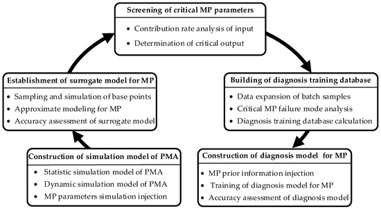
Figure 2.
Procedure of the proposed approach.
The simplified procedure for the fault diagnosis of the MPs for PMAs based on the surrogate model was as follows:
- (a)
- A simulation model of a PMA was constructed based on the MP data. Statistic and dynamic OCs were calculated by the model. The key MP parameters and OCs were selected. The MP parameters were injected.
- (b)
- An approximate modeling method was chosen considering the number of simulated sample points used for the surrogate model construction. The accuracy of the surrogate model was evaluated through the corresponding indexes.
- (c)
- The MP parameters significantly influencing the consistency of the OCs were further identified by the contribution rate analysis method. The critical OCs were determined according to the system requirements.
- (d)
- Based on a critical MP failure mode analysis, the means and variances of the key OCs of a batch of products under different combinations were obtained through statistics from the corresponding computational results.
- (e)
- An appropriate fault diagnosis model was chosen and trained by the constructed database. The prior information of the MP was used to optimize the model parameters. Its accuracy was assessed by the appropriate indexes.
2.2. Simulation Modeling and the MP Parameter Injection of the PMAs
The simulation of PMA OCs is an electromechanical coupling process, including both the static magnetic chains and suction calculation as well as the dynamic electromagnetic force of the electromagnetic and mechanical system, posing challenges to solving the problem in single commercial software. In this paper, we proposed a joint simulation modeling method using the software of 3D modeling, an electromagnetic field analysis, and a dynamics analysis. The modeling process is shown in Figure 3. The proposed model included the following two aspects for the PMA.
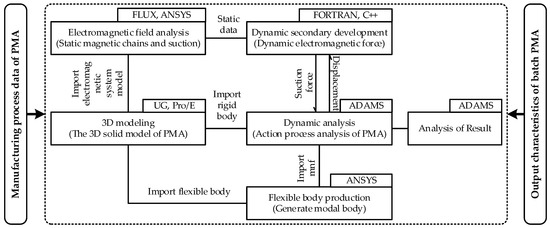
Figure 3.
The simulation modelling procedure of the PMA.
- (a)
- The calculation model of static OCs: The 3D modeling software UG and Pro/E were used to establish the PMA 3D solid model. The corresponding solid model was imported into the software for the dynamics analysis, flexible body generation, and the electromagnetic field analysis. A data interface between the software and the rigid and flexible body was generated to carry out the electromagnetic characteristics research. The rigid and flexible bodies were positioned and assembled in the dynamics software to establish a complete mechanical system dynamic model.
- (b)
- The calculation model of dynamic OCs: The loading of dynamic electromagnetic forces and the simulation of the dynamic characteristics of the PMA were performed through the secondary development of the dynamics software. In the post-processing (e.g., ADAMS), the corresponding results were extracted and analyzed after the simulation. One merit of this method was that it combined multiple software programs and gave full play to the advantages of each type of software. The disadvantage was that each time step during the dynamic simulation required the secondary development module to read and write to a disk file, decelerating the simulation.
- (c)
- MP parameter injection and analysis: The manufacturing process data of the PMA were injected into the simulation model and the output characteristics of the current manufacturing state were calculated. At the same time, the degree of influence of the manufacturing process fluctuations on the output characteristics of the PMA was analyzed according to the quality requirements and the critical MP parameters were screened out to lay the foundation for the establishment of the surrogate model of the PMA.
2.3. The Establishment of a Surrogate Model for the MP
Based on the screened critical manufacturing processes, the sample points (a series of virtual prototypes) within the allowed range of MP parameters of the PMA were generated by Latin hypercube sampling (LHS), orthogonal experimental design (OED), or uniform sampling (US); thus, a simulation model was obtained for the OCs of each prototype.
For example, the mathematical model for calculating the dynamic characteristics of a PMA with a rotating armature motion is shown in Equation (1), which contains the differential equation for the coil, the motion equation for the movable components (armature), and the differential equation for the angular velocity and angular displacement.
where ψ and U are the flux and voltage of the PMA control coil, respectively; i and R are the current and resistance of the PMA control coil, respectively; α and ω are the angular displacement and angular velocity of the movable component (armature), respectively; J is the kinetic energy of the movable component (armature) rotation; Mx is the suction torque; Mf is the counter torque; and ψ0 and α0 are the coil flux and armature displacement at t = 0, respectively.
The dynamic equations of the PMA in Equation (1) could be calculated quickly and accurately. In contrast, for the electromagnetic field equations—especially for the 3D electromagnetic systems—the solution speed of the inefficient finite element significantly reduced the efficiency of the performance analysis of the electromechanical component products. Therefore, we built an alternative model for electromagnetic systems based on custom interpolation functions.
The basic form of the PMA electromagnetic suction torque model is expressed in Equation (2), assuming that the perturbations induced by the parameter changes did not affect each other.
where F is the static suction torque; F0 is the suction torque with the MP parameters unchanged; and ΔFi is the static suction torque disturbance caused by fluctuations in each MMP xi and can be obtained through interpolation.
A function was then defined: f = g(x1, x2), for [m − Δx1, m, m + Δx1]⊂X1, [n − Δx2, n, n + Δx2]⊂X2, (Δx1, Δx2 > 0). When f was monotonic for both Δx1 and Δx2, then g(m, n) was between the points g(m − Δx1, n − Δx2), g(m + Δx1, n − Δx2), g(m − Δx1, n + Δx2), and g(m + Δx1, n + Δx2), as shown in Figure 4.
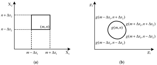
Figure 4.
The relationship of design parameters and function range: (a) design parameter range; (b) function range.
Therefore, g(m, n) could be expressed as:
where l is the weight coefficient of each point, indicating the influence of each point on the target point. Two conditions were required to be met simultaneously: (a) when the output value was the node value, the weight coefficient of the node was 1 and the other points were 0; and (b) the value range of the weight coefficient was 0 ≤ l ≤1.
The OCs of the electromagnetic suction torque of the PMA satisfied the monotonicity with respect to the voltage and rotation angle if four boundary points were chosen; i.e., (Um0, αn0), (Um1, αn0), (Um0, αn1), and (Um1, αn1). (Um0 ≤ U ≤ Um1, αm0 ≤ α ≤ αm1), which could be obtained from Equation (4) as follows:
where h(U, α) is the interpolation function.
The model with the optimum common evaluation index of model accuracy (RMSE) was then assessed as follows:
where ntest is the number of selected test samples and is the actual response value of the test sample points; i.e., the simulation value. is the predicted value of the surrogate model. A poor RMSE reflected a high model accuracy.
When the model accuracy failed to meet the requirements, it could be enhanced by increasing the sample points. The surrogate modeling process is shown in Figure 5.
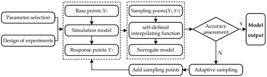
Figure 5.
Procedure of the surrogate model construction.
2.4. The Screening of the Critical Parameters
The contribution rate analysis method is a statistical method for experimental data that identifies the main factors affecting the MP of the PMA from numerous MP parameters. The calculation and analysis of the contribution rate for the multi-factor non-replicated experiments are shown in Table 1.

Table 1.
Calculation and analysis of the contribution rate of multiple design parameters.
Using a 6-factor 3-level experiment as an example, the contribution margin analysis is shown in Equations (6)–(13) [9].
where Sil and Siq are the fluctuation of the squared primary term and the squared quadratic term of the controllable factor xi corresponding with the OC y, respectively. Se is the sum of the squared error terms, Ve is the error variance, and dfe is the degree of freedom of the error term. If a term smaller than Ve existed in Sil and Siq, it was subsumed into Se. For each subsumed term, dfe was added to by 1. T1i, T2i, and T3i were the partial sums of the test results corresponding with three levels of the test factor xi, respectively, and expressed as follows:
where ρil and ρiq are the contribution rate of the primary and quadratic terms of the parameter xi corresponding with the OC y, respectively; ρe is the error term contribution rate.
2.5. The Building of the Diagnosis Training Database
A variation in a few of the MP parameters after the preliminary screening had a slight effect on the output characteristics. The set of key MP parameters that influenced the variation in the OCs (e.g., the qualified rate of the PMA) was gained by the contribution rate analysis method and expressed as XK = {xk1, xk2, …, xkn}. According to the analysis of the normal manufacturing process data, the central value and tolerance sets corresponding with these key manufacturing process parameters were μK = {μk1, μk2, …, μkn} and σK = {σk1, σk2, …, σkn}, respectively.
As the ith key MPP (xki) complied with the measured data of N(μki, σki), a few data were expanded into the batch data through the Monte Carlo method and the MP parameters were randomly combined. The key OCs of each individual were gained by the surrogate model. Finally, a statistical analysis of the OCs of a batch product was undertaken, through which the quality performance of a normal MP was calculated (e.g., the mean, variance, and qualified rate). The procedure is shown in Figure 6.
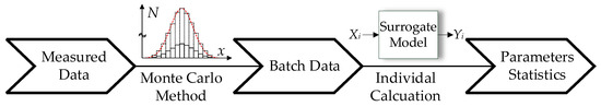
Figure 6.
Procedure of the calculation of the quality performance.
Faults were injected into the mean or variance of the manufacturing process parameters to simulate possible parameter shifts during actual manufacturing. Similarly, the Monte Carlo method and the constructed surrogate model obtained a quality performance under various fault patterns. When the mean or variance was within the shift range of a particular fault pattern, a certain number of samples were chosen for the statistical analysis and quality performance computation. The fault patterns of the manufacturing process parameters for the PMA are shown in Table 2.
Table 2.
Fault patterns of MP parameters. (“↑” means increase, “↓” means decrease).
2.6. Fault Diagnosis for the MPs Based on Machine Learning
Different MP parameters can affect the OCs of PMAs and even directly trigger PMA functional failure. In order to monitor the performance of the PMA through its MP parameters, we adopted a BP neural network model to establish a non-linear mapping relationship between the MP parameters and the health status to achieve a fault diagnosis for the MPs of the PMA. The specific implementation is shown in Figure 7.
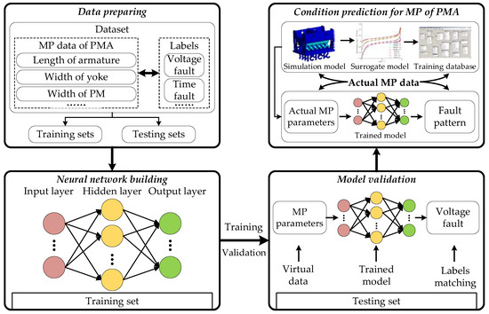
Figure 7.
Fault diagnosis of the manufacturing process.
First, the data set was constructed by combining the MP parameters according to the PMA, with each group including the armature length, armature width, yoke length, yoke step height, permanent magnet width, and core diameter. The simulation model obtained the static and dynamic OCs corresponding with each group of process parameters and used them as labels for the group. The data set was then randomly sampled, with 20% taken as the test set and the remaining 80% as the training set.
Afterward, the neural network was constructed. The number of neurons in the input and output layers was determined according to the dimension of MP parameters and output features. Two fully connected layers were set up as hidden layers in between. Finally, the neural network was activated with a sigmoid function. The MP parameters and labels from the training set were then fed into the input and output layers of the neural network for training. The overall architecture is shown in Figure 8.
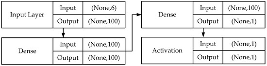
Figure 8.
The overall architecture of the neural network.
Subsequently, the trained model was validated using a test set. When the model achieved a prediction with the required accuracy, new MP parameters could be input into the model and whether the OCs met the thresholds could be observed to predict the health and fault status of the PMA.
The accuracy of the classifier and prediction was evaluated through the corresponding evaluation indexes. The diagnostic accuracy is shown in Equation (14).
where NC is the number of accurately classified samples and N is the total sample size.
3. Case Study
We selected a rotary PMA with a double permanent magnet configuration as the case; the physical prototype electromagnetic, and contact system are shown in Figure 9. The rotated angle was 0–2° and the rated coil voltage was 28 V. The time and voltage of suction and release did not exceed 2 ms and 14 V, respectively.
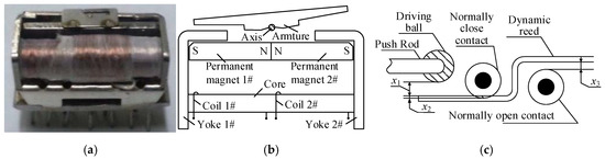
Figure 9.
The rotary PMA with a double permanent magnet: (a) physical prototype; (b) electromagnetic system; (c) contact system.
Using the PMA simulation modeling method, the machine model was first established in UG. The model was imported into ANSYS and the electromagnetic suction torque curve was calculated. The multi-body dynamics simulation software ADAMS was used for the simulation analysis of the reaction force characteristics of the contact spring system. Simulink was utilized to establish the calculation module of the coil circuit and the interpolation module of the electromagnetic torque and current. The mechanical system model established by ADAMS was embedded into the model established by Simulink as a submodule to address the dynamics problems. The dynamic characteristic analysis of Simulink and ADAMS was interactively completed; the model is partially shown in Figure 10.
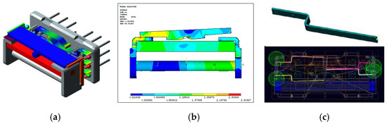
Figure 10.
The simulation model of a rotary PMA: (a) 3D model of the entire machine; (b) electromagnetic system simulation model; (c) contact system simulation model.
Using the PMA simulation model, the OCs (such as the coil current waveform and the suction and release time of the PMA) were calculated. The results are shown in Figure 11.
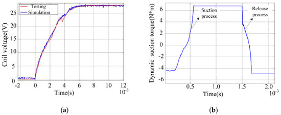
Figure 11.
The simulation results of the rotary PMA: (a) coil voltage; (b) dynamic suction and release output characteristics.
According to the comparison of the simulation results of the coil voltage during the PMA suction with the measured results, the error between the measured and simulated values was within 5%, which verified the accuracy of the simulation model.
Based on the working principle and simulation results of the PMA, there were six main manufacturing process parameters for the PMA. The parameter names, central values, and variances are shown in Table 3.
Table 3.
Critical MP parameters.
A simulation model of the PMA was constructed. The variation range of the critical MP parameters was set as ±12% of the central value. Later, 90 groups of simulation sample points were chosen by LHS and brought into the simulation model to obtain corresponding OCs. A surrogate model of the MP parameters and OCs was constructed through custom interpolation functions based on these sampling points. An additional ten random samples were selected to verify the accuracy of the model. The comparison results of the surrogate and simulation models are shown in Figure 12.
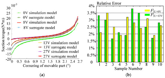
Figure 12.
The comparison of the surrogate model with the simulation model: (a) static output characteristics (suction torque); (b) dynamic output characteristics (operation voltage and operation time).
As shown in Figure 11, the relative computational error was lower than 4%. The RMSE of the model was calculated according to Equation (5).
The surrogate model had high accuracy, meeting the requirement of fault diagnosis for the MPs.
The set of parameters significantly affecting the output variation could be gained through the contribution rate analysis method and expressed as XK = {x1, x2}.
Based on an actual manufacturing investigation, possible fault patterns of these two manufacturing process parameters were disclosed; the variation range was then determined. Training samples for the fault diagnosis model were obtained according to the above method. The results are shown in Table 4.
Table 4.
Fault pattern and related parameters. (“↑” means increase, “↓” means decrease).
By analyzing the working principle of the PMA, three key OCs that reflected the characteristics that customers are most concerned about were selected as the fault features. Specifically, the pick voltage (U3, feature 1) could reflect the working efficiency of the PMA and the release and pick time (t1 and t2, feature 1 and feature 2, respectively) could reflect the operating sensitivity of the PMA. The corresponding physics working process of the PMA is shown in Figure 13. The training samples were classified through the introduced machine learning method. The relevant parameters or the fault characteristics during machine learning were chosen and adjusted. The final classification results are shown in Figure 14.
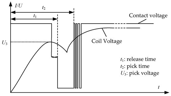
Figure 13.
Selected features according to the physics working process of the PMA.
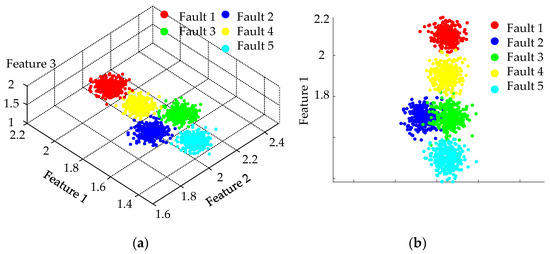
Figure 14.
The diagnosis result: (a) final classification results; (b) the necessity for feature 3.
Similarly, the diagnostic accuracy of the model could be calculated from the classification results of the testing samples:
As can be observed, the model presented high accuracy and could meet the engineering application requirements.
The corresponding fault features were brought into the fault diagnosis model from the quality performance of the aerospace relay manufacturing process with a low qualified rate. Based on the statistical analysis, the variance in the MP parameters increased corresponding with the diagnosed fault pattern in response to cutting tool wear, thus significantly decreasing the suitable rate. The proposed method was verified using an actual case.
4. Conclusions
The reliability of the MP exerts a direct influence on the PMA product quality. In this study, we proposed a new fault diagnosis approach for the MPs of a PMA based on a surrogate model and machine learning method to address the issues of the single process parameters and real-time data requirements that are plagued by traditional diagnostic methods. The following results and contributions were achieved.
- (1)
- The simulation and surrogate modeling methods of static and dynamic OCs were proposed for the fault diagnosis of the MPs. Machine learning was then introduced into the fault diagnosis and a comprehensive diagnosis of multiple faults of the manufacturing process was achieved. Taking the rotary PMA as an example, the simulation and surrogate model error was no greater than 5% and the fault diagnosis accuracy was over 92%.
- (2)
- A surrogate model of the MP parameters and the product output characteristics was built based on finite element simulations with no stipulations for copious knowledge reserves on the complicated MP or relative data. This is a new method for obtaining training data for fault diagnoses.
- (3)
- Many factors such as material attributes, tool wear, and assembly quality have not been previously considered and diagnosed due to the complexity of MPs. The approach proposed here considered the comprehensive influences of the MP parameters on the product quality through a finite element simulation. This offers a new direction in MP optimization.
- (4)
- Considering the key MP parameters determined in this method, it demonstrates a certain relevance for monitoring MPs or lowering the involved costs. The proposed fault diagnosis approach for MPs requires no prior conditions. It can accept multiple MP parameters and is convenient to implement.
Author Contributions
Conceptualization, H.C. and J.T.; methodology, J.T.; software, J.T.; validation, H.C., J.T., and Y.L.; formal analysis, J.T.; investigation, Y.L.; resources, H.C.; data curation, J.T.; writing—original draft preparation, J.T.; writing—review and editing, X.Y.; visualization, X.Y.; supervision, X.Y.; project administration, X.Y.; funding acquisition, Y.L. All authors have read and agreed to the published version of the manuscript.
Funding
This research was funded by the Plan Project of Wenzhou Municipal Science and Technology, Wenzhou University, grant number G20210030.
Institutional Review Board Statement
Not applicable.
Informed Consent Statement
Not applicable.
Data Availability Statement
Not applicable.
Conflicts of Interest
The authors declare no conflict of interest.
References
- Hernandez-Alvidrez, J.; Darbali-Zamora, R.; Flicker, J.D.; Shirazi, M.; Vander Meer, J.; Thomson, W. Using Energy Storage-Based Grid Forming Inverters for Operational Reserve in Hybrid Diesel Microgrids. Energies 2022, 15, 2456. [Google Scholar] [CrossRef]
- Araujo, W.R.H.; Reis, M.R.C.; Wainer, G.A.; Calixto, W.P. Efficiency Enhancement of Switched Reluctance Generator Employing Optimized Control Associated with Tracking Technique. Energies 2021, 14, 8388. [Google Scholar] [CrossRef]
- Chu, W.; Vicidomini, M.; Calise, F.; Duić, N.; Østergaard, P.A.; Wang, Q.; da Graça Carvalho, M. Recent Advances in Low-Carbon and Sustainable, Efficient Technology: Strategies and Applications. Energies 2022, 15, 2954. [Google Scholar] [CrossRef]
- Zhao, S.; Ding, L.; Ruan, Y.; Bai, B.; Qiu, Z.; Li, Z. Experimental and Kinetic Studies on Steam Gasification of a Biomass Char. Energies 2021, 14, 7229. [Google Scholar] [CrossRef]
- Lu, X.; Chan, K.; Xia, S.; Shahidehpour, M.; Ng, W. An Operation Model for Distribution Companies Using the Flexibility of Electric Vehicle Aggregators. IEEE Trans. Smart Grid 2021, 12, 1507–1518. [Google Scholar] [CrossRef]
- Li, J.; Chen, J.; Guo, H. Triboelectric Nanogenerators for Harvesting Wind Energy: Recent Advances and Future Perspectives. Energies 2021, 14, 6949. [Google Scholar] [CrossRef]
- Long, B.; Liao, Y.; Chong, K.T.; Rodríguez, J.; Guerrero, J.M. Enhancement of Frequency Regulation in AC Microgrid: A Fuzzy-MPC Controlled Virtual Synchronous Generator. IEEE Trans. Smart Grid 2021, 12, 3138–3149. [Google Scholar] [CrossRef]
- Lin, J.; Zhao, Y.; Zhang, P.; Wang, J.; Su, H. Research on Compound Sliding Mode Control of a Permanent Magnet Synchronous Motor in Electromechanical Actuators. Energies 2021, 14, 7293. [Google Scholar] [CrossRef]
- Hatzakis, T.; Rodrigues, R.; David, W. Smart Grids and Ethics. ORBIT J. 2019, 2, 1–28. [Google Scholar]
- Noriko, M.; Michiya, T.; Hitoshi, O. Moving to an All-Electric Aircraft System. IHI Eng. Rev. 2014, 47, 33–39. [Google Scholar]
- Ye, X.; Chen, H.; Chen, C.; Zhai, G. Life-Cycle Dynamic Robust Design Optimization for Batch Production of Permanent Magnet Actuator. IEEE Trans. Ind. Electron. 2021, 68, 9885–9896. [Google Scholar] [CrossRef]
- Jiang, J.; Lin, H.; Fang, S. Multi-Objective Optimization of a Permanent Magnet Actuator for High Voltage Vacuum Circuit Breaker Based on Adaptive Surrogate Modeling Technique. Energies 2019, 12, 4695. [Google Scholar] [CrossRef] [Green Version]
- Ye, X.; Chen, H.; Sun, Q.; Chen, C.; Niu, H.; Zhai, G.; Li, W.; Yuan, R. Life-cycle Reliability Design Optimization of High-power DC Electromagnetic Devices Based on Time-dependent Non-probabilistic Convex Model Process. Microelectron. Reliab. 2020, 114, 113795. [Google Scholar] [CrossRef]
- Qiao, L.; Kao, S.; Zhang, Y. Manufacturing Process Modelling Using Process Specification Language. Int. J. Adv. Manuf. Technol. 2011, 55, 549–563. [Google Scholar] [CrossRef]
- Yan, J.; Meng, Y.; Lu, L.; Li, L. Industrial Big Data in an Industry 4.0 Environment: Challenges, Schemes, and Applications for Predictive Maintenance. IEEE Access 2017, 5, 23484–23491. [Google Scholar] [CrossRef]
- Ye, X.; Lin, Y.; Wang, Q.; Liu, H.; Zhai, J. Manufacturing Process-based Storage Degradation Modelling and Reliability Assessment. Microelectron. Reliab. 2018, 88, 107–110. [Google Scholar] [CrossRef]
- Deng, J.; Liu, X.; Zhai, G. Robust Design Optimization of Electromagnetic Actuators for Renewable Energy Systems Considering the Manufacturing Cost. Energies 2019, 12, 4353. [Google Scholar] [CrossRef] [Green Version]
- Ye, X.; Deng, J.; Wang, Y.; Zhai, G. Quality Analysis and Consistency Design of Electromagnetic Device Based on Approximation Model. IEEE Trans. Compon. Packag. Manuf. Technol. 2015, 5, 99–107. [Google Scholar]
- Xu, Y.; Sun, Y.; Wan, J.; Liu, X.; Song, Z. Industrial Big Data for Fault Diagnosis: Taxonomy, Review, and Applications. IEEE Access 2017, 5, 17368–17380. [Google Scholar] [CrossRef]
- Yu, M.; Xiao, C.; Jiang, W.; Yang, S.; Wang, H. Fault Diagnosis for Electromechanical System via Extended Analytical Redundancy Relations. IEEE Trans. Ind. Inform. 2018, 14, 5233–5244. [Google Scholar] [CrossRef]
- Yao, Q.; Wang, J.; Zhang, G. A Fault Diagnosis Expert System Based on Aircraft Parameters. In Proceedings of the 2015 12th Web Information System and Application Conference (WISA), Jinan, China, 11–13 September 2015; pp. 314–317. [Google Scholar]
- Lee, K.B.; Cheon, S.; Kim, C.O. A Convolutional Neural Network for Fault Classification and Diagnosis in Semiconductor Manufacturing Processes. IEEE Trans. Semicond. Manuf. 2017, 30, 135–142. [Google Scholar] [CrossRef]
- Krishnakumari, A.; Elayaperumal, A.; Saravanan, M.; Arvindan, C. Fault Diagnostics of Spur Gear Using Decision Tree and Fuzzy Classifier. Int. J. Adv. Manuf. Technol. 2017, 89, 3487–3494. [Google Scholar] [CrossRef]
- Da, X.L.; Xu, E.L.; Ling, L. Industry 4.0: State of the Art and Future Trends. Int. J. Prod. Res. 2018, 56, 2941–2962. [Google Scholar]
- Zhao, S.; Bonaldo, S.; Wang, P.; Jiang, R.; Gong, H.; Zhang, E.X.; Waldron, N.; Kunert, B.; Mitard, J.; Collaert, N.; et al. Gate Bias and Length Dependences of Total Ionizing Dose Effects in InGaAs FinFETs on Bulk Si. IEEE Trans. Nucl. Sci. 2019, 66, 1599–1605. [Google Scholar] [CrossRef]
- Ye, Z.; Zhu, J.; Li, Q.; Mo, B.; Lei, B.; Li, Y.; Wang, C.; Huang, C. A Novel Method of Reliability-centered Process Optimization for Additive Manufacturing. Microelectron. Reliab. 2018, 88, 1151–1156. [Google Scholar] [CrossRef]
- Mao, K.; Wang, H.; Yao, Y.; Nie, H.; Chen, G.; Zhou, J.; Chen, Z.; Du, J. A 0.18-mu LDMOS With Excellent Ronsp and Uniformity by Optimized Manufacture Process. IEEE Trans. Semicond. Manuf. 2019, 32, 129–133. [Google Scholar] [CrossRef]
- Liu, D.; Lu, C.; Hung, C.; Huang, Y. Experimental Method and Finite-Element Simulation Model for Investigation into Flip-Chip-on-Film Inner Lead Bonding Parameters. IEEE Trans. Device Mater. Reliab. 2016, 16, 194–199. [Google Scholar] [CrossRef]
- Bhosekar, A.; Ierapetritou, M. Advances in Surrogate Based Modeling, Feasibility Analysis, and Optimization: A Review. Comput. Chem. Eng. 2018, 108, 250–267. [Google Scholar] [CrossRef]
- Jiang, P.; Zhou, Q.; Shao, X. Surrogate Model-Based Engineering Design and Optimization; Springer: Berlin/Heidelberg, Germany, 2020. [Google Scholar]
- Garud, S.; Karimi, I.; Kraft, M. Smart Sampling Algorithm for Surrogate Model Development. Comput. Chem. Eng. 2017, 96, 103–114. [Google Scholar] [CrossRef]
- Yondo, R.; Andrés, E.; Valero, E. A Review on Design of Experiments and Surrogate Models in Aircraft Real-time and Many-query Aerodynamic Analyse. Prog. Aerosp. Sci. 2018, 96, 23–61. [Google Scholar] [CrossRef]
Publisher’s Note: MDPI stays neutral with regard to jurisdictional claims in published maps and institutional affiliations. |
© 2022 by the authors. Licensee MDPI, Basel, Switzerland. This article is an open access article distributed under the terms and conditions of the Creative Commons Attribution (CC BY) license (https://creativecommons.org/licenses/by/4.0/).