Implementation of an Improved Motor Control for Electric Vehicles

Abstract

Electric vehicles are regarded as a significant way to mitigate the global energy crisis and the environmental pollution problem. Motor control is a very important part for electric vehicles. As for hardware, a motor controller usually has components such as a power module, microprocessor unit, IGBT driver, sensors, and resolver-to-digital convertor. As for software, a field-oriented control (FOC) with space vector pulse width modulation (SVPWM) is a popular method, while model predictive control (MPC) has recently shown great potential in motor drives. In this paper, both FOC and MPC are discussed and the performances are compared based on experiments. As the implementation is on a digital processor, the discretization and normalization are addressed, and the flux observer and speed estimation are discussed. Some practical issues for implementation are also talked about, such as field weakening control, overmodulation, etc. This paper focuses on how to implement the improved motor control for electric vehicles as industrial applications. The steady-state torque performances of this motor controller are verified by motor test-bench experiments. MPC shows as good performance as FOC in these experiments.

1. Introduction

Environmental pollution and an energy crisis have been global challenges for all human beings in recent decades. The research on new-energy automobiles has become a focused area and the study on electric vehicles has come to the front line as they have excellent performances. The motor controller is one of the fundamental control components of electric vehicles. It dominates the drive safety and has significant effects on the efficiency of the drive system. It is also related to the comfort design of electric vehicles [1,2,3,4]. Hence, conducting research on the motor controller is meaningful for human life.

Permanent magnet synchronous motors (PMSMs) and induction motors (IMs) are the most widely used motors for electric vehicles. The PMSM has high efficiency and high energy density, while the IM has high reliability and low cost. They both have quite good performances for drive systems [5,6,7,8]. As for motor control methods, there are the V/F control, field-oriented control, direct torque control (DTC), model predictive control and some other advanced control methods like neural networks, fuzzy control, etc. The comparison of classic FOC, DTC and MPC are shown in

Table 1. Comparison of Control Methods for Electric Motor Drives.

Comparison	FOC	DTC	MPC
Speed Estimation	Encoder output	Encoder output	Encoder output
Speed Controller	PI	PI	Cost function definition
Flux-linkage Estimation	N/A	abc-αβ transformation	abc-dq transformation
Flux-linkage Controller	N/A	Hysteresis controller	Cost function definition
Current/Torque Estimation	abc-dq transformation	Calculation from flux-linkage and currents	abc-dq transformation
Current/Torque Controller	PI	Hysteresis controller	Cost function definition
Inverter Control	PWM	Look-up table	Cost function definition

. For the motor control of electric vehicles, the FOC appears to be the most popular control approach [9,10,11]. However, MPC on motor drives has been widely studied recently and promoted as an improved approach for the motor controller [12,13,14]. In this paper, the implementation of MPC for the motor controllers of electric vehicles is addressed.

This paper is mainly focused on how to implement a motor control for electric vehicles based on the microprocessor. Apart from the implementation of FOC, MPC and SVPWM, some other necessary processing such as field weakening control, speed estimation and overmodulation are explained as well. When conducting implementation on a digital processor, some practical aspects, such as discretization, normalization and fault diagnosis, also need to be considered. All these issues are discussed in this paper and the solutions for each problem are proposed. The torque performance of the final control approach is verified on a motor test-bench. The experiments’ results will help further study on industrial motor controllers to achieve better performance.

The contributions of the paper include: (1) it shows both the theory and practice on how to implement a real motor controller based on a micro-processor for electric vehicles; (2) the improved FOC in this paper has a torque ripple under ±3% within rated power, which is great compared to the currently used vector control of induction motors; and (3) this paper discusses implementing the MPC method for the motor controller and compares it with the FOC method, which can help explore the application of MPC for electrical vehicles.

It has to be noted that the motor controller is based on an induction motor in this paper, while the control scheme works both on IMs and PMSMs.

2. Construction of Motor Controller

2.1. Model of Induction Motors

Considering the linear behavior of the magnetic core, the mathematical model of an induction motor described in the rotating coordinates frame is expressed as:

$${\psi }_{rd}=\frac{L_m}{{\tau }_{r}s+1}{i}_{sd}$$

(1)

$$T_e=\frac{3}{2}\frac{L_m}{L_r}p{\psi }_{rd}{i}_{sq}$$

(2)

where $L_r,\mathrm{and}{L}_m$ are the rotor inductance and mutual inductance, respectively; ${\tau }_r=\frac{L_r}{R_r}$ is the time constant of the rotor, where $R_r$ is the rotor resistance; $i_{sd}\left(\begin{array}{c}1\\ 0\end{array}\right)$ and $i_{sq}\left(\begin{array}{c}0\\ 1\end{array}\right)$ are the two orthogonal vector components of the stator current, respectively; $p$ is the number of pole pairs; ${\psi }_{rd}\left(\begin{array}{c}1\\ 0\end{array}\right)$ and ${\psi }_{rq}\left(\begin{array}{c}0\\ 1\end{array}\right)$ are the two orthogonal components of the rotor flux linkage, respectively; and $T_e$ is the electromagnetic torque. The unit vectors of the projection, $\left(\begin{array}{c}1\\ 0\end{array}\right)$ and $\left(\begin{array}{c}0\\ 1\end{array}\right),$ will be omitted in context in the remaining parts of this paper.

The stator current is decomposed to two orthogonal components $i_{sd}$ and $i_{sq}$ in the rotating coordinates frame. Hence, the electromagnetic torque can be dominated through the imaginary component $i_{sq}$ and the rotor flux magnitude ${\psi }_{rd}$ is dominated by its real part $i_{sd}$ in the FOC method [15].

Based on the equations presented above, the motor behavior could be represented by its internal variables, which are the current and fluxes, and the stator voltage vector. The state-space motor model in a rotating coordinated frame could be expressed as:

$$\{\begin{array}{c}\dot{X}=AX+BU\\ Y=CX\end{array}$$

(3)

where $X=\left[\begin{array}{c}{i}_{sd}\\ i_{sq}\\ {\psi }_{rd}\\ {\psi }_{rq}\end{array}\right]$, $U=\left[\begin{array}{c}{u}_{sd}\\ u_{sq}\end{array}\right]$, $Y=\left[\begin{array}{c}{i}_{sd}\\ i_{sq}\end{array}\right]$, and $u_{sd}$, $u_{sq}$ are the two orthogonal components of the stator voltage, respectively.

The system matrix A, input matrix B and output matrix C are represented as:

$$A=\left[\begin{array}{cccc}-\frac{R_s{L}_r^2+R_r{L}_m^2}{\sigma L_s{L}_r^2}& {\omega }_f& \frac{L_m}{\sigma L_s{L}_r{T}_r}& \frac{L_m}{\sigma L_s{L}_r}\omega \\ -{\omega }_f& -\frac{R_s{L}_r^2+R_r{L}_m^2}{\sigma L_s{L}_r^2}& -\frac{L_m}{\sigma L_s{L}_r}\omega & \frac{L_m}{\sigma L_s{L}_r{T}_r}\\ \frac{L_m}{T_r}& 0& -\frac{1}{T_r}& {\omega }_f-\omega \\ 0& \frac{L_m}{T_r}& -\left({\omega }_f-\omega \right)& -\frac{1}{T_r}\end{array}\right]$$

(4)

$$B=\left[\begin{array}{cc}\frac{1}{\sigma L_s}& 0\\ 0& \frac{1}{\sigma L_s}\\ 0& 0\\ 0& 0\end{array}\right]$$

(5)

$$C=\left[\begin{array}{cccc}1& 0& 0& 0\\ 0& 1& 0& 0\end{array}\right]$$

(6)

where $R_s, L_r,R_r,L_m\mathrm{and}{L}_s$ are the stator resistance, rotor inductance, rotor resistance, mutual inductance, and stator inductance, respectively; $\sigma =1-\frac{{\mathrm{L}}_m^2}{L_s{L}_r}$, $T_r=\frac{L_r}{R_r}$, $\omega$ is the motor speed, and ${\omega }_f$ is the rotating speed of coordinate. In this case, ${\omega }_f$ is equal to synchronous speed ${\omega }_1$.

For the purpose of implementing the motor controller in a micro-processor, the discrete time state-space expression of the system is needed. Although the instantaneous value of motor speed ω in the matrix A is a time-varying variable, it can be regarded as a constant during each control period for a high frequency of control circles [16].

The discretized state space representation of the motor is expressed as:

$$\{\begin{array}{c}x\left[k+1\right]=\Phi x\left[k\right]+\mathsf{\Gamma }u\left[k\right]\\ y\left[k\right]=Cx\left[k\right]\end{array}$$

(7)

where:

$$\mathsf{\Phi }=e^{A{T}_s}$$

(8)

$$\mathsf{\Gamma }={{\displaystyle \int }}_0^{T_s}{e}^{A\tau }Bd\tau$$

(9)

where $T_s$ is the system sampling period, which can be chosen to equal the control period $T_{\mathrm{c}}$.

The system matrix A could be divided into two parts as in Equation (10) shown below. One part is related to the motor speed, which is presented as $A_{\omega }$, and the other part is a constant matrix, which is presented as $A_{\mathrm{c}}$.

$$A=A_{\mathrm{c}}+A_{\omega }$$

(10)

where:

$$A_{\mathrm{c}}=\left[\begin{array}{cccc}-\frac{R_s{L}_r^2+R_r{L}_m^2}{\sigma L_s{L}_r^2}& 0& \frac{L_m}{\sigma L_s{L}_r{T}_r}& 0\\ 0& -\frac{R_s{L}_r^2+R_r{L}_m^2}{\sigma L_s{L}_r^2}& 0& \frac{L_m}{\sigma L_s{L}_r{T}_r}\\ \frac{L_m}{T_r}& 0& -\frac{1}{T_r}& 0\\ 0& \frac{L_m}{T_r}& 0& -\frac{1}{T_r}\end{array}\right]$$

(11)

$$A_{\omega }=\left[\begin{array}{cccc}0& 0& 0& \frac{L_m}{\sigma L_s{L}_r}\omega \\ 0& 0& -\frac{L_m}{\sigma L_s{L}_r}\omega & 0\\ 0& 0& 0& -\omega \\ 0& 0& \omega & 0\end{array}\right]$$

(12)

Considering discretization with zero-order hold, A could be taken as a constant matrix, which could be showed as:

$$x\left[k+1\right]=e^{A\left[k\right]T_s}x\left[k\right]+{{\displaystyle \int }}_0^{T_s}{e}^{A\left[k\right]\tau }Bd\tau \ast u\left[k\right]$$

(13)

For each control period:

$$A\left[k\right]=A_{\mathrm{c}}+A_{\omega }\left[k\right]$$

(14)

The exponent part can be presented as:

$$e^{A\left[k\right]T_s}=e^{A_{\mathrm{c}}{T}_s}{e}^{A_{\omega }\left[k\right]T_s}$$

(15)

The first part of (15) can be calculated off-line, while the second part can be obtained by power series expansion.

From the Cayley-Hamilton theorem, one can acquire

$$e^{A_{\omega }{T}_s}=\left[\begin{array}{cccc}1& 0& \frac{L_m}{\sigma L_s{L}_r}\left(1-\cos \omega T_s\right)& \frac{L_m}{\sigma L_s{L}_r}\sin \omega T_s\\ 0& 1& -\frac{L_m}{\sigma L_s{L}_r}\sin \omega T_s& \frac{L_m}{\sigma L_s{L}_r}\left(1-\cos \omega T_s\right)\\ 0& 0& \cos \omega T_s& -\sin \omega T_s\\ 0& 0& \sin \omega T_s& \cos \omega T_s\end{array}\right]$$

(16)

while $e^{A_{\mathrm{c}}{T}_s}$ can be obtained by off-line calculation. Then:

$$\mathsf{\Phi }=e^{A{T}_s}=e^{A_{\mathrm{c}}{T}_s}{e}^{A_{\omega }{T}_s}$$

(17)

To calculate $\mathsf{\Gamma }$ based on Equation (9), the integral of the products of $e^{A{T}_s}$ and B is needed. It is noted that the last two rows of matrix B are zeros, and thus A can be divided to three parts for calculation.

$$A_{\mathrm{c}1}=\left[\begin{array}{cccc}-\frac{1}{{\mathrm{k}}_{\sigma }}& 0& 0& 0\\ 0& -\frac{1}{{\mathrm{k}}_{\sigma }}& 0& 0\\ \frac{L_m}{T_r}& 0& 0& 0\\ 0& \frac{L_m}{T_r}& 0& 0\end{array}\right]$$

(18)

$$A_{\mathrm{c}2}=\left[\begin{array}{cccc}0& 0& \frac{L_m}{\sigma L_s{L}_r{T}_r}& 0\\ 0& 0& 0& \frac{L_m}{\sigma L_s{L}_r{T}_r}\\ 0& 0& -\frac{1}{T_r}& 0\\ 0& 0& 0& -\frac{1}{T_r}\end{array}\right]$$

(19)

where:

$${\mathrm{k}}_{\sigma }=\frac{\sigma L_s{L}_r^2}{R_s{L}_r^2+R_r{L}_m^2}$$

(20)

The eigenvalues of $A_{\mathrm{c}1}$ are ${\lambda }_1={\lambda }_2=0,{\lambda }_3={\lambda }_4=-\frac{1}{{\mathrm{k}}_{\sigma }}$. Similarly, the coefficients can be obtained by the Cayley–Hamilton theorem, and then $e^{A_{\mathrm{c}1}{T}_s}$ is obtained.

When calculating $e^{A_{\mathrm{c}1}{T}_s}$, $A_{\mathrm{c}1},A_{\mathrm{c}1}^2, A_{\mathrm{c}1}^3$ are needed. In fact, the sum of the products of $A_{\mathrm{c}1},A_{\mathrm{c}1}^2, A_{\mathrm{c}1}^3$ with their related coefficients has the same pattern of the power series expansion of the exponent of eigenvalues. Then $e^{A_{\mathrm{c}1}{T}_s}$ can be obtained directly in some way.

Throughout the calculations above, one can have:

$$\mathsf{\Gamma }={{\displaystyle \int }}_0^{T_s}{e}^{A\tau }Bd\tau =\frac{T_s}{\sigma L_s}\left[\begin{array}{cc}{A}_{\mathrm{c}}\left(1,1\right)& 0\\ 0& A_{\mathrm{c}}\left(2,2\right)\\ A_{\mathrm{c}}\left(3,1\right)& 0\\ 0& A_{\mathrm{c}}\left(4,2\right)\end{array}\right]$$

(21)

where A_c(i,j) is the element of matrix A_c with row i and column j.

By now, the discretized state matrix $\mathsf{\Phi }$, input matrix $\mathsf{\Gamma }$ and output matrix $C$ are all accessible by proper calculations [17]. Then the stator current can be updated and predicted by the mathematic model, i.e., Equations (7)–(9).

From the aforementioned equations, it is noted that the calculation of $\mathsf{\Phi }$ and $\mathsf{\Gamma }$ is a complicated and high time-consuming process, and yet it is difficult to achieve the precise values. Therefore, approximate matrices are usually used in the process. There are many approaches to obtain a sample data-based representation for the system. Among these methods, the Euler approximation is a good way to acquire the discrete time system, as it is simple and can be easily calculated. With a compromise between precision and calculation of the model, Heun’s method [18,19] is applied in this program, which is represented as:

$$\{\begin{array}{c}{X}^p\left[k+1\right]=X\left[k\right]+\left(AX\left[k\right]+BU\left[k\right]\right)T_{\mathrm{c}}\\ X\left[k+1\right]=X^p\left[k+1\right]+A\left(X^p\left[k+1\right]-X\left[k\right]\right)\frac{T_{\mathrm{c}}}{2}\end{array}$$

(22)

$$T_e\left[k+1\right]=\frac{3}{2}{n}_p{\psi }_s\left[k+1\right]\times i_s\left[k+1\right]$$

(23)

where $T_{\mathrm{c}}$ is the sampling period and it has the same value as the PWM control period in this project; $T_e$ is the torque; ${\psi }_s$ is the stator flux linkage; $i_s$ is the stator current; and $n_p$ is the number of pole pairs.

Given the motor speed, the instantaneous values of matrices A and B must be updated at every control period. $U\left[k\right]$ is chosen from the available stator voltage vectors. $\widehat{X}\left[k\right]$, the estimated value of $X\left[k\right]$, can be obtained by a system observer. $X^p\left[k+1\right]$, the predicted value of $X\left[k\right]$, can be obtained by the discrete time model (25). With the predicted values, electromagnetic torque and stator current control can be obtained by the minimization of a proper cost function. Normally, the combination of current, torque or flux in some way is used for the cost function optimization [20]. The current is chosen for the cost function in this project.

2.2. Hardware of the System

Figure 1 shows the structure of the motor control system. It has five key components, namely the power supply, micro controller, IGBT driver, resolver-to-digital convertor, and data acquisition and protection part.

The power source for electric vehicles is generally a set of batteries. It is common to see 580 V with electric buses, while 380 V for electric cars. A power supply module converts the high voltage from the battery sets to different levels of lower voltage as power sources for the components on a circuit board.

The resolver-to-digital convertor detects the motor speed and direction and then transfers them to three square wave signals (A, B and Z). Signals A and B have 90 electrical degrees out of phase, which represent the motor speed. Signal Z represents the direction of motor rotation. Smart-coder AU6802 is the resolver-to-digital convertor used in this project.

The data acquisition and protection part collects from sensors the information about current, voltage, temperature, etc. It also deals with the original speed signals from the speed sensor. It transfers the sensor data to the micro controller for further processing. The max value of the analog-to-digital converter (ADC) for the current represents 1273.5 A, and the max value for voltage is 963 V.

The micro controller is the core of the system. It processes all the information of the motor control and communicates with the vehicle controller. It produces PWM signals for IGBT driver based on the FOC or MPC algorithm. It also processes the fault diagnosis and all the other supporting algorithms. DSP TMS320F28335 from Texas Instruments (TI) is used in this project. F28335 has a high processing speed and is qualified for industrial applications, which is quite good for application in a motor controller.

The IGBT driver responds to the instructions from the micro controller and produces the corresponding voltage signals (U, V and W) to drive the motor. The IGBT directly uses battery voltage as a power source for the motor. It is designed on a separate circuit board from the CPU, so that it can be updated easily and safely for different systems. In this platform, FF400RKE3 is chosen as IGBT and M57962AL is chosen as its driver. IGBT FF400RKE3 has a DC forward current of 400 A, gate threshold voltage of 5.8 V, turn-on delay time of 0.25 μs, and turn-off delay time of 0.5 μs. The IGBT driver M57962AL has two voltage supply topologies and its output voltage works at 15 V for the IGBT gate.

3. Implementation of Algorithm

3.1. Scheme of FOC for AC Induction Motors

Figure 2 shows the basic structure of the FOC for AC induction motors. Some of the function blocks are designed by referring to the modules from the TI library. It is flexible to add new features and update these function blocks separately, which makes them convenient to be used in other systems as well. When operating the algorithm on a digital controller, like DSP, these function blocks are tested one by one. The performances of the blocks are tested by group to make sure that all these functions could work together as required.

In the scheme as Figure 2 shows, the iPark macro carries out the inverse Park transformation and the Park macro executes the Park transformation. SVGEN macro copes with both the inverse Clark transformation and SVPWM. Clarke macro executes the Clark transformation. Two zero vectors (U₀, U₇) and six basic vectors (U₁–U₆) are used in the three-phase inverter as shown in Figure 3.

$U_{ref}$ is the combination of $U_{\alpha }$ and$U_{\beta }$ as input. It can be decomposed to two vectors based on the six basic ones. Thus, the PWM durations T₁ and T₂ of the two corresponding basic vectors are needed in the program to acquire the right components. Therefore, it has to be decided in which sector the $U_{ref}$ is located for picking up the correct duration. To resolve the correct choice, three variables, $V_{ref1},V_{ref2}\mathrm{and}{V}_{ref3}$, are applied.

$$\{\begin{array}{c}{V}_{ref1}=U_{\beta }\\ V_{ref2}=\frac{-U_{\beta }+\sqrt{3}{U}_{\alpha }}{2}\\ V_{ref3}=\frac{-U_{\beta }-\sqrt{3}{U}_{\alpha }}{2}\end{array}$$

(24)

If $V_{ref3}>0$ then c = 1, else c = 0; if $V_{ref2}>0$ then b = 1, else b = 0; and if $V_{ref1}>0$ then a = 1, else a = 0. The sector index is defined as a + 2b + 4c. By doing this, the correct location sector of $U_{ref}$ can be worked out.

According to the structure of IM, the magnitude of all the space vectors is $\frac{2}{3}{V}_{dc}$. The maximum phase voltage, line to neutral, is $\frac{1}{\sqrt{3}}{V}_{dc}$. To obtain the duration, the voltage vectors here are normalized by the maximum phase voltage. There are actually only three primary values for obtaining the durations in all the possible combinations. Variables X, Y and Z represent them, where:

$$\{\begin{array}{c}\mathrm{X}=U_{\beta }\\ \mathrm{Y}=\frac{1}{2}\left(\sqrt{3}{U}_{\alpha }+U_{\beta }\right)\\ \mathrm{Z}=\frac{1}{2}\left(-\sqrt{3}{U}_{\alpha }+U_{\beta }\right)\end{array}$$

(25)

Resolving all the durations in the six sectors respectively, the results can be shown as a duration table:

Table 2. Duration Selection table.

Sector	Vector	t1	t2
1	U3, U2	Z	Y
2	U1, U6	Y	−X
3	U1, U2	−Z	X
4	U5, U4	−X	Z
5	U3, U4	X	−Y
6	U5, U6	−Y	−Z

. As the implementation is based on a microprocessor, the related registers are used for the trigger value and thus the expected PWM for motor drive can be obtained [6].

QEP and Speed macro complete the tasks of the speed calculation. CURMOD macro is the current model for estimating flux linkage. It calculates the electrical angle of motor from speed while the electrical angle is a key parameter for the Park transformation and its inverse form. PID macro plays the role of PID control. It decides the transient and steady-state performance of the motor control.

3.2. Scheme of MPC for AC Induction Motors

Figure 4 is the basic scheme of MPC for AC induction motors. For comparison of the performance of FOC and MPC, the MPC here is applied in a rotating coordinated frame. Stator current references I_dRef and I_qRef are the inputs of the MPC model. Stator voltages in stationary frames $U_{\alpha }$ and$U_{\beta }$ are the outputs of the model. As the state vector is in a rotating frame according to Equation (3), inverse Park transformation and Park transformation are used in this scheme, which are shown in the red rectangle. Compared to Figure 2, the phase voltages are also measured and the flux linkage is estimated in the current module.

The current module works as the system observer for the rotor flux and electrical angle [11]. The input variables of this module are the rotor speed and stator current in the rotating frame I_d and I_q. Using i_rm to represent the magnetizing current for the rotor, Equation (1) can be rewritten as:

$${\psi }_{rd}=L_m{i}_{rm}$$

(26)

$$i_{sd}={\tau }_r\frac{d{i}_{rm}}{dt}+i_{rm}$$

(27)

The slip speed in rotating frame is represented as:

$${\omega }_{slip}={\omega }_{rf}-\omega =\frac{L_m{i}_{sq}}{{\tau }_r{\psi }_r}$$

(28)

where ${\omega }_{rf}$ is the rotor flux speed and $\omega$ is the rotor speed.

In the implementation algorithm, $i_{rm}$ is obtained by using the discrete equation of (30), and ${\psi }_{rd}$ is obtained by Equation (29). In the current model, the total rotor flux is aligned into the d-axis component, thus:

$${\psi }_{rd}={\psi }_r$$

(29)

$${\psi }_{rq}=0$$

(30)

The rotor flux linkages could be transformed into the stationary reference frame by inverse Park transformation, which are shown below.

$${\psi }_{r\alpha }={\psi }_{rd}\cos \theta -{\psi }_{rq}\sin \theta ={\psi }_{rd}\cos \theta$$

(31)

$${\psi }_{r\beta }={\psi }_{rd}\sin \theta +{\psi }_{rq}\cos \theta ={\psi }_{rd}\sin \theta$$

(32)

Rotor speed is obtained using sensors and thus the rotor flux rotating speed can be derived by Equation (31). Once the motor flux speed has been calculated, the rotor flux position (electrical angle) is computed by the integration formula as:

$$\theta \left[k+1\right]=\theta \left[k\right]+{\omega }_{rf}{T}_{\mathrm{c}}$$

(33)

It has to be noted that in the program in a digital micro-controller, all the variables are used in normalized form. Based on the aforementioned equations, the current module can obtain the estimated flux and the rotor flux position. The flux angle is needed in the Park transformation and the inverse one. Flux linkage is needed in the predictive model.

The measured values of the current in a feedback loop are used in the predictive model [21,22]. Giving U[k], measured I[k] and estimated flux from the current model for state variable $\widehat{X}\left[k\right]$, the predicted state variable $X^p\left[k+1\right]$ can be obtained by Equation (22). $Y^p\left[k+1\right]$ can be computed after $X^p\left[k+1\right]$. In this program, the optimal voltage vectors are finally obtained from the minimization of the cost function F as Equation (34) shown below.

$$\mathrm{F}={\left(I_{dref}-I_d^p\left[k+1\right]\right)}^2+{\left(I_{qref}-I_q^p\left[k+1\right]\right)}^2$$

(34)

where $I_{qref}$ and $I_{dref}$ are the reference stator currents.

For each stator voltage variable, the cost function F is calculated and compared with each other. The optimal voltage vectors that make the minimum cost of F are applied to the motor in each control period. The next step determines which stator voltage variables are available for the program. In most papers, only six basic vectors and two zero vectors (U₇(111), U₀(000)) are used [13]. In this MPC scheme, giving $U_{\alpha }$ and$U_{\beta }$, SVGEN macro can produce the PWM waves that the IGBT driver needs. It is dominated by the registers of PWM of digital controller, which guarantees that in each control period the chosen voltage vectors always start with possible zero vector and end with the same one (central symmetry setup in register mode). By using this mechanism, more combination of $U_{\alpha }$ and$U_{\beta }$ can be available for the MPC algorithm. In this paper, 12 basic voltage vectors and 2 zero vectors are used, which leads to better performance than the 6 basic vectors algorithm. The voltage vectors are shown in Figure 5. The related combination of $U_{\alpha }$ and $U_{\beta }$ are shown in

Table 3. Basic voltage vector control set.

Vector	${\mathit{U}}_{\mathit{\alpha }}$	${\mathit{U}}_{\mathit{\beta }}$
U1	$\frac{2}{3}{V}_{dc}$	0
U2	$\frac{1}{3}{V}_{dc}$	$\frac{\sqrt{3}}{3}{V}_{dc}$
U3	$-\frac{1}{3}{V}_{dc}$	$\frac{\sqrt{3}}{3}{V}_{dc}$
U4	$-\frac{2}{3}{V}_{dc}$	0
U5	$-\frac{1}{3}{V}_{dc}$	$-\frac{\sqrt{3}}{3}{V}_{dc}$
U6	$\frac{1}{3}{V}_{dc}$	$-\frac{\sqrt{3}}{3}{V}_{dc}$
U7	$\frac{1}{2}{V}_{dc}$	$\frac{\sqrt{3}}{6}{V}_{dc}$
U8	0	$\frac{\sqrt{3}}{3}{V}_{dc}$
U9	$-\frac{1}{2}{V}_{dc}$	$\frac{\sqrt{3}}{6}{V}_{dc}$
U10	$-\frac{1}{2}{V}_{dc}$	$-\frac{\sqrt{3}}{6}{V}_{dc}$
U11	0	$-\frac{\sqrt{3}}{3}{V}_{dc}$
U12	$\frac{1}{2}{V}_{dc}$	$-\frac{\sqrt{3}}{6}{V}_{dc}$

.

3.3. Speed Calculation Algorithm

As the Clarke transformation and Park transformation both need the rotor flux angle information while the flux angle is obtained from the speed value, speed measurement becomes a very important process for the motor control algorithm. It is worthwhile to spend some time to tune the parameters to achieve better accuracy for speed calculation. The speed measurement formulas are shown below:

$$v_L\left[k\right]=\frac{X}{t\left[k\right]-t\left[k-1\right]}=\frac{X}{\Delta T}$$

(35)

$$v_H\left[k\right]=\frac{x\left[k\right]-x\left[k-1\right]}{T}=\frac{\Delta X}{T}$$

(36)

where X is the unit position representing the number of quadrature edges; ΔT is the time interval within the unit position; ΔX is the incremental position in unit time; and T is the unit time for the speed measurement interval.

It is verified that Equation (38) performs better at low speed while Equation (36) is better for high speed. The speed used in the algorithm comes from a compromise between these two methods. The speed calculation program flow is shown as Figure 6.

3.4. Speed Sensorless MPC

3.4.1. Flux Linkage Estimation

As mentioned above, the flux linkage can be derived from the measurement of motor speed. This model is called the current model. It needs a sensor (resolver-to-digital convertor) to calculate the motor speed. Another model is called the voltage model, which does not need a speed sensor. It calculates the electromotive force from the voltage equations of the motor first and then it obtains the flux linkage by calculating the integral of electromotive force. The fundamental equations of the voltage model are listed as:

$${\psi }_{s\alpha }=\int \left(u_{s\alpha }-R_s{i}_{s\alpha }\right)dt$$

(37)

$${\psi }_{s\beta }=\int \left(u_{s\beta }-R_s{i}_{s\beta }\right)dt$$

(38)

$${\psi }_{r\alpha }=\frac{L_r}{L_m}{\psi }_{\mathrm{s}\alpha }-\frac{L_s{L}_r-L_m^2}{L_m}{i}_{s\alpha }$$

(39)

$${\psi }_{r\beta }=\frac{L_r}{L_m}{\psi }_{s\beta }-\frac{L_s{L}_r-L_m^2}{L_m}{i}_{s\beta }$$

(40)

where ${\psi }_{\mathrm{s}\alpha }$ and ${\psi }_{s\beta }$ are the two orthogonal components of stator flux linkage under stationary frame, respectively; ${\psi }_{r\alpha }$ and ${\psi }_{r\beta }$ are the two orthogonal components of rotor flux linkage under stationary frame, respectively; and, in a similar way, $u_{s\alpha }$, $u_{s\beta }$ are the components of stator voltage and $i_{s\alpha }$, $i_{s\beta }$ are the components of stator current.

The rotor electrical angle ${\theta }_r$ can be derived from Equations (39) and (40), as shown below:

$${\theta }_r={\tan }^{-1}\left(\frac{{\psi }_{r\beta }}{{\psi }_{r\alpha }}\right)$$

(41)

The current model requires the measured speed of the motor, so it can be used in the full speed range of the motor, but it depends on the measurement accuracy of the motor speed. According to Equation (31), the current model is based on the motor time constant. With the rotor resistance changing because of the rising temperature of the motor, it will affect the accuracy of the estimated flux linkage. Therefore, when the current model is used for estimation, a temperature compensation is generally needed for better performance. The voltage model only needs to measure current, voltage and stator resistance. It does not require speed information and does not depend on the motor time constant. Therefore, it is relatively robust to motor parameters. However, the voltage model uses an integral algorithm, so errors will accumulate. The model error of the motor in the low-speed stage is relatively large, and the voltage model is often inaccurate. Therefore, to make the flux linkage estimation more accurate, a good way is to combine both the current model and the voltage model. A PI controller is used here to work with the current model and voltage model for better performance in this program.

The improved voltage model equations are listed as:

$${\psi }_{s\alpha }=\int \left(u_{s\alpha }-R_s{i}_{s\alpha }-u_{com\alpha }\right)dt$$

(42)

$${\psi }_{s\beta }=\int \left(u_{s\beta }-R_s{i}_{s\beta }-u_{com\beta }\right)dt$$

(43)

where the $u_{com\alpha } \mathrm{and} u_{com\beta }$ are the compensation voltages. Using superscripts v and i to distinguish the estimated values of the voltage model and current model, the compensation voltages can be written as:

$$u_{com\alpha }=K_p\left({\psi }_{s\alpha }^v-{\psi }_{s\alpha }^i\right)+\frac{K_p}{T_I}\int \left({\psi }_{s\alpha }^v-{\psi }_{s\alpha }^i\right)dt$$

(44)

$$u_{com\beta }=K_p\left({\psi }_{s\beta }^v-{\psi }_{s\beta }^i\right)+\frac{K_p}{T_I}\int \left({\psi }_{s\beta }^v-{\psi }_{s\beta }^i\right)dt$$

(45)

By selecting the appropriate proportion constant $K_p$ and integral time constant $T_I$, the flux linkage estimation can be dominated by the current model at low speed, and by the voltage model at high speed.

3.4.2. Speed Estimation

Generally, in electric vehicles, either a sensor is used to directly measure the speed signal, or a sensorless method is used to estimate the speed. The sensor method can measure a more accurate rotation speed, but a decoder needs to be added, which increases the cost and also increases the failure rate. The sensorless method needs a flux linkage observer to estimate the speed. The extra hardware equipment is omitted, but the calculation results are relatively less accurate. Therefore, whether or not to choose a speed-sensorless algorithm requires comprehensive consideration. For example, an electric bus needs to start and stop frequently in its daily routine, so a speed sensor is necessary to ensure that a relatively accurate speed value can still be obtained during the low-speed stage of the start-up. In fact, a speed-sensorless algorithm can work as an insurance in the program. When the sensor is broken, the estimated speed could take in the charge and make sure the electric vehicles could stop safely.

The speed-sensorless algorithm is mainly based on the measurement of the rotor flux linkage. According to Equations (39)–(41), the flux linkage observer can obtain the two components of the rotor flux linkage in the stationary coordinate frame and the rotor flux linkage angle. Then the rotor flux can be obtained by:

$${\psi }_r=\sqrt{{\psi }_{r\alpha }^2+{\psi }_{r\beta }^2}$$

(46)

The rotating speed of the rotor flux linkage can be obtained by the differential of the rotor flux linkage angle (41), which is shown as:

$${\omega }_e=\frac{d{\theta }_r}{dt}=\frac{{\psi }_{r\alpha }^2}{{\psi }_r^2}\frac{\left({\psi }_{r\alpha }\frac{d{\psi }_{r\beta }}{dt}-{\psi }_{r\beta }\frac{d{\psi }_{r\alpha }}{dt}\right)}{{\psi }_{r\alpha }^2}$$

(47)

Substituting the flux linkage equation in the two-phase stationary coordinate frame into Equation (50), the rotating speed of the motor can be expressed as:

$${\omega }_r={\omega }_e-\frac{1}{{\psi }_r^2}\frac{L_m}{T_r}\left({\psi }_{r\alpha }{i}_{s\beta }-{\psi }_{r\beta }{i}_{s\alpha }\right)$$

(48)

The second part of Equation (48) is actually the slip speed in the two-phase stationary coordinate frame. Its current is given by the controller. The torque of the motor can be expressed as:

$$T_e=\frac{3}{2}\frac{L_m}{L_r}p\left({\psi }_{r\alpha }{i}_{s\beta }-{\psi }_{r\beta }{i}_{s\alpha }\right)$$

(49)

where p is the polar pairs of the motor.

To conduct the estimation in the rotating coordinate frame, the Park transformation needs to be added beside the model, which transforms the current in the rotating coordinate frame to a stationary frame.

3.4.3. Speed-Adaptive Flux Observer

The estimation based on the mathematical model of the motor is often affected by the motor parameters. The lower the speed, the greater the error of the estimation, and the control performance is correspondingly poor. The design of an adaptive current feedback observer can effectively increase the stability of the system, thereby improving the control performance.

The current feedback observer actually uses a current feedback as a correction term to the motor state equation. This correction can compensate for the error deviation and form a closed-loop state estimation [23].

The improved state observer can be written in the following form.

$$\frac{d\widehat{x}}{dt}=A\widehat{x}+B{u}_s+K\left(i_s-{\widehat{i}}_s\right)$$

(50)

where $\widehat{x}$ and ${\widehat{i}}_s$ are the estimated values of the corresponding state vector, A is the system state matrix, B is the input matrix, and K is the gain coefficient matrix of the current feedback. Article [23] lists the selection rules of the gain matrix in detail. It shows the proof of the Lyapunov function, proves that adding current feedback can improve the stability of the system, and also presents the method to compensate for the error. The speed and stator resistance are estimated and the speed estimates are compared. It can be seen that this method requires a large amount of calculation and has certain flexibility in the selection of K parameters.

Considering the induction motor model with stator current and rotor flux (or stator flux) as state space variables, the form of K matrix can be decided, and G is used to represent the gain matrix of the subsequent current feedback model [24,25]. $G_1=-\left(g_{1r}+j{g}_{1i}\right)$ can be taken as the stator current feedback gain in the stator current estimation equation, and $G_2=-\left(g_{2r}+j{g}_{2i}\right)$ as the stator current feedback gain in the flux estimation equation. By placing the poles, one can have:

$$g_{1r}=2b,g_{1i}=0,g_{2r}=-\frac{\sigma L_s{L}_{r}b}{L_m},g_{2i}=0$$

(51)

where b is a negative constant.

The general principle of pole selection is to make the pole of the observer be the pole of the original induction motor or to make the pole move proportionally to the left [26]. This configuration strategy can make the pole have a larger imaginary component, but it can still have stable performance at high motor speed [14,25].

In addition to the current feedback observer, the method of extended Kalman filtering can also be used for observer design. The extended Kalman filter is working as an adaptive system because its filter gain can be automatically adjusted according to the working environment. The Kalman filter can be designed to estimate the state prediction X[k + 1] first, then calculate the predicted value P[k + 1] of the covariance matrix, calculate the gain matrix K[k + 1], calculate the state vector estimate X[k + 1], calculate the estimated value of the error covariance matrix P[k + 1], and finally determine the covariance matrix Q, R, P. It is seen that the method of extended Kalman filtering is relatively complicated, so when implementing the speed-sensorless motor control algorithm, the current feedback observer is generally used.

3.5. Implementation on Microprocessor

3.5.1. Discretization and Normalization

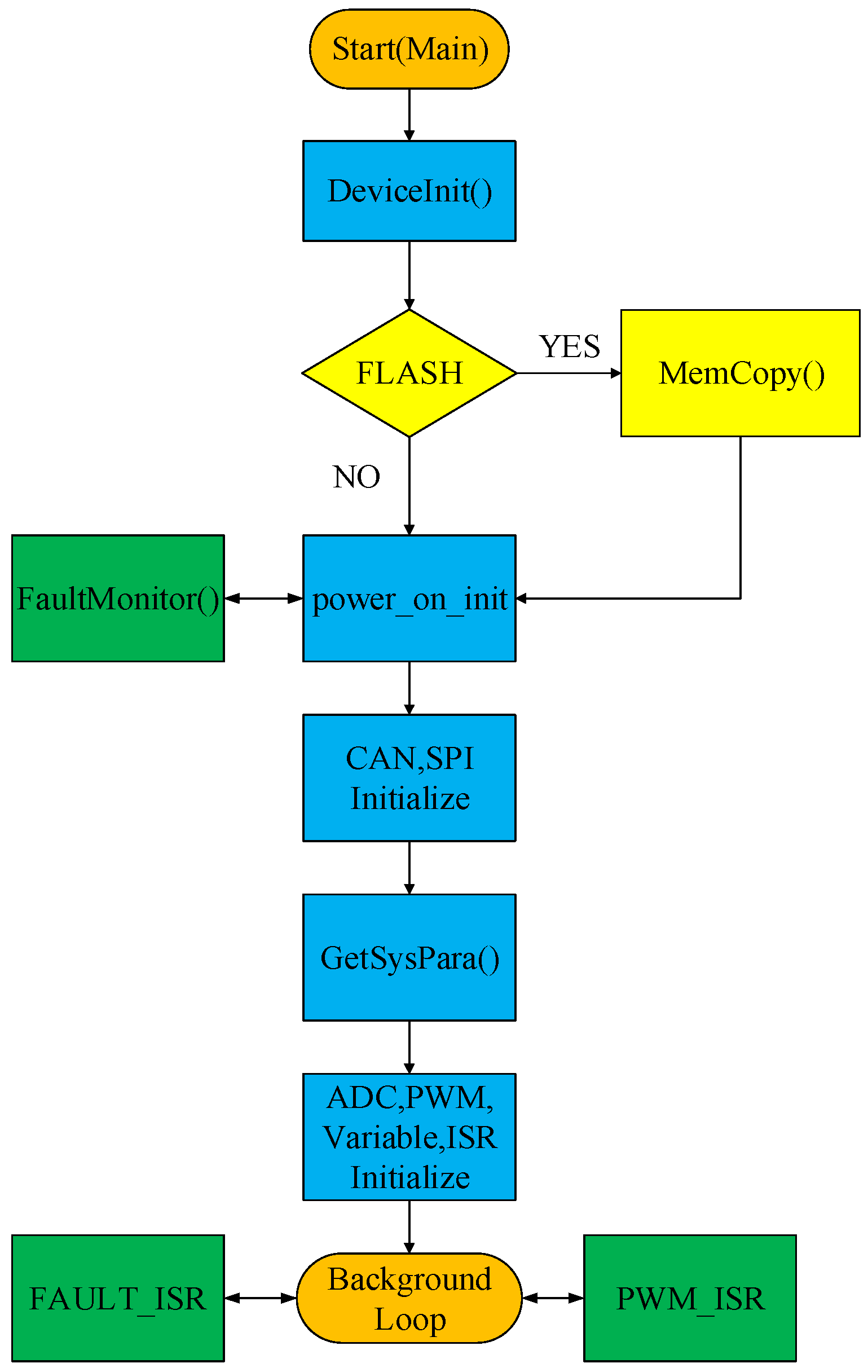
To carry out the model predictive control algorithm on the microcontroller, it is necessary to perform discretization and the variables in the program need to be normalized.

In the two-phase rotating coordinate frame, the estimated flux linkage of the current model can be represented as:

$${\psi }_{rd}\left[k\right]=K_1{\psi }_{rd}\left[k-1\right]+K_2{i}_{sd}pu$$

(52)

where:

$$K_1=\frac{T_r}{T_r+T_s},K_2=\frac{T_s}{T_r+T_s}$$

(53)

pu is short for per unit and is omitted in context below. In the two-phase stationary coordinate frame, the estimated flux linkage of the current model can be shown as:

$${\psi }_{s\alpha pu}^i\left[k\right]=K_3{\psi }_{r\alpha pu}^i\left[k\right]+K_4{i}_{s\alpha pu}\left[k\right]$$

(54)

$${\psi }_{s\beta pu}^i\left[k\right]=K_3{\psi }_{r\beta pu}^i\left[k\right]+K_4{i}_{s\beta pu}\left[k\right]$$

(55)

where:

$$K_3=\frac{L_m}{L_r},K_4=\frac{L_s{L}_r-L_m^2}{L_r{L}_m}$$

(56)

In the two-phase stationary coordinate frame, the electromotive force (EMF) estimation of the voltage model can be expressed as:

$$e_{s\alpha pu}\left[k\right]=u_{s\alpha pu}\left[k\right]-K_5{i}_{s\alpha }\left[k\right]-u_{com\alpha pu}\left[k\right]$$

(57)

$$e_{s\beta pu}\left[k\right]=u_{s\beta pu}\left[k\right]-K_5{i}_{s\beta }\left[k\right]-u_{com\beta pu}\left[k\right]$$

(58)

where:

$$K_5=\frac{I_b{R}_s}{V_b}$$

(59)

I_b is the base current, and V_b is the base phase voltage. In the two-phase stationary coordinate frame, the stator flux estimation can be represented as:

$${\psi }_{s\alpha pu}^v\left[k\right]={\psi }_{s\alpha pu}^v\left[k-1\right]+K_6\frac{\left(e_{s\alpha pu}\left[k\right]+e_{s\alpha pu}\left[k-1\right]\right) }{2}$$

(60)

$${\psi }_{s\beta pu}^v\left[k\right]={\psi }_{s\beta pu}^v\left[k-1\right]+K_6\frac{\left(e_{s\beta pu}\left[k\right]+e_{s\beta pu}\left[k-1\right]\right)}{2}$$

(61)

where:

$$K_6=\frac{V_b{T}_s}{L_m{I}_b}$$

(62)

In the two-phase stationary coordinate frame, the rotor flux estimation can be expressed as:

$${\psi }_{r\alpha pu}^v\left[k\right]=K_7{\psi }_{s\alpha pu}^v\left[k\right]-K_8{i}_{s\alpha pu}\left[k\right]$$

(63)

$${\psi }_{r\beta pu}^v\left[k\right]=K_7{\psi }_{s\beta pu}^v\left[k\right]-K_8{i}_{s\beta pu}\left[k\right]$$

(64)

where:

$$K_7=\frac{L_r}{L_m},K_8=\frac{L_s{L}_r-L_m^2}{L_m{L}_m}$$

(65)

The rotor flux linkage angle can be shown as:

$${\theta }_{rpu}\left[k\right]=\frac{1}{2\pi }{\tan }^{-1}\left(\frac{{\psi }_{r\beta pu}^v\left[k\right]}{{\psi }_{r\alpha pu}^v\left[k\right]}\right)$$

(66)

Equations (52)–(66) give the normalized formula used in the algorithm of the flux observer program.

The normalized speed calculation formula can be expressed as:

$${\omega }_{rpu}={\omega }_{epu}-K_9\frac{{\psi }_{r\alpha pu}{i}_{s\beta pu}-{\psi }_{r\beta pu}{i}_{s\alpha pu}}{{\psi }_{rpu}^2}$$

(67)

where:

$$K_9=\frac{1}{{\omega }_b{T}_r},{\omega }_b=2\pi f_b$$

(68)

${\omega }_b$ is the basic electrical rotating speed in rad/s. The discretized normalized flux linkage rotating speed can be expressed as:

$${\omega }_{epu}\left[k\right]=K_{10}\left({\theta }_{rpu}\left[k\right]-{\theta }_{rpu}\left[k-1\right]\right)$$

(69)

where:

$$K_{10}=\frac{1}{f_b{T}_{\mathrm{s}}}$$

(70)

Usually in the actual algorithm implementation, a first-order filter is used in the speed calculation, so it becomes:

$${\omega }_{epu}\left[k\right]=K_{11}{\omega }_{epu}\left[k-1\right]+K_{12}{\omega }_{epu}\left[k\right]$$

(71)

where:

$$K_{11}=\frac{{\tau }_{\mathrm{c}}}{{\tau }_{\mathrm{c}}+T_s},K_{12}=\frac{T_s}{{\tau }_{\mathrm{c}}+T_s},{\tau }_{\mathrm{c}}=\frac{1}{2\pi f_{\mathrm{c}}}$$

(72)

${\tau }_{\mathrm{c}}$ is the first-order filter time constant with $f_{\mathrm{c}}$ as the cutoff frequency.

After having the rotor flux value, the estimated speed can be obtained according to (67).

When the system is implemented, giving the parameters of K₁–K₁₂ and the motor parameters, then the flux linkage observer and speed estimation module can work as expected.

In the experimental model predictive control algorithm, there is often a one-step delay [27]. Having the estimated state variable at time k, the control vector U selected by the predictive cost function needs to wait for a sampling period before it can be applied to the motor control system. At that time, the state variable has become the value at [k + 1]. The current and flux sampled at [k + 1] use the measured voltage at k, and the torque and flux at [k + 2] are predicted. Therefore, some articles consider the system delay and use the state variable estimated at [k + 2] as feedback to perform the calculation of the cost function.

Considering the one-step delay, the cost function can be represented as:

$$\mathrm{J}={\left[I_{\alpha }-I_{\alpha }^p\left(k+2\right)\right]}^2+{\left[I_{\beta }-I_{\beta }^p\left(k+2\right)\right]}^2$$

(73)

3.5.2. Main Program

The FOC/MPC algorithm is implemented on a digital control unit and it is the key process of the motor controller for electric vehicles. Its control cycle is chosen the same as the PWM interrupt service cycle. Apart from the main FOC/MPC algorithm, the error diagnosis, field weakening control, overmodulation, current/voltage protection, communication with PC and VCU and some other practical contents are also considered when undertaking implementation [6].

The flow diagram of the main algorithm is shown in Figure 7. After the motor controller is powered up, the DeviceInit block works first, which initializes the system clock and GPIO. If the program is working on Flash, MemoryCopy block will copy the main interrupt service functions (ISRs) to RAM to save operation time. Then the CAN and SPI get initialized and motor parameters are retrieved from FRAM. After ADC and PWM are initialized, three functional tasks start operating in the background loop. Task A deals with the measurement and protection for voltage and current, monitor of the temperature, and it also collects some data for analysis online. Tasks B and C handle the communications with PC software and VCU. The data are coded by CAN protocol, which is common in electric vehicles. The driver instructions, such as starts and stops, speed acceleration or deceleration and changing gears, are all sent by CAN in these tasks. PWM_ISR contains the main algorithm for FOC and MPC, while FAULT_ISR works for fault diagnose [11].

The MPC program flow diagram in the PWM interrupt service function is shown in Figure 8. In general, the model predictive control algorithm first measures the voltage and current of the motor and then calculates the magnitude and angle of the rotor flux linkage. Next, it acquires the motor speed through the speed sensor and current model, or from the voltage model with the speed-sensorless algorithm. Then the predictive model predicts the stator current, torque and the magnitude of the flux linkage for the next step, and then uses the cost function to select the optimal control voltage. Finally, it generates the required PWM to drive the motor through the SVPWM algorithm.

4. Practical Problems

The motor control is implemented for real electric vehicles. Not only do the FOC and MPC algorithms need to be considered, but also some practical problems, such as initializing the excitation current [6], the current consistency of program and motor [11], field weakening control, over modulation, etc. Some of these issues are listed in this part.

4.1. Field-Weakening Control Strategy

The motor is supposed to reach rated power at the rated speed. A field-weakening control strategy is used for achieving higher speed with the capable power of the motor. The excitation current has to be decreased to weaken the flux linkage, and thus the motor can reach higher speed after the rated value. A variable $x_m$ is introduced here to represent the decreasing of the flux linkage.

$$x_m=f\left(v^{-1},v^{-2}\right)$$

(74)

where $v$ is the speed of the motor.

In this project, $x_m$ is chosen as:

$$x_m=\{\begin{array}{cc}0.83\ast v_m/v& if v\le 1.2\ast v_m\\ v_m^2/v^2& if v>1.2\ast v_m\end{array}$$

(75)

where $v_m$ is the rated speed, which equals 980 rpm (revolutions per minute).

4.2. Overmodulation

T₁ and T₂ are the durations of PWM obtained from the given U_ref ($U_{\alpha }, U_{\beta }$) according to SVPWM. The sum of T₁ and T₂ should be no more than the control period (unit 1). Therefore, improper U_ref could result in a wrong combination of T₁ and T₂, and then low power efficiency with current distortion may happen. An overmodulation strategy is used here to avoid this situation [28]. An easy but useful method is to decrease T₁ and T₂ by proportion and make the sum equal to 1. The logic diagram is shown in Figure 9.

4.3. PC Software

A specific PC software is designed for conducting the experiments for the motor controller. It combines functions such as downloading the motor parameters to the microprocessor, motor start, motor stop, monitor of program variables, etc. The communication protocol of CAN between PC software and MCU is also designed as needed.

5. Experimental Results and Discussion

The experiment setup is shown in Figure 10, with the current sensors, target induction motor, dynamometer, voltage source, oscilloscope, etc. The parameters of the target motor are listed in

Table 4. Motor parameters table.

Motor Parameters	Value	Unit
Rated power	100	kW
Rated voltage	350	V
Rated current	178	A
Rated speed	980	rpm
Number of pole pairs	3
Rr	0.014	Ω
Lr	10.5	mH
Rs	0.019	Ω
Ls	10.9	mH
Peak power	250	kW
Max torque	2400	Nm
Switching frequency	2~20	kHz

.

The experiment is carried out on an electric motor test-bench, which is supported by AVL. When the experiments are conducted for testing speed control, the towing motor will operate at a fixed torque. When the experiments are testing torque control, the towing motor will run at a fixed speed. By setting these up, the transient performance and steady-state performance can be tested as planned.

5.1. Field Weakening Control

Without flux weakening or using inappropriate $x_m$, the speed will get capped and cannot increase properly after reaching the rated value, as Figure 11 shows. Figure 12 shows the proper speed performance by applying $x_m$ as Equation (75). Figure 11 and Figure 12 are both obtained from the CAN signal analysis tool PcanExplorer. There is a bias of 12,735 in Y-axis for current variables and the values are 10 times of the real values for I_d and I_q, respectively. The speed value in the figure equals its real value. The different performance of speed in Figure 11 and Figure 12 verifies the significance of the field-weakening control strategy. A good strategy can lead to a better speed range in motor control for electric vehicles.

5.2. Overmodulation

Figure 13 shows the effect of using an overmodulation strategy. All three phase voltages can reach a higher level responding to an increase in I_q through overmodulation and the torque can achieve a higher value in response. For deeper voltage utilization, the overmodulation can be designed in three phases based on the magnitude of the reference voltage. If the overmodulation strategy does not apply to the motor control system, the torque will become unstable when higher I_q is needed in overload situations.

5.3. Torque Peformances

When an acceleration instruction is given by the driver, it will be converted to an $I_q$ value for the motor control and then executed to acquire the demanded torque. The motor controller will deal with the instruction and increases the speed of the vehicle as a response. As for the experiments in the laboratory, the motor controller is connected to a PC simulator and receives instructions from the specific software. The load motor can be set at a fixed speed and then $I_q$ is changed step by step to acquire the torque performance of the target motor.

The FOC and MPC methods are both carried out in experiments. Figure 14 shows the responses of torque with different values of $I_q$ in the FOC method. The torque ripples with the FOC method are shown in Figure 15. For the MPC method, Figure 16 and Figure 17 present the torque responses and torque ripples. In these experiments, the load motor is set at a fixed 980 rpm and thus increasing the I_q of the tested motor will not accelerate the motor speed. The sampling frequency is set to 4 K for the FOC method and 16 K for the MPC method. Torque is tested in a large working span, which is from 0 Nm to about 1800 Nm. The excitation current I_d is given first to establish the flux. I_q is given after the flux has been established and then increases step by step. Using this pre-excitation strategy can effectively reduce the large starting current. Figure 14, Figure 15, Figure 16 and Figure 17 show that, with either the FOC or MPC method, the torque is very stable with a ripple of under 3% throughout the working area, which is normally considered as a good performance for electric vehicles. The transient responses are both satisfactory as well. The ripple with the MPC method is slightly better than with the FOC method, as shown by the figures.

With these experiments, it seems that MPC for a motor control system is not significantly better than the FOC method. It has to be mentioned that an FOC with such a good performance comes from tuning the PID parameters with a lot of time while MPC does not need so much time on tuning. In this paper, there are 12 voltage vectors chosen for MPC optimization, which leads to a good performance but high time consumption. To acquire better performance of the MPC, the control frequency can be set higher. However, it will make the IGBT switching frequency become higher [29]. For a longer serving life of IGBT, a compromise has to be made about the control frequency. The experimental results show that MPC is an alternative control strategy to FOC for the motor control systems of electric vehicles and MPC has great potential abilities for further study.

6. Conclusions

This paper introduces the implementation of a motor control for electric vehicles based on the FOC and MPC methods. It discusses the model of motor, hardware of the system, flux estimation, speed estimation, discretization, normalization, etc. The implementation algorithms are explained in detail, which could be helpful for motor controller design. For electric vehicles, motor control should not only be studied within the rated range, so that some practical algorithms such as field-weakening control and overmodulation considering variations of the load that exist in electric vehicles are also discussed here. The performances of the FOC and MPC methods are compared with experiments. The experiments are conducted with a 100 kW induction motor. The torque responses are fast and stable with both of the methods, which are satisfactory. The 12 basic vectors FOC has a torque ripple under ±3% within rated power, which is great among the currently used vector controls of induction motors. This motor controller is flexible to match different types of induction motors and thus it can be widely used for electric vehicles.

References

1. Xu, W.; Zhu, J.; Guo, Y.; Wang, S.; Wang, Y.; Shi, Z. Survey on electrical machines in electrical vehicles. In Proceedings of the 2009 International Conference on Applied Superconductivity and Electromagnetic Devices, ASEMD 2009, Chengdu, China, 25–27 September 2009; pp. 167–170. [Google Scholar]
2. Lei, G.; Wang, T.S.; Guo, Y.G.; Zhu, J.G.; Wang, S.H. System-Level Design Optimization Methods for Electrical Drive Systems: Deterministic Approach. IEEE Trans. Ind. Electron. 2014, 61, 6591–6602. [Google Scholar] [CrossRef]
3. Lei, G.; Wang, T.S.; Zhu, J.G.; Guo, Y.G.; Wang, S.H. System-Level Design Optimization Method for Electrical Drive Systems-Robust Approach. IEEE Trans. Ind. Electron. 2015, 62, 4702–4713. [Google Scholar] [CrossRef]
4. Chan, C.C. The state of the art of electric and hybrid vehicles. Proc. IEEE 2002, 90, 247–275. [Google Scholar] [CrossRef] [Green Version]
5. Berrezzek, F.; Bensaker, B. Flatness based nonlinear sensorless control of induction motor systems. Int. J. Power Electron. Drive Syst. 2016, 7, 265. [Google Scholar]
6. Men, X.; Guo, Y.; Wu, G.; Shi, C.; Zhu, J. Implementation of a motor control system for electric bus based on DSP. In Proceedings of the 2017 20th International Conference on Electrical Machines and Systems (ICEMS), Sydney, Australia, 11–14 August 2017; pp. 1–6. [Google Scholar]
7. Dannehl, J.; Fuchs, F.W. Flatness-based control of an induction machine fed via voltage source inverter-concept, control design and performance analysis. In Proceedings of the IECON 2006-32nd Annual Conference on IEEE Industrial Electronics, Paris, France, 6–10 November 2006; pp. 5125–5130. [Google Scholar]
8. Fan, L.; Zhang, L. An improved vector control of an induction motor based on flatness. Procedia Eng. 2011, 15, 624–628. [Google Scholar] [CrossRef]
9. Casadei, D.; Profumo, F.; Serra, G.; Tani, A. FOC and DTC: Two viable schemes for induction motors torque control. IEEE Trans. Power Electron. 2002, 17, 779–787. [Google Scholar] [CrossRef] [Green Version]
10. Bose, B.K.; Simoes, M.G.; Crecelius, D.R.; Rajashekara, K.; Martin, R. Speed sensorless hybrid vector controlled induction motor drive. In Proceedings of the Conference Record of the 1995 IEEE Industry Applications Conference Thirtieth IAS Annual Meeting, Orlando, FL, USA, 8–12 October 1995; pp. 137–143. [Google Scholar]
11. Men, X.; Wu, G.; Guo, Y.; Zhu, Z.; Gao, J. Development of an Advanced Motor Control System for Electric Vehicles; SAE Technical Papers; SAE International: Detroit, MI, USA, 2019. [Google Scholar]
12. Vazquez, S.; Leon, J.; Franquelo, L.; Rodriguez, J.; Young, H.A.; Marquez, A.; Zanchetta, P. Model predictive control: A review of its applications in power electronics. IEEE Ind. Electron. Mag. 2014, 8, 16–31. [Google Scholar] [CrossRef]
13. Rodriguez, J.; Kazmierkowski, M.P.; Espinoza, J.R.; Zanchetta, P.; Abu-Rub, H.; Young, H.A.; Rojas, C.A. State of the art of finite control set model predictive control in power electronics. IEEE Trans. Ind. Inform. 2013, 9, 1003–1016. [Google Scholar] [CrossRef]
14. Zhang, Y.; Yang, H. Generalized two-vector-based model-predictive torque control of induction motor drives. IEEE Trans. Power Electron. 2015, 30, 3818–3829. [Google Scholar] [CrossRef]
15. Zhang, Y.; Yang, H.; Li, Z. A simple SVM-based deadbeat direct torque control of induction motor drives. In Proceedings of the 2013 International Conference on Electrical Machines and Systems (ICEMS), Busan, Korea, 26–29 October 2013; pp. 2201–2206. [Google Scholar]
16. Rodriguez, J.; Cortes, P. Predictive Control of Power Converters and Electrical Drives; John Wiley & Sons: New York, NY, USA, 2012; Volume 40. [Google Scholar]
17. Miranda, H.; Cortés, P.; Yuz, J.I.; Rodríguez, J. Predictive torque control of induction machines based on state-space models. IEEE Trans. Ind. Electron. 2009, 56, 1916–1924. [Google Scholar] [CrossRef]
18. Chapra, S.C.; Canale, R.P. Numerical Methods for Engineers; McGraw-Hill Higher Education: Boston, MA, USA, 2010. [Google Scholar]
19. Zhang, Y.; Yang, H. Two-vector-based model predictive torque control without weighting factors for induction motor drives. IEEE Trans. Power Electron. 2016, 31, 1381–1390. [Google Scholar] [CrossRef]
20. Cortés, P.; Kouro, S.; La Rocca, B.; Vargas, R.; Rodríguez, J.; León, J.I.; Vazquez, S.; Franquelo, L.G. Guidelines for weighting factors design in model predictive control of power converters and drives. In Proceedings of the 2009 IEEE International Conference on Industrial Technology, Churchill, Australia, 10–13 February 2009; pp. 1–7. [Google Scholar]
21. Akin, B.; Bhardwaj, M. Sensored Field Oriented Control of 3-Phase Induction Motors; Texas Instrument Guide; Texas Instruments Incorporated: Dallas, TX, USA, 2013; p. 2019. [Google Scholar]
22. Mariethoz, S.; Domahidi, A.; Morari, M. High-bandwidth explicit model predictive control of electrical drives. IEEE Trans. Ind. Appl. 2012, 48, 1980–1992. [Google Scholar] [CrossRef]
23. Geyer, T.; Papafotiou, G.; Morari, M. Model predictive direct torque control—Part I: Concept, algorithm, and analysis. IEEE Trans. Ind. Electron. 2009, 56, 1894–1905. [Google Scholar] [CrossRef]
24. Zhang, Y.; Zhao, Z. Speed sensorless control for three-level inverter-fed induction motors using an extended Luenberger observer. In Proceedings of the 2008 IEEE Vehicle Power and Propulsion Conference, Harbin, China, 3–5 September 2008; IEEE: Piscataway, NJ, USA, 2008; pp. 1–5. [Google Scholar]
25. Zhang, Y.; Zhu, J. An improved direct torque control for three-level inverter-fed induction motor sensorless drive. IEEE Trans. Power Electron. 2012, 27, 1502–1513. [Google Scholar] [CrossRef]
26. Zhang, Y.; Yang, H.; Xia, B. Model-predictive control of induction motor drives: Torque control versus flux control. IEEE Trans. Ind. Appl. 2016, 52, 4050–4060. [Google Scholar] [CrossRef]
27. Seman, S.; Niiranen, J.; Arkkio, A. Ride-through analysis of doubly fed induction wind-power generator under unsymmetrical network disturbance. IEEE Trans. Power Syst. 2006, 21, 1782. [Google Scholar] [CrossRef]
28. Lee, D.; Lee, G. A novel overmodulation technique for space-vector PWM inverters. IEEE Trans. Power Electron. 1998, 13, 1144–1151. [Google Scholar]
29. Zhang, Y.; Xia, B.; Yang, H. Performance evaluation of an improved model predictive control with field oriented control as a benchmark. IET Electr. Power Appl. 2017, 11, 677–687. [Google Scholar] [CrossRef]
Figure 1. Diagram of motor control.
Energies 15 04833 g001
Figure 2. Scheme of FOC based on a digital controller.
Energies 15 04833 g002
Figure 3. SVPWM scheme: U1–U6 are the basic vectors, U0 and U7 are the zero vectors, and Ts is the control period.
Energies 15 04833 g003
Figure 4. Scheme of MPC based on a digital controller.
Energies 15 04833 g004
Figure 5. Basic space vectors scheme. Each voltage vector projects to a specific combination of U α and U β . Twelve combinations and two zero vectors build up the basic voltage control set.
Energies 15 04833 g005
Figure 6. Speed calculation program flow diagram.
Energies 15 04833 g006
Figure 7. Main program flow diagram.
Energies 15 04833 g007
Figure 8. MPC program flow diagram.
Energies 15 04833 g008
Figure 9. Overmodulation logic diagram.
Energies 15 04833 g009
Figure 10. Experiment setup.
Energies 15 04833 g010
Figure 11. Speed and Id responses versus changing Iq when x m is not appropriate.
Energies 15 04833 g011
Figure 12. Speed and Id responses versus changing Iq when x m is appropriate.
Energies 15 04833 g012
Figure 13. Voltage and torque responses versus changing Iq. Red curve represents the system running in overmodulation mode and blue curve in no overmodulation mode.
Energies 15 04833 g013
Figure 14. Torque responses versus changing Iq with the FOC method.
Energies 15 04833 g014
Figure 15. Torque ripples with the FOC method.
Energies 15 04833 g015
Figure 16. Torque responses versus changing Iq with the MPC method.
Energies 15 04833 g016
Figure 17. Torque ripples with the MPC method.
Energies 15 04833 g017