Abstract
The estimation of non-stationary random medium parameters of petrophysical parameters is the key to the application of random medium theory in fine seismic exploration. We proposed a method for estimating non-stationary random medium parameters of petrophysical parameters using seismic data. Based on the linear petrophysical model, the relationship between seismic data and porosity, clay volume, and water saturation in the random medium was described, and the principle and method of estimating the autocorrelation parameters of the petrophysical parameter random medium were introduced in this study. Subsequently, the specific steps of applying the power spectrum method, for parameter estimation in non-stationary random media with petrophysical parameters, were explained. The feasibility and correctness of the method were verified through the estimation test of the two-dimensional theoretical model. Eventually, the estimation test of non-stationary random medium parameters of petrophysical parameters was carried out by field seismic data, and the results indicated that the non-stationary random medium parameters can better portray the information of subsurface medium petrophysical parameters. The method can provide a reference for the construction of a priori information on petrophysical parameters, and it can also provide a theoretical basis for the in-depth application of random medium theory to practical data.
1. Introduction
When studying reservoir structure or sedimentology, the heterogeneity of underground media can be categorized into two scales: large and small. Large-scale heterogeneity describes the background trend and slowly variable characteristics of the subsurface media, and small-scale heterogeneity describes the small-scale perturbation of the subsurface media attached to the background trend [1]. Because of the random perturbation characteristics in small-scale heterogeneity, conventional deterministic modeling methods cannot provide a complete description of it. Ikelle [2] regarded the subsurface media parameters as random variables and characterized the heterogeneity in the subsurface media modeling via the random medium statistical principles. However, this method cannot determine the statistics of parameters in the subsurface medium, due to its limitation in the application and discussion of the theoretical model, which increases the application difficulties in field seismic exploration. Reflected seismic data inherit the heterogeneity of this random distribution of the subsurface medium; thus, it is possible to estimate the random medium parameters from reflected seismic data [3,4]. The stratigraphic interface in sedimentary basins is usually continuous with strong reflection waves, and for small-scale media in the strata, seismic waves behave discontinuously with weak reflection waves [5]. It is crucial to quantify the relationship between small-scale heterogeneity and discontinuous reflected waves, as well as to characterize the underground small-scale heterogeneity. Gibson [6] first approximated the horizontal autocorrelation function of post-stack seismic data to the horizontal heterogeneity in the subsurface media. Poppeliers [7] inverted the vertical autocorrelation function and its characteristic parameters of post-stack seismic data, via the deconvolution method, to characterize the vertical heterogeneity of the subsurface media. Although the above-mentioned two methods have been used in seismic interpretations [4], they are both estimated from the horizontal and vertical directions, which are both estimated in one-dimensional cases [8,9,10]. There is still a considerable difference in the characterization of heterogeneity for the two-dimensional and three-dimensional cases.
To accommodate the modern seismic data, Irving [11] and Scholer [12] further established the relationship equation between the two-dimensional subsurface media and the post-stack seismic data, and they estimated both horizontal and vertical autocorrelation functions from the post-stack seismic data by using the Monte Carlo inversion method. However, the estimated autocorrelation function of this method is still one-dimensional and is only applicable in the case of simple underground heterogeneity. The estimated horizontal and vertical autocorrelation functions are always subject to large errors when the underground structure is complex, the dip angle of the strata varies greatly, and the disturbance direction of the subsurface medium varies with the horizontal and vertical angles. Gu [5], in his Ph. D. thesis [13], proposed the method for estimating stationary and non-stationary random medium parameters, from two-dimensional post-stack seismic data, based on the power spectrum method. Based on the relationship between the post-stack seismic data and the wave impedance random medium model, they derived the estimation method of wave impedance random medium parameters, which innovatively realized the simultaneous estimation of two-dimensional autocorrelation length and autocorrelation angle. The random medium theory has also been used to estimate different parameter information, such as the prediction of structure-specific parameter information by random medium models [14], the estimation of fracture and anisotropic fracture parameters in subsurface media [15,16,17], and the description of the crustal structure by estimating two-dimensional horizontal autocorrelation length information [18]. Yang [19,20] applied the autocorrelation length and autocorrelation angle to the simulation process in field data inversion to assess the uncertainty of the inversion. Although the autocorrelation length and angle are estimated from well data and geological understanding, which is a large-scale mean value, the estimates do not describe the small-scale heterogeneity in the subsurface media. Fan [21] estimated the horizontal autocorrelation length of deep seismic reflection profiles based on the random model, which could not fully describe the heterogeneity of the subsurface media. Wang [22] applied the elastic random medium parameters to the initial model construction of real data to describe the heterogeneity of the subsurface medium. When estimating the random medium parameters, the above scholars mostly considered the estimation of the elastic random medium parameters and rarely considered the estimation of the petrophysical non-stationary random medium parameters. At present, the modeling and application of the random medium theory, in the estimation of the actual petrophysical parameters, need to be improved.
To solve the before-mentioned problem, we derived the power spectrum relationship between the random medium model of porosity, clay volume, and water saturation and the seismic data, based on a linear petrophysical model, and proposed a non-stationary random medium parameter estimation method for the petrophysical parameters. The method can simultaneously estimate nine characteristic parameters of porosity, water saturation, and clay volume in horizontal and vertical autocorrelation lengths and angles. Finally, the proposed estimation method was tested and analyzed using the model data, and it was applied to the field seismic data.
2. Methods
2.1. Mathematical Characterization of Random Medium
The theory of random media was discovered by the Polish scholar Litwiniszyn [23], in 1956, during his study on the movement of rock masses. He believed that the motion of rock masses is controlled by a large number of known and unknown factors, and he solved their motion processes by considering them as random media. The random medium model can characterize the random variation in the rock’s physical properties space. In studying the heterogeneity of the subsurface medium, the subsurface medium is usually divided into different scales for mathematical characterization. The large-scale heterogeneity characterizes the average characteristics of the subsurface media. It is described by the mean value of the first-order statistics, which can be expressed by the traditional deterministic method through observation data. The small-scale heterogeneity characterizes the random perturbation properties of the subsurface medium; that is, it is described by the second-order statistical variance and autocorrelation functions, which can be mathematically characterized by a random medium model based on random medium theory. The random medium model is defined as follows:
where represents the standard deviation of the random media model. means that the mean is zero, the standard deviation is one, and the spatial perturbation characteristics obey the random disturbance model of the two-dimensional autocorrelation function .
When characterizing the small-scale heterogeneity of the subsurface medium by the random medium model, the scale and direction of the random perturbation are mainly controlled by the autocorrelation function, and the range of the value of the random perturbation is controlled by the standard deviation. The commonly used analytical forms of the autocorrelation function are Gaussian elliptic autocorrelation function, exponential elliptic autocorrelation function, mixed elliptic autocorrelation function, Von Kármán autocorrelation function, and fractal autocorrelation function. Xi and Yao [24] analyzed and summarized the Gaussian elliptic autocorrelation function and exponential elliptic autocorrelation function, and they proposed a mixed elliptic autocorrelation function that combines the advantages of both and can be adjusted dynamically.
where a indicates the horizontal autocorrelation length, b stands for the vertical autocorrelation length, denotes the autocorrelation angle, and signifies the roughness factor. When , the autocorrelation function is Gaussian, and when , the autocorrelation function is exponential, when changes from zero to one, the autocorrelation function gradually changes and transitions between Gaussian and exponential. By varying the value of the mixed autocorrelation function roughness factor , it is feasible to dynamically characterize the type of heterogeneity of the subsurface media.
2.2. Estimation Principles of Stationary Random Medium Parameters for Petrophysical Parameters
The first step of studying the estimation method of random medium parameters is to begin with a random medium model with different elastic parameters. The p-wave velocity, s-wave velocity, and density models of random media can be defined as follows [2,13,25,26]:
where , and represent the mean values of p-wave velocity, s-wave velocity, and density, respectively. The mean value characterizes the background trend; that is, the low-frequency component. , and are the relative disturbances added to the background trend: namely, the high-frequency component.
The next step is to begin with a random medium model with different petrophysical parameters. The random medium porosity , clay volume , and water saturation models can be defined as follows:
where , and stand for the mean values of porosity, clay volume, and water saturation, respectively. , and are the relative perturbation added to the background trend.
In field data processing, the relationship between elastic parameters and petrophysical parameters is chiefly nonlinear, which can be obtained by curve fitting, such as Gaussian fitting and polynomial fitting. It can be regarded as a linear relationship under the condition of error tolerance [27,28,29].
The coefficient and the constant term in Equation (6) can be obtained by multiple regression fitting using well data.
According to the elastic impedance equation, published by Connolly [30] on The Leading Edge in 1999, the reflection coefficient can be expressed as follows:
where denotes the incidence angle, .
Inspired by Gu [5,13], who established the relationship between post-stack seismic data and the wave impedance random medium model, we further established the relationship between the partial angle stacked seismic data and porosity, clay volume, and water saturation random medium model.
Thus, the power spectrum of porosity , clay volume , and water saturation is expressed as follows:
where is Hadamard product, symbolizes the Fourier transform results of at different incidence angles, respectively. signify the coefficients at different incidence angles, and indicates the Fourier transformed data of B at different incidence angles. and B are detailed in Appendix A.
Therefore, according to the Wiener–Khinchin theorem, the autocorrelation function of porosity , clay volume , and water saturation can be procured by performing the Fourier inverse transformation on the power spectrum data.
The method further derives the autocorrelation functions of porosity, clay volume, and water saturation, based on the relationship between elastic and petrophysical parameters, using partial angle stacked data from the pre-stack seismic. Based on the autocorrelation functions of the three petrophysical parameters, the random medium parameters (horizontal autocorrelation length, vertical autocorrelation length, and autocorrelation angle), corresponding to porosity, clay volume, and water saturation, are obtained. Appendix A includes the detailed formula derivations process of Equation (6) to Equation (9).
2.3. Estimation Process of Non-Stationary Random Medium Parameters
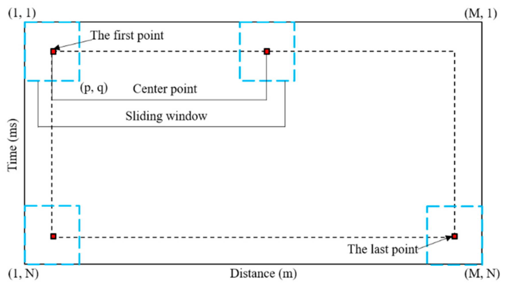
Our proposed method for estimating parameters of petrophysical parameter non-stationary random medium regards the whole of the estimated data as a non-stationary case and assumes that the data within a small local window is a stationary case. The window is first set up and the random medium autocorrelation parameters are estimated at the center position of the window. When all the points are iterated, the estimation of the non-stationary random medium parameters can be completed.
The process of estimating the parameters of a petrophysical parameter non-stationary random medium is as follows:
① The pre-stack seismic data are divided into three different angle ranges for partial stacking at different angles to obtain partially stacked seismic data at different center angles.
② Estimation of seismic wavelets, for cases with different central angles, based on partially stacked seismic data at different angles, respectively.
③ Set the size of the sliding window and the sliding interval at the same time, select the starting position of the estimated data, and perform simultaneous estimation of the stacked seismic data for different angle sections.
④ The sliding window position is unchanged for the first estimation and changes according to the sliding interval when the number of estimates is equal to, or larger than, two. Calculate the power spectrum of half the wavelet partial derivative and the power spectrum of the seismic data , and calculate the total power spectrum of the elastic impedance random medium .
⑤ Calculate the random medium power spectrum of porosity, clay volume, and water saturation, according to the Equation (8). After the inverse Fourier transform, the autocorrelation functions , , and of porosity, clay volume, and water saturation are calculated.
⑥ Binarize the autocorrelation function by setting the points of the autocorrelation functions , , and to 1, respectively. Set the points of , , and to 0, so the points assigning the autocorrelation function to 1 form an ellipse.
⑦ In the assigned autocorrelation function, extract the boundaries of the ellipse, assign X and Y variables, and find the center position of the ellipse. Define that the counterclockwise direction with the horizontal axis is negative, and calculate the normalized second-order center distance of the area.
⑧ The semi-major axis of the calculated ellipse is the horizontal autocorrelation length, the semi-minor axis is the vertical autocorrelation length, and the angle with the positive direction of the horizontal axis is the autocorrelation angle. The calculated autocorrelation parameters are the autocorrelation parameters at the center of the sliding window.
⑨ Repeat steps ④ to ⑧ until all points are iterated and stop iterating. Then, the random medium autocorrelation parameters of the porosity, clay volume, and water saturation can be obtained.
Figure 1 shows the parameter estimation strategy of a non-stationary random medium.

Figure 1.
Parameter estimation strategy of a non-stationary random medium.
3. Numerical Examples
3.1. Autocorrelation Parameter Estimation of Four-Layer Model
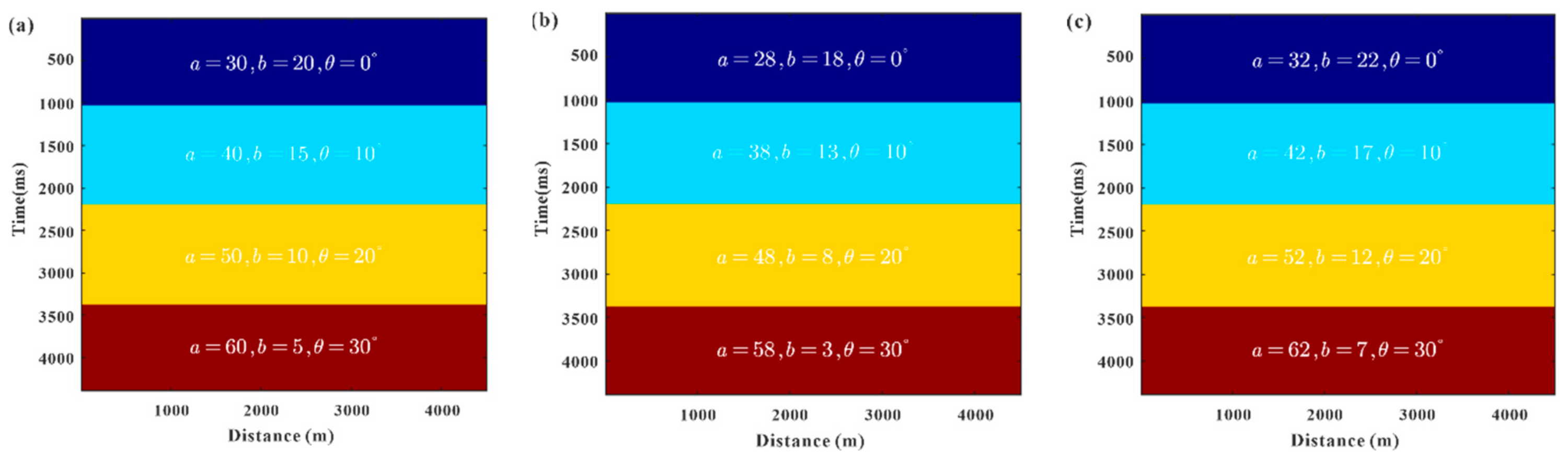
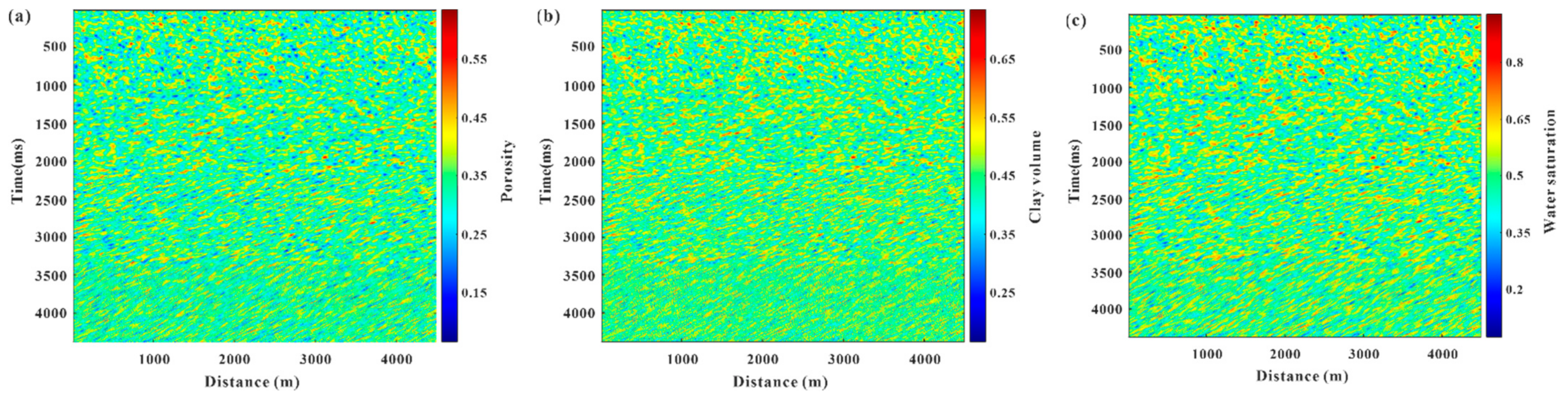
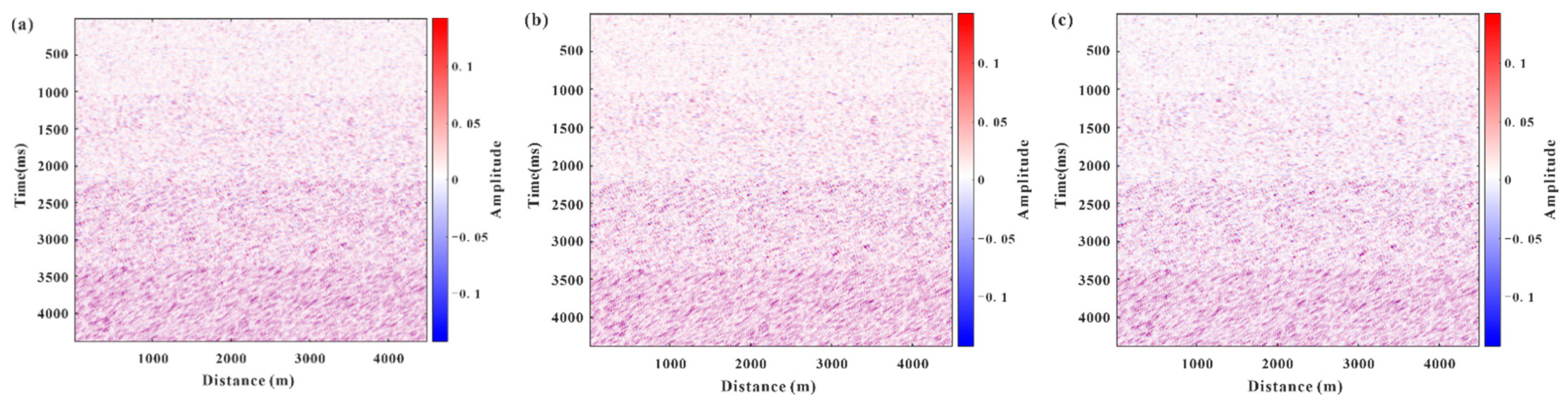
We set the random medium parameters of porosity, clay volume, and water saturation. The specific values are shown in Figure 2. We modeled the porosity, clay volume, and water saturation according to the set autocorrelation parameters. The grid size was Nx = Nt = 4500, the grid interval was dx = 1 m, dt = 1 ms, the mean porosity was 0.4 with a standard deviation of 0.05, the mean clay volume was 0.4 with a standard deviation of 0.08, and the mean water saturation was 0.5 with a standard deviation of 0.08. The mean p-wave velocity was 2121 m/s with a standard deviation of 588 m/s, the mean s-wave velocity was 774 m/s with a standard deviation of 454 m/s, and the mean density was 2113 g/cm3 with a standard deviation of 139 g/cm3. Figure 3a–c show the porosity, clay volume, and water saturation models, respectively. P-wave velocity, s-wave velocity, and density were simulated based on the mean and standard deviation of elastic parameters, and linear petrophysical model relationships were solved based on elastic and petrophysical variables. The Ricker wavelet was set with a dominant frequency of 35 Hz. The synthetic seismic data is generated by the Robinson convolution model, using reflection coefficients and Ricker wavelet. Figure 4a–c are synthetic seismic records with center angles of 7°, 18°, and 26°, respectively. Before estimation, we need to determine the range of values for the higher value of the autocorrelation length of the target layer, with a sliding window of roughly five times the size of the autocorrelation length (Gu, 2013, 2014) [5,13]. We set the sliding window size to 300 × 300 and combined the synthetic seismic data from different angles to estimate the autocorrelation parameters of three petrophysical parameters.
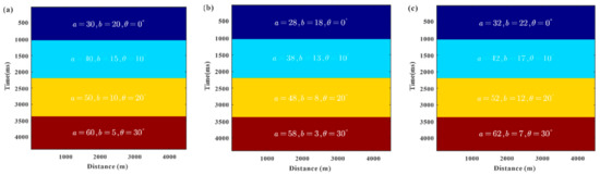
Figure 2.
Autocorrelation parameters: (a) porosity, (b) clay volume, (c) water saturation.
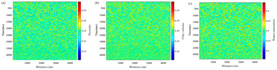
Figure 3.
Petrophysical parameter model: (a) porosity, (b) clay volume, (c) water saturation.
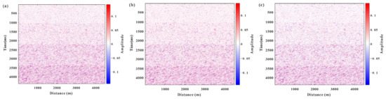
Figure 4.
Synthetic seismic data from different center angles: (a) 7°, (b) 18°, (c) 26°.
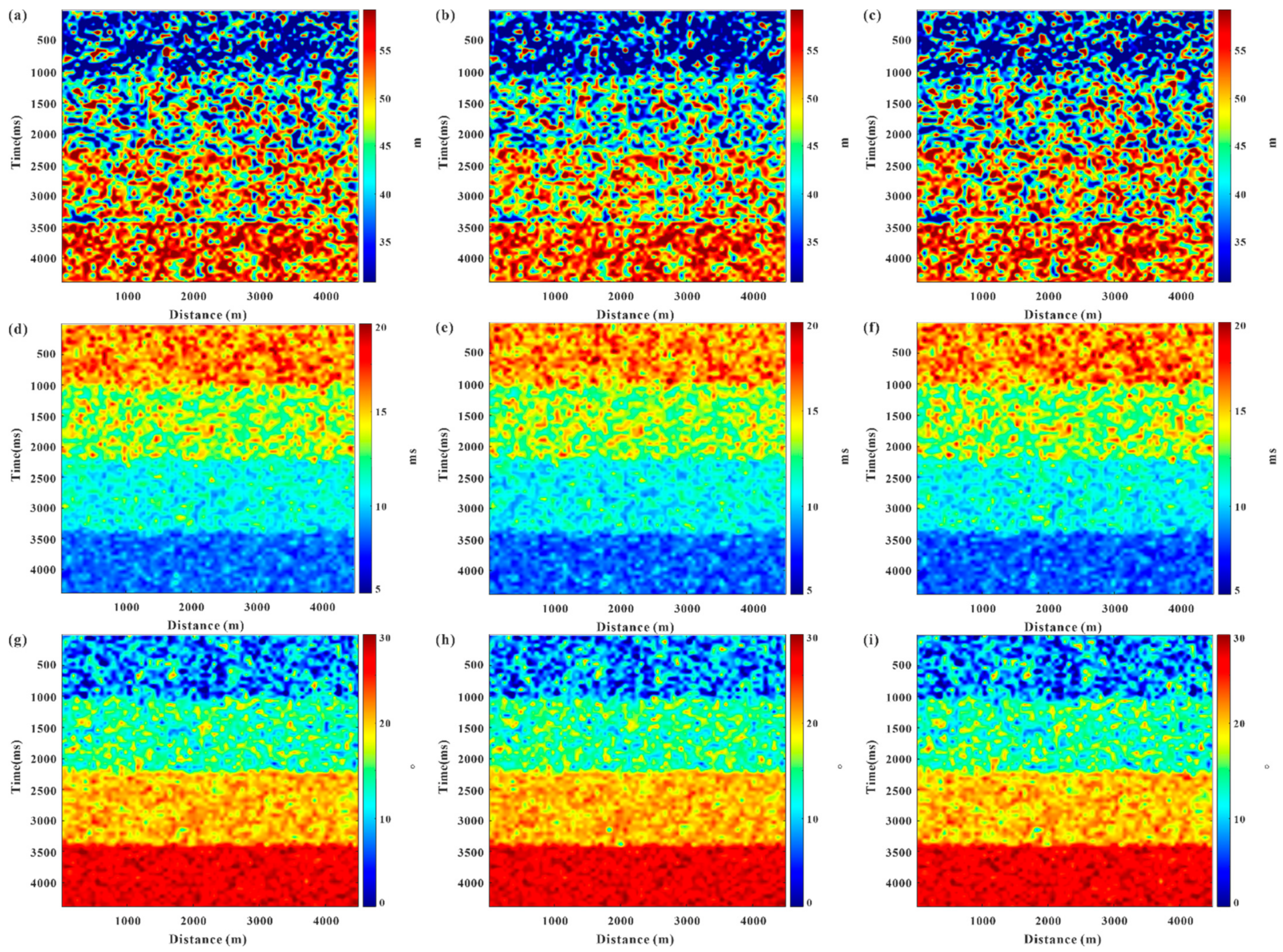
The parameter estimation results are shown in Figure 5. The estimation results are the values of the autocorrelation length and autocorrelation angle of different petrophysical parameters at each point. Figure 5a,d,g, respectively, represent the horizontal autocorrelation length, vertical autocorrelation length, and autocorrelation angle of porosity. Figure 5b,e,h represent the horizontal autocorrelation length, vertical autocorrelation length, and autocorrelation angle of clay volume, respectively. Figure 5c,f,I represent the horizontal autocorrelation length, vertical autocorrelation length, and autocorrelation angle of water saturation, respectively. Although the estimation result shown in the figure cannot completely correspond to the autocorrelation length and autocorrelation angle of the actual model, the error is about 20%. However, the four layers with distinct differences can still be clearly identified, and the estimated result is closer to the theoretical model.
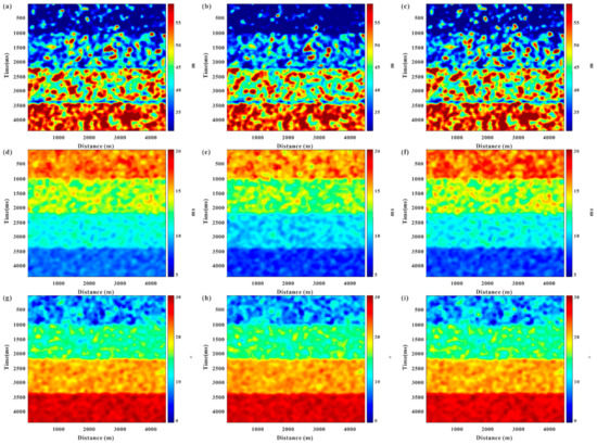
Figure 5.
Estimation results of autocorrelation parameters of porosity, clay volume, and water saturation: (a–c) are the horizontal autocorrelation length of porosity, clay volume, and water saturation, respectively. (d–f) are the vertical autocorrelation length of porosity, clay volume, and water saturation, respectively. (g–i) are the autocorrelation angle of porosity, clay volume, and water saturation, respectively.
In order to test the effect of the sliding window size on the estimation results in this method, we change the sliding window size for testing. When the sliding window size is set to 100 × 100, the size of the sliding window is less than five times the maximum autocorrelation length. A sliding window size of 100 × 100 is used as an example for testing. Figure 6 shows the parameter estimation results. It can be seen from the results that, when the sliding window is small, the vertical autocorrelation length, as well as the autocorrelation angle, can also identify the different four layers more clearly. However, the vertical autocorrelation lengths and autocorrelation angles within each layer vary, rapidly, both horizontally and vertically. The overall horizontal autocorrelation length varies rapidly and is too noisy to clearly identify the four layers. Tests show that the estimation results with a sliding window set to 100 × 100 are worse than those with a sliding window of 300 × 300. Therefore, before parameter estimation, the reasonable sliding window size should be determined first.
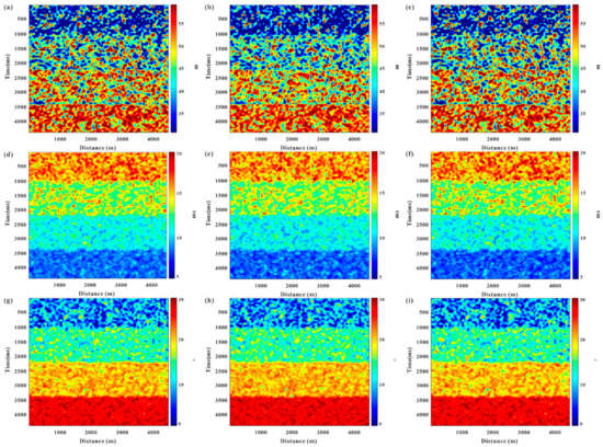
Figure 6.
Estimation results of autocorrelation parameters of porosity, clay volume, and water saturation: (a–c) are the horizontal autocorrelation length of porosity, clay volume, and water saturation, respectively. (d–f) are the vertical autocorrelation length of porosity, clay volume, and water saturation, respectively. (g–i) are the autocorrelation angles of porosity, clay volume, and water saturation, respectively.
The robustness of the method in this paper is verified by the noise test under different signal-to-noise ratios. The test result with a signal-to-noise ratio of 3 is taken, as an example, to show the estimation effect of the method in the case of seismic data with noise. We added Gaussian white noise to the seismic data and used the noise-containing seismic data with a signal-to-noise ratio of three (Figure 7) for the random medium parameter estimation of the petrophysical parameters. The sliding window is set to 300 × 300. Figure 8 exhibits the parameter estimation results, in which the estimation errors of horizontal autocorrelation length and autocorrelation angle of petrophysical parameters are smaller than those of vertical autocorrelation length, and the average error of parameter estimation can be controlled within 25%. The estimation result can also identify the four layers with clear differences and has better noise immunity.
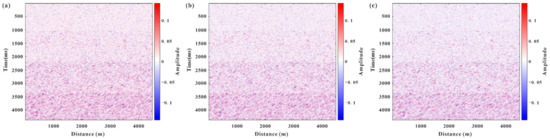
Figure 7.
Noise-containing synthetic seismic data from different center angles: (a) 7°, (b) 18°, (c) 26°.
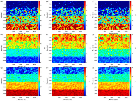
Figure 8.
Estimation results of autocorrelation parameters of porosity, clay volume, and water saturation: (a–c) are the horizontal autocorrelation length of porosity, clay volume, and water saturation, respectively. (d–f) are the vertical autocorrelation length of porosity, clay volume, and water saturation, respectively. (g–i) are the autocorrelation angle of porosity, clay volume, and water saturation, respectively.
3.2. Autocorrelation Parameter Estimation of Marmousi2 Model
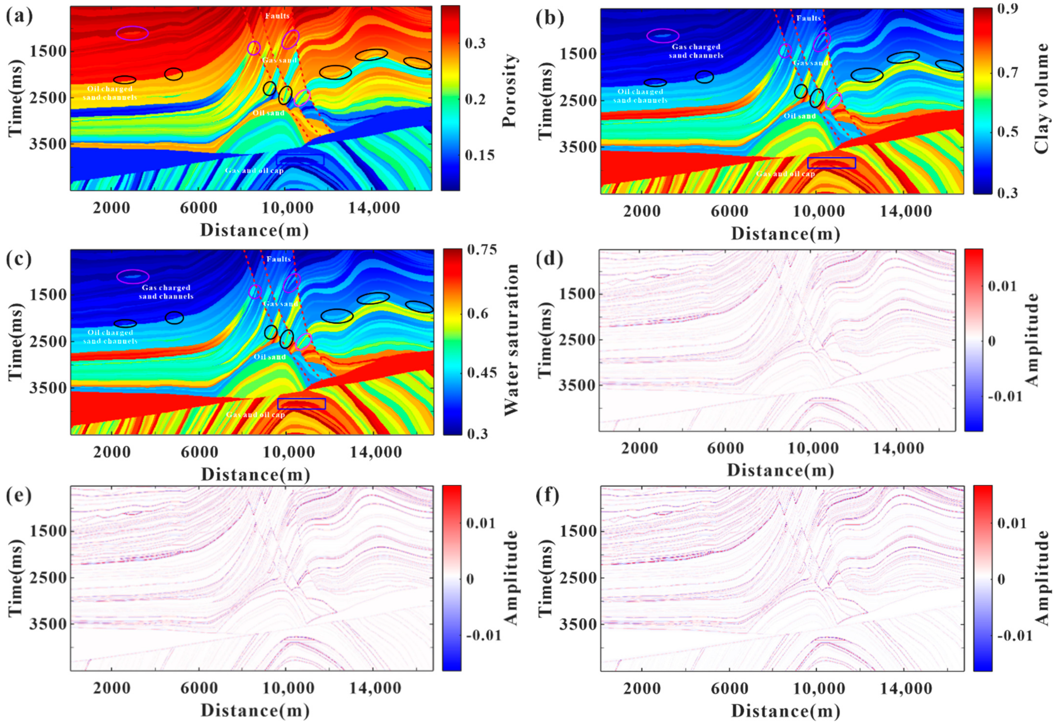
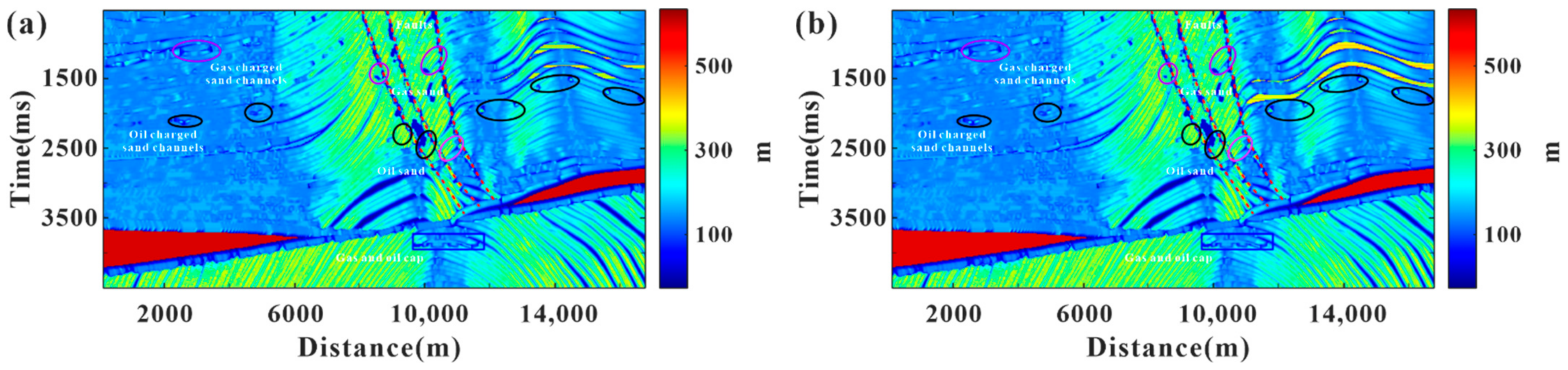
Martin [31] divided the structural elements, horizons, and lithologies of the Marmousi2 model. To further test the estimation effectiveness of the non-stationary random medium parameters proposed in this research, we used a part of the Marmousi2 model for the test. We selected the part of the original Marmousi2 model with a vertical time range of 501–4503 ms and a horizontal distance range of 101–16,900 m for the test. Based on the linearized petrophysical model, porosity, clay volume, and water saturation models were calculated from p-wave velocity, s-wave velocity, and density. Figure 9a–c display the porosity, clay volume, and water saturation of the Marmousi2 model, respectively. The model contained special geological bodies, such as a gas-charged sand channel, oil-charged sand channel, and large faults. The Ricker wavelet was set with the dominant frequency of 35 Hz, and Figure 9d–f are synthetic seismic records with central angles of 7°, 18°, and 26°, respectively. The non-stationary random medium parameters of porosity, clay volume, and water saturation were estimated based on the proposed method, and the parameter estimation results are depicted in Figure 10.
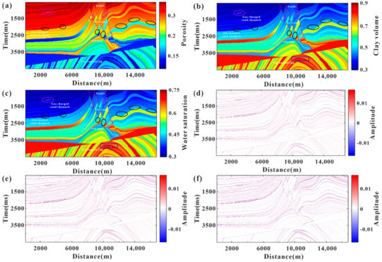
Figure 9.
Part of Marmousi2 model data and seismic data from different center angles: (a) porosity, (b) clay volume, (c) water saturation, (d) 7°, (e) 18°, (f) 26°.
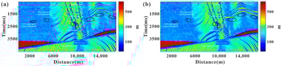
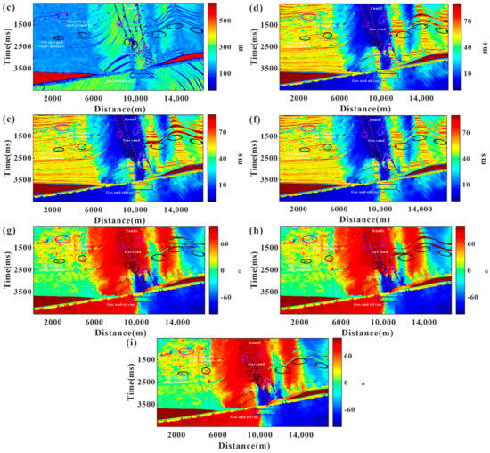
Figure 10.
Estimation results of autocorrelation parameters of porosity, clay volume, and water saturation: (a–c) are the horizontal autocorrelation length of porosity, clay volume, and water saturation, respectively. (d–f) are the vertical autocorrelation length of porosity, clay volume, and water saturation, respectively. (g–i) are the autocorrelation angle of porosity, clay volume, and water saturation, respectively.
The horizontal autocorrelation length is first analyzed. In the gas-charged sand channel and oil-charged sand channel, the autocorrelation lengths of the petrophysical parameters are smaller than those of the surrounding geological bodies, and there are areas with more obvious low values. The autocorrelation length of the petrophysical parameters will not show a small autocorrelation length throughout the sand. However, there will be a region with a more obvious low value at the edge of the two ends of these sands. In the gas and oil cap, the autocorrelation length of this geologic body is smaller than that of the surrounding geologic body, and there are also more obvious areas, with low values, at the edges of both ends of this geologic body.
Next, the vertical autocorrelation length is analyzed. There is no significant change in the autocorrelation length of these geologic bodies, and the autocorrelation length is smaller only at the edge positions of the two ends of the geologic bodies. This is because the distribution of these geologic bodies in the vertical direction is similar to that of other geologic bodies, and at the edge locations, the scale of the vertical direction decreases, and the length of the vertical autocorrelation diminishes. In the gas and oil cap, the scale of this geological body is more obviously different from other geological bodies, and its vertical scale is thicker; thus, the corresponding vertical autocorrelation length of petrophysical parameters is also larger. At the fault location, the horizontal and vertical autocorrelation lengths of the petrophysical parameters are smaller than those of the surrounding geological bodies, and they present low values.
Finally, the autocorrelation angle is analyzed. The autocorrelation angle is consistent with the change of the dip angle of the geological body, which varies with the change of the geological body and shows a positive correlation. In the unconformable salt rock, because the scale and thickness of its geological body are much larger than those of the surrounding geological bodies, the obtained autocorrelation length and autocorrelation angle both show large values. Autocorrelation length and autocorrelation angle, between porosity, clay volume, and water saturation, do not differ significantly. These three petrophysical parameters are closely related to the scale and elastic properties of their corresponding geological bodies, so their autocorrelation lengths and autocorrelation angles are within a large scale range, with smaller variations on small scales. The process of solving for the autocorrelation parameter defines a sliding window for the autocorrelation parameter, leading to a smoothing effect on the resulting autocorrelation parameter. To enhance the accuracy of parameter estimation at small geologic bodies, the size of the sliding window is adapted to the prediction of random medium parameters at small geologic bodies but not at large geologic bodies. Therefore, the estimation results of random medium parameters have large errors at unconformable salt rocks.
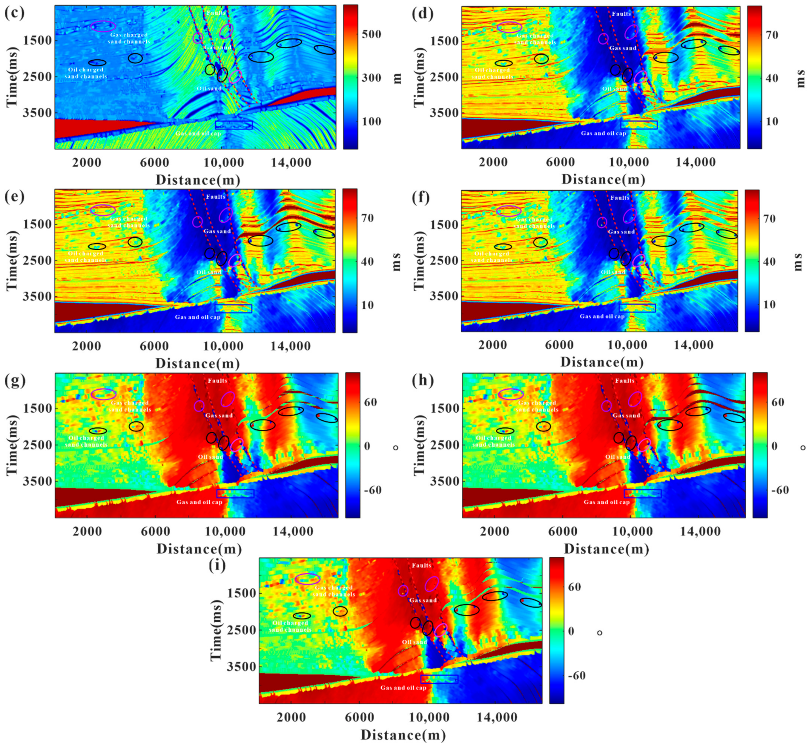
To illustrate the estimation effectiveness of the proposed method, we estimated the autocorrelation parameters directly from the porosity, clay volume, and water saturation models. Figure 11 shows the estimation results of autocorrelation parameters directly from the model. Compared with the autocorrelation parameters estimated directly using the model, the estimation result of the autocorrelation parameters, based on partially stacked seismic data, is smoother. Although there are deviations in the local details of the parameter estimation results, the overall trend estimated by the proposed method can match the results estimated directly by using the model. For the sand bodies in the three black elliptical boxes on the right side of the model, the boundaries of these three geological bodies in the petrophysical parameter model correspond to the regions of small values of the horizontal and vertical autocorrelation lengths of the petrophysical parameters. Therefore, the results of autocorrelation parameter estimation can reflect the variation of porosity, clay volume, and water saturation, in different geological bodies, more intuitively, and they can be a reference for interpreters.
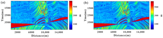

Figure 11.
Estimation results of autocorrelation parameters directly from the model: (a–c) are the horizontal autocorrelation length of porosity, clay volume, and water saturation, respectively. (d–f) are the vertical autocorrelation length of porosity, clay volume, and water saturation, respectively. (g–i) are the autocorrelation angle of porosity, clay volume, and water saturation, respectively.
4. Field Data Example
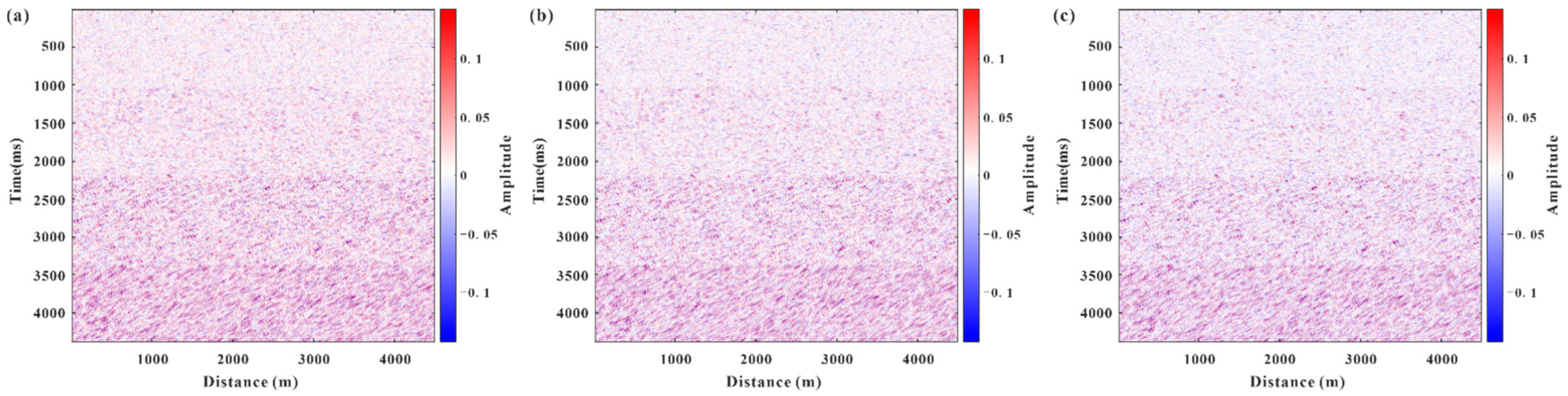
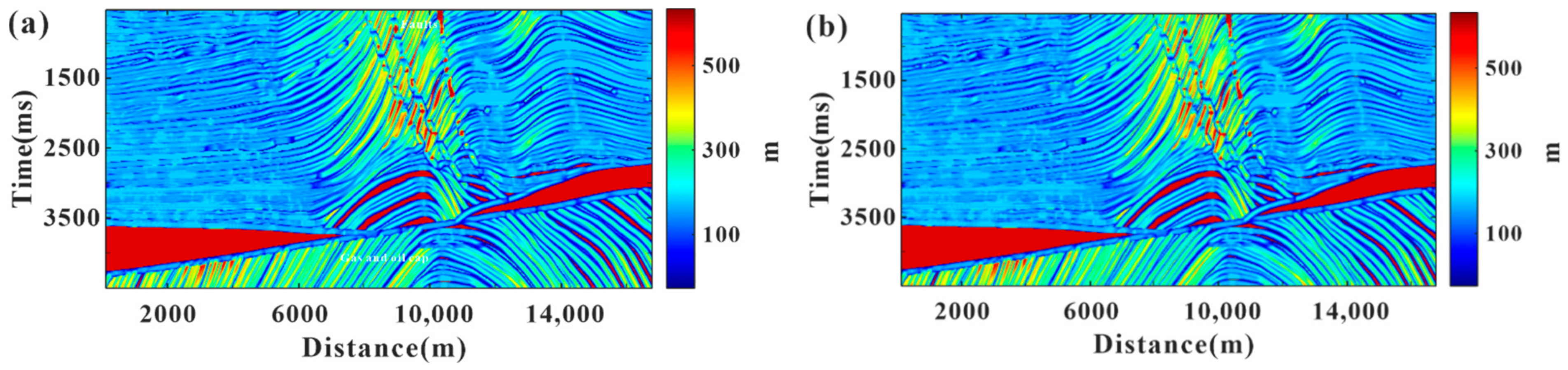
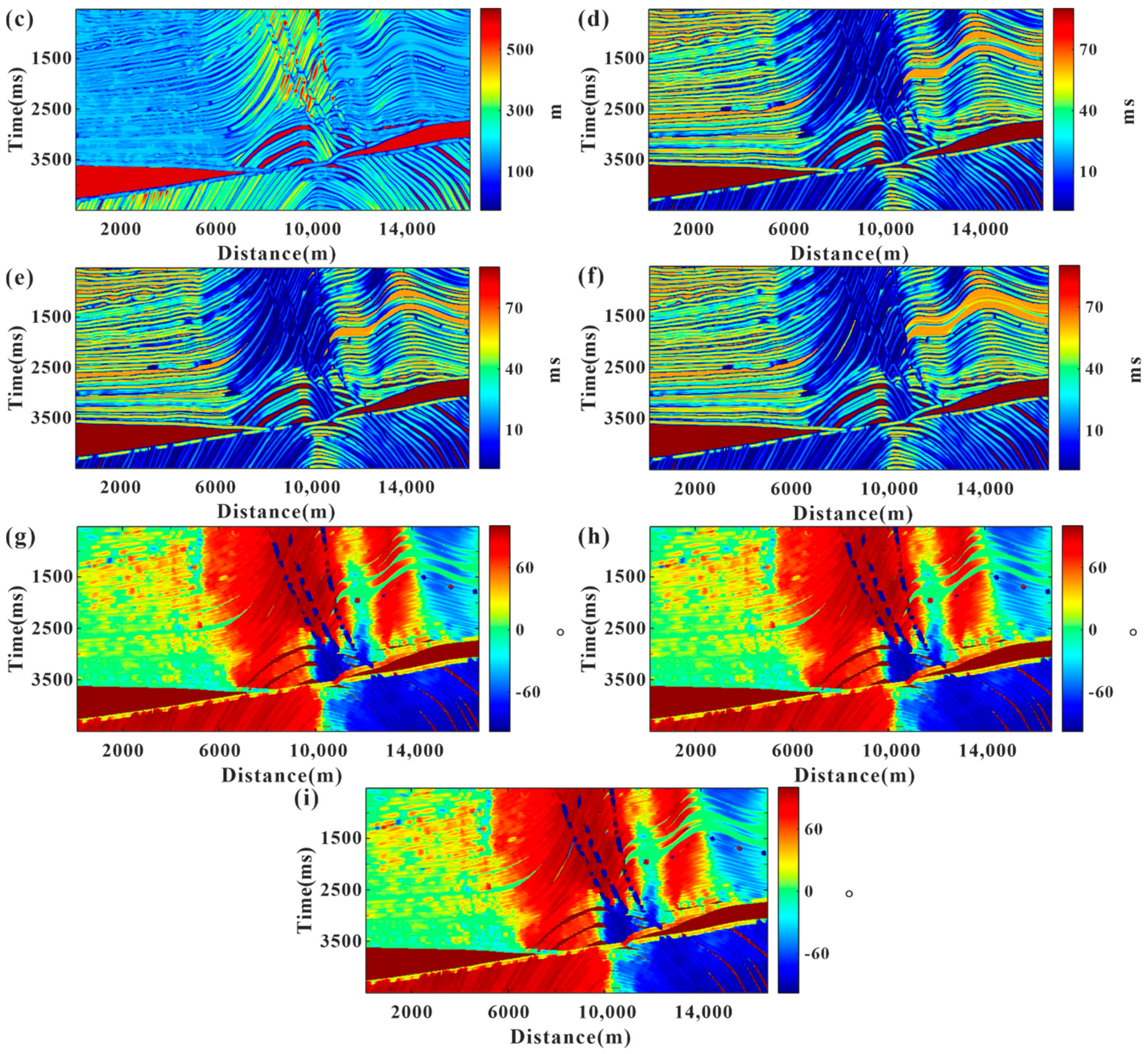
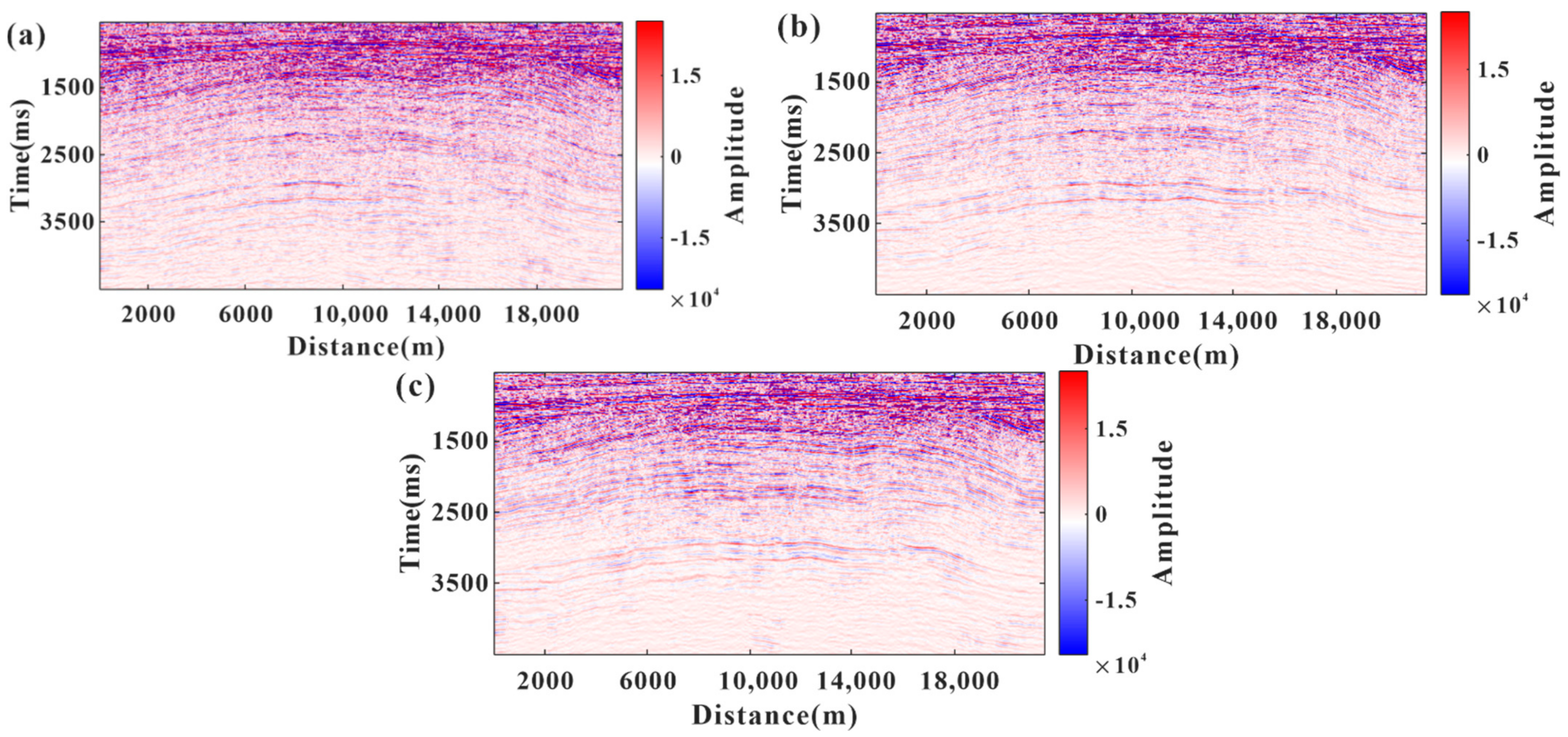
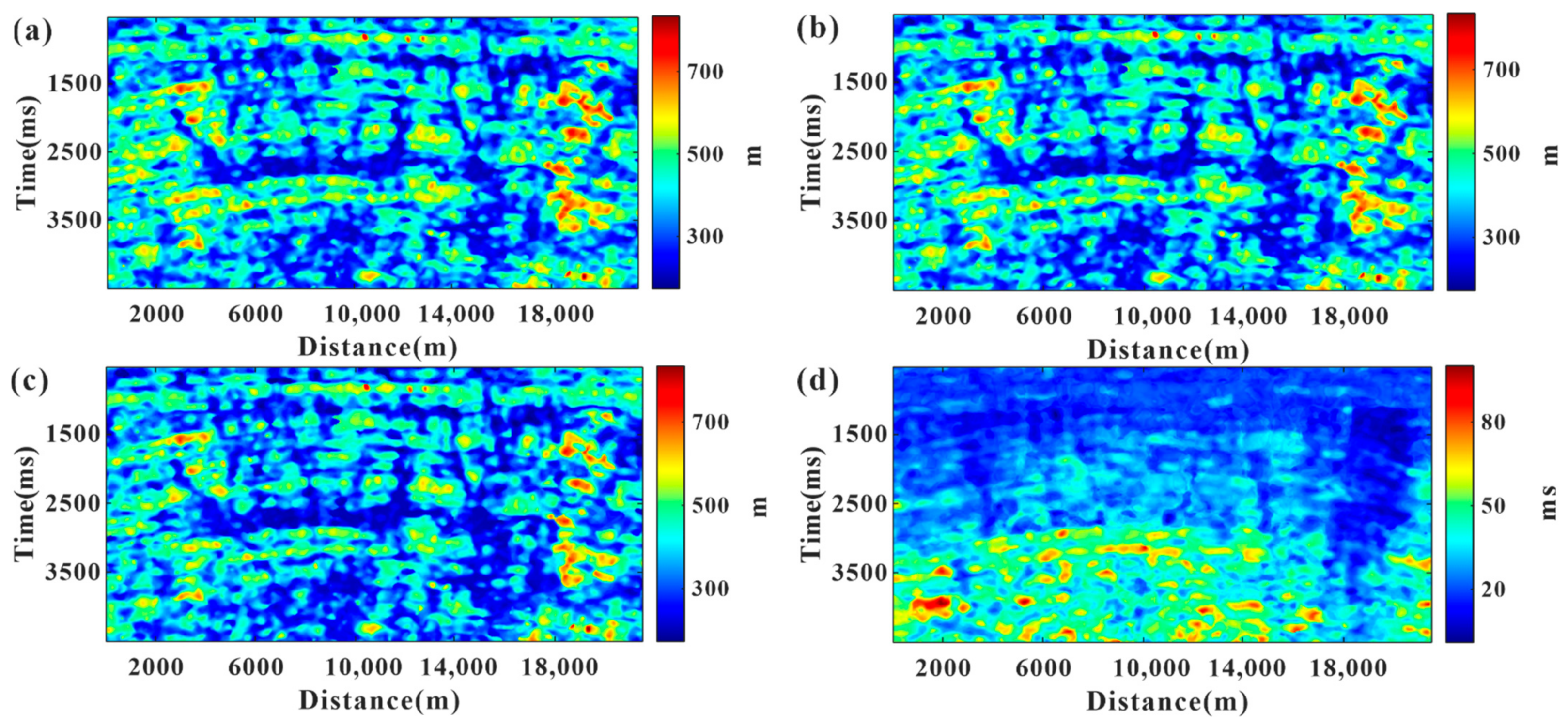
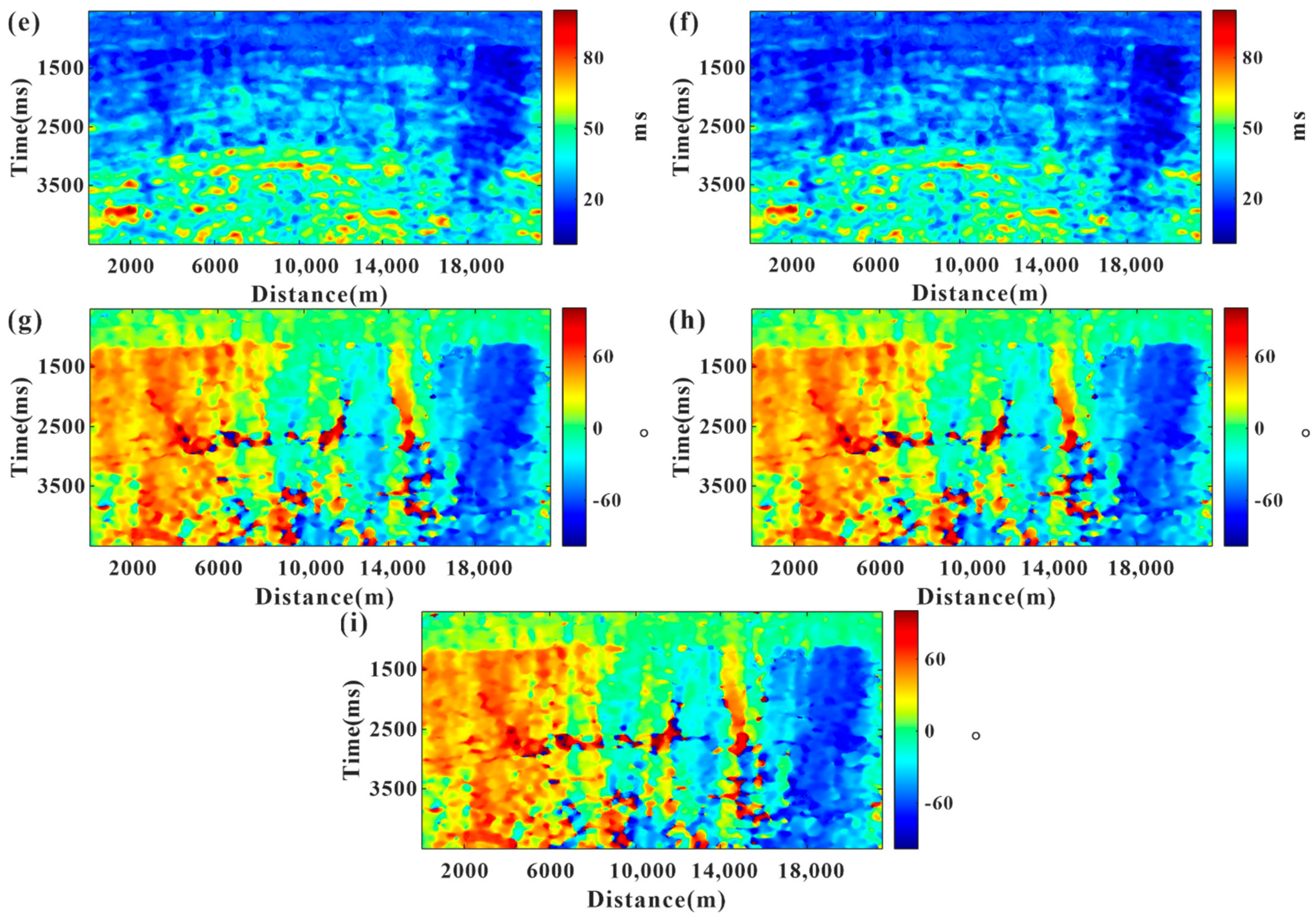
To further evaluate the effectiveness of the proposed method, for estimating the non-stationary random medium parameters of petrophysical parameters in field data, the data from an actual work area, in an oil field located in eastern China, were selected for testing. The work area is an anticline trap, and the main lithology is tight sandstone. Figure 12 exhibits the stacked seismic data with center angles of 7°, 15°, and 24°, respectively. Random medium autocorrelation parameters of porosity, clay volume, and water saturation were estimated by combining stacked seismic data from different center angles. Figure 13 illustrates the results of estimating the random medium autocorrelation parameters of porosity, clay volume, and water saturation. For positions with small structural changes and gentle positions, the horizontal autocorrelation length and vertical autocorrelation length of petrophysical parameters did not change much. At the positions with undulating and changing structures, the horizontal autocorrelation lengths of the three petrophysical parameters showed large values, and the vertical autocorrelation lengths showed small values. The autocorrelation angle of the petrophysical parameters varied with the dip angle of the subsurface medium. There were minor differences in the length and angle of autocorrelation between porosity, clay volume, and water saturation, but the overall trend was consistent. This also indicated that the variations of the random medium autocorrelation parameters for different petrophysical parameters of the subsurface medium, in the same structural geological body, are similar on large scales and different on small scales.

Figure 12.
Stacked seismic data with different center angles: (a) 7°, (b) 15°, (c) 24°.
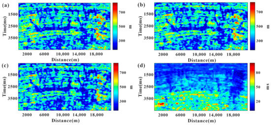
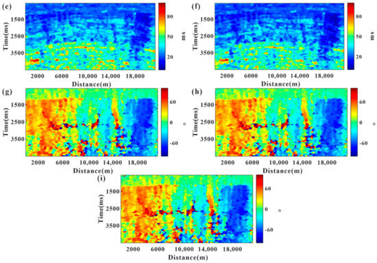
Figure 13.
Estimation results of autocorrelation parameters of porosity, clay volume, and water saturation: (a–c) are the horizontal autocorrelation length of porosity, clay volume, and water saturation, respectively. (d–f) are the vertical autocorrelation length of porosity, clay volume, and water saturation, respectively. (g–i) are the autocorrelation angle of porosity, clay volume, and water saturation, respectively.
5. Conclusions
The estimation of non-stationary random medium parameters of petrophysical parameters is the key to the application of random medium theory to fine seismic exploration. In this study, the relationship between the petrophysical and elastic parameters was constructed through a linear petrophysical model, and the relationships between the random medium porosity, clay volume, and water saturation models, as well as the power spectrum of seismic data were derived. Based on partial angle stacked seismic data, a method for estimating the physical parameters of a non-stationary random medium was proposed. The effect of parameter estimation, for a non-stationary random medium of petrophysical parameters, was analyzed by simple and complex model data tests, and the feasibility of the method was verified. Furthermore, we applied the method to estimate non-stationary random medium parameters of petrophysical parameters for field data. The power spectrum method, based on the Wiener–Khinchin theorem for the estimation of non-stationary random medium parameters, does not require iteration through inversion, which has the advantage of being intuitive and efficient. The method estimates the petrophysical parameters by using non-stationary random medium parameters from partial angle stacked seismic data, and it can simultaneously estimate nine characteristic parameters of porosity, clay volume, and water saturation in horizontal and vertical autocorrelation lengths and autocorrelation angles. This study can be applied to the initial model construction of the pre-stack seismic inversion of porosity, clay volume, and water saturation to provide a reference initial model for the inversion. However, the method requires setting the size of the sliding window, which has a smoothing effect that leads to an error with the real random medium parameters, and therefore, it needs further improvement.
Author Contributions
Conceptualization, Y.L. and G.Z.; methodology, Y.L. and G.Z.; software, Y.L. and G.Z.; validation, Y.L., G.Z., M.H., B.W. and S.C.; formal analysis, Y.L., G.Z. and B.W.; investigation, Y.L., G.Z. and M.H.; resources, Y.L. and G.Z.; data curation, Y.L., G.Z. and S.C.; writing—original draft preparation, Y.L.; writing—review and editing, Y.L., G.Z., M.H. and B.W. All authors have read and agreed to the published version of the manuscript.
Funding
This research was funded by National Natural Science Foundation of China, grant number 42174144, 42074136 and U19B2008, the PetroChina Prospective, Basic, and Strategic Technology Research Project, grant number 2021DJ0606, and the Fundamental Research Funds for the Central Universities, grant number 19CX02007A.
Data Availability Statement
Data sharing not applicable. The data used to support the findings of this study have not been made available because the author did not obtain permission to share the data.
Acknowledgments
We would like to sincerely thank the editor and reviewers for their helpful and constructive comments that clearly contributed to improving this article.
Conflicts of Interest
The authors declare no conflict of interest.
Appendix A
The contents of this appendix show the detailed derivation process of Equation (6) to Equation (9).
Substituting Equations (4) and (5) into Equation (6) yields the following equation:
Simplify Equation (A1) to obtain the relative disturbances of the p-wave velocity, s-wave velocity, and density.
According to the elastic impedance equation published by Connolly on The Leading Edge in 1999, the reflection coefficient can be expressed as follows:
where EI indicates elastic impedance and denotes incidence angle, .
Substitute Equation (4) into Equation (A3) to earn the following formula:
In the study of the non-stationary random medium model, we assume that the random medium is stationary throughout a small local range of the model. For the stationary random medium model, the background p-wave velocity, background s-wave velocity, and background density are all constants. Then,
Therefore, Equation (A4) can be written as:
Because , , and stand for small-scale disturbances, their values are small, thus, we have:
And because , Equation (A8) can be written as follows:
For partial angle stacked seismic data in the time domain, the seismic record can be approximated as the convolution of the reflection coefficient and the seismic wavelet as follows:
Substitution of Equation (A9) into Equation (A10) yields the following equation:
According to the differential properties of convolution, the following equation is obtained:
At this time, let:
Substitution of Equation (A2) into Equation (A14) yields the following equation:
Simplification of Equation (A15) yields the following equation:
Let:
Then, Equation (A16) can be expressed as:
Substitution of Equation (A18) into (A12) results in the following equation:
Then, the power spectrum of Equation (A19) can be expressed as follows:
The total power spectrum of the random medium can be expressed as:
When the total power spectrum of the random medium is obtained, the total autocorrelation function of the random medium can be achieved by performing the inverse Fourier transform on it.
According to Equation (A18), the total power spectrum of the random medium can also be expressed as follows:
Therefore, the partially stacked seismic data from three angles can be used to calculate the autocorrelation function of porosity, clay volume, and water saturation, respectively.
where symbolizes the Fourier transform results of at different incidence angles, respectively. signify the coefficients at different incidence angles, and indicates the Fourier transformed data of B at different incidence angles.
Equation (A23) can be written in matrix form as follows:
Thus, the power spectrum of porosity , clay volume , and water saturation is expressed as follows:
where is Hadamard product. Then,
Therefore, according to the Wiener–Khinchin theorem, the autocorrelation function of porosity , clay volume , and water saturation can be procured by doing the Fourier inverse transformation on the power spectrum data.
References
- Aki, K. Analysis of the seismic coda of local earthquakes as scattered waves. J. Geophys. Res. 1969, 74, 615–631. [Google Scholar] [CrossRef]
- Ikelle, L.; Yung, S.; Daube, F. 2-D random media with ellipsoidal autocorrelation functions. Geophysics 1993, 58, 1359–1372. [Google Scholar] [CrossRef]
- Levander, A.; England, R.W.; Smith, S.K.; Hobbs, R.W.; Goff, J.A.; Holliger, K. Stochastic characterization and seismic response of upper and middle crustal rocks based on the Lewisian gneiss complex, Scotland. Geophys. J. Int. 1994, 119, 243–259. [Google Scholar] [CrossRef] [Green Version]
- Hurich, C.A.; Kocurko, A. Statistical approaches to interpretation of seismic reflection data. Tectonophysics 2000, 329, 251–267. [Google Scholar] [CrossRef]
- Gu, Y.; Zhu, P.M.; Li, H.; Li, X.Y. Stationary random medium parameter estimation of two-dimensional post-stack seismic data. Chin. J. Geophys. 2014, 57, 2291–2301. [Google Scholar]
- Gibson, B.S. Analysis of lateral coherency in wide-angle seismic images of heterogeneous targets. J. Geophys. Res. Solid Earth 1991, 96, 10261–10273. [Google Scholar] [CrossRef]
- Poppeliers, C. Estimating vertical stochastic scale parameters from seismic reflection data: Deconvolution with non-white reflectivity. Geophys. J. Int. 2007, 168, 769–778. [Google Scholar] [CrossRef] [Green Version]
- Saito, T.; Sato, H.; Ohtake, M. Envelope broadening of spherically outgoing waves in three-dimensional random media having power law spectra. J. Geophys. Res. Solid Earth 2002, 107, ESE-3. [Google Scholar] [CrossRef] [Green Version]
- Meng, X.; Wang, S.; Tang, G.; Li, J.; Sun, C. Stochastic parameter estimation of heterogeneity from crosswell seismic data based on the Monte Carlo radiative transfer theory. J. Geophys. Eng. 2017, 14, 621–633. [Google Scholar] [CrossRef]
- Carpentier, S.F.A.; Roy-Chowdhury, K. Conservation of lateral stochastic structure of a medium in its simulated seismic response. J. Geophys. Res. Solid Earth 2009, 114, B10. [Google Scholar] [CrossRef] [Green Version]
- Irving, J.; Knight, R.; Holliger, K. Estimation of the lateral correlation structure of subsurface water content from surface-based ground-penetrating radar reflection images. Water Resour. Res. 2009, 45, 1–14. [Google Scholar] [CrossRef]
- Scholer, M.; Irving, J.; Holliger, K. Estimation of the correlation structure of crustal velocity heterogeneity from seismic reflection data. Geophys. J. Int. 2010, 183, 1408–1428. [Google Scholar] [CrossRef] [Green Version]
- Gu, Y. Numerical Modeling and Parameter Estimation for 3D Non-Stationary Random Medium. Ph.D. Thesis, China University of Geosciences, Wuhan, China, 2013. [Google Scholar]
- Jeulin, D. Dead Leaves Models: From Space Tessellations to Random Functions; Springer: Cham, Switzerland, 2021; Volume 53, pp. 329–418. [Google Scholar]
- Bakulin, A.; Grechka, V.; Tsvankin, I. Estimation of fracture parameters from reflection seismic data—Part II: Fractured models with orthorhombic symmetry. Geophysics 2000, 65, 1803–1817. [Google Scholar] [CrossRef] [Green Version]
- Zhang, L.; Xu, Y.; Zeng, Z.; Li, J.; Zhang, D. Simulation of Martian Near-Surface Structure and Imaging of Future GPR Data from Mars. IEEE Trans. Geosci. Remote Sens. 2021, 21, 1–11. [Google Scholar] [CrossRef]
- Yan, F.; Han, D.H. Accuracy and sensitivity analysis on seismic anisotropy parameter estimation. J. Geophys. Eng. 2018, 15, 539–553. [Google Scholar] [CrossRef] [Green Version]
- Carpentier, S.F.A.; Roy-Chowdhury, K.; Hurich, C.A. Mapping correlation lengths of lower crustal heterogeneities together with their maximum-likelihood uncertainties. Tectonophysics 2011, 508, 117–130. [Google Scholar] [CrossRef]
- Yang, X.W.; Zhu, P.M. Stochastic seismic inversion based on an improved local gradual deformation method. Comput. Geosci. 2017, 109, 75–86. [Google Scholar] [CrossRef]
- Yang, X.W.; Mao, N.B.; Zhu, P.M.; Xiao, D. Two-level uncertainty assessment in stochastic seismic inversion based on the gradual deformation method. Geophysics 2020, 85, M33–M42. [Google Scholar] [CrossRef]
- Fan, Y.; Lu, Q.T.; Feng, J.; Zhang, J.; Luo, S.Y. Estimation of lateral correlation length from deep seismic reflection profile based on stochastic model. Acta Geophys. 2021, 69, 1297–1312. [Google Scholar]
- Wang, B.L.; Lin, Y.; Zhang, G.Z.; Yin, X.Y.; Zhao, C. Prestack seismic stochastic inversion based on statistical characteristic parameters. Appl. Geophys. 2021, 18, 63–74. [Google Scholar]
- Litwiniszyn, J. Application of the equation of stochastic processes to spatial problems of mechanics of some types of bodies. Bull. L’Academie Pol. Des. Sci. 1956, 4, 91–95. [Google Scholar]
- Xi, X.; Yao, Y. Simulations of Random Medium Model and Intermixed Random Medium. J. China Univ. Geosci. 2002, 27, 67–71. [Google Scholar]
- Xi, X.; Yao, Y. 2-D random media and wave equation forward modeling. Oil Geophys. Prospect. 2001, 36, 546–552. [Google Scholar]
- Xi, X.; Yao, Y. Non-stationary random medium model. Oil Geophys. Prospect. 2005, 40, 71–75. [Google Scholar]
- Yin, X.Y.; Cui, W.; Zong, Z.Y.; Liu, X.J. Petrophysical property inversion of reservoirs based on elastic impedance. Chin. J. Geophys. 2014, 57, 4132–4140. [Google Scholar]
- Zhang, J.J.; Yin, X.Y.; Zhang, G.Z.; Gu, Y.P.; Fan, X.G. Prediction method of physical parameters based on linearized rock physics inversion. Pet. Explor. Dev. 2020, 47, 59–67. [Google Scholar] [CrossRef]
- Grana, D. Bayesian linearized rock-physics inversion. Geophysics 2016, 81, D625–D641. [Google Scholar] [CrossRef]
- Connolly, P. Elastic impedance. Lead. Edge 1999, 18, 438–452. [Google Scholar] [CrossRef]
- Martin, G.S.; Wiley, R.; Marfurt, K.J. Marmousi2: An elastic upgrade for Marmousi. Lead. Edge 2006, 25, 156–166. [Google Scholar] [CrossRef]


Publisher’s Note: MDPI stays neutral with regard to jurisdictional claims in published maps and institutional affiliations. |
© 2022 by the authors. Licensee MDPI, Basel, Switzerland. This article is an open access article distributed under the terms and conditions of the Creative Commons Attribution (CC BY) license (https://creativecommons.org/licenses/by/4.0/).