Analysis of Light Utility Vehicle Readiness in Military Transportation Systems Using Markov and Semi-Markov Processes

Abstract

This paper presents the issues of modeling the operation process of light utility vehicles operating in military transport systems. The required condition for the effective operation of the system is to maintain the means of transport at the appropriate level of technical readiness. For this purpose, it is necessary to equip the technical system with appropriate resources enabling the efficient implementation of fuel refilling, maintenance and repair processes. Each failure of the means of transport causes a significant reduction in transport capacity, which then results in the inability to perform the planned tasks. Quality control and vehicle operation process management require advanced mathematical methods and tools. Three indicators have been proposed as quantitative characteristics for assessing and optimizing the availability of military vehicles: functional readiness, technical efficiency and airworthiness. To determine their value, a stochastic exploitation model was developed based on the application of the theory of Markov processes. Based on the collected empirical data, a nine-state phase space of the studied process was identified. Operating states were distinguished relating to the implementation of the transport task, refueling, parking in the garage, as well as maintenance and repairs. As part of the considerations for the continuous time, verification of the distributions of time characteristics led to the development of a semi-Markov model. The ergodic probabilities calculated based on the conditional probability matrix of interstate transitions and the expected values of the time spent in the states were used to determine the indicators of functional availability, efficiency and technical suitability. In order to determine the possibility of optimizing the process, a sensitivity analysis was performed. Reducing the amount of time the vehicles must wait for repair by about 50% can improve the values of the indexes from 0.91 to 0.95.

1. Introduction

Military transport systems aim to ensure that transport capacity corresponds to the existing needs. The determinants of the level of transport needs include combat operations, training plans and the current activity of military units. The fleet of reliable vehicles is one of the main factors determining the high quality and timely implementation of processes in modern transport systems. The condition for the effective operation of the system is to maintain the means of transport in a state of technical efficiency and be ready to perform tasks [1,2]. The fulfilment of this condition is possible thanks to the organization of operating systems with appropriate technical resources to carry out processes of diagnosis, servicing and repair of vehicles. Along with the increase in the intensity of the use of means of transport, the demand for fuel and other consumables increases significantly, especially in the case of military vehicles traveling outside the area of public roads [3,4,5].

Military exploitation systems are largely based on a plan-preventive maintenance strategy, aiming to maximize the technical availability of facilities [6,7,8,9]. This strategy assumes the implementation of maintenance with a specific labor intensity, in accordance with the required scope. The guidelines for maintenance activities, time intervals and the size of the service life between maintenance are defined based on the manufacturer’s technical specifications and the knowledge and experience of specialists dealing with planning and standardization of operation at individual management levels. The main disadvantages of this strategy are its cost-intensive nature and low flexibility.

The operation process covers activities related to a technical object from the moment of its production to its liquidation. During this period, there are essentially two overlapping sub-processes usage and maintenance. The rational use of machines and devices allows for extending the intervals between subsequent maintenance services, recreating the technical service life of the facility, and also reducing the current operating costs. The model of the operation process should, on the one hand, reflect the basic technical characteristics of the object consistent with the modeling objective, and on the other hand, it should be used for the rational forecasting of use and maintenance [10,11,12,13].

Markov’s theory has found applications in many fields of science and technology. There are many scientific studies in the literature on the use of Markov processes for reliability modeling [14,15], the operation of objects [16,17,18,19] and technical systems [20,21]. Depending on the case study and the purpose of modeling, the authors constructed models based on a diverse number of operational states in the phase space. The least complicated Markov chain model was presented in [22] and applied to simulate and optimize energy savings for machines operating in production systems. Models with three states were constructed to analyze and assess the technical availability of buses [23], special vehicles [24], operational readiness of wind turbine elements [17], working time of production machines [25], the time interval of preventive maintenance [26] and the reliability of technical facilities [27]. In [28], the authors developed a five-state semi-Markov model with the Weibull distribution of the residence times of four types of buses in the states of the renewal process. This model allowed for profit optimization per unit of time and availability depending on the duration of preventive maintenance.

The comparison of the values obtained by the six-state Markov and semi-Markov models, which the authors of the publication [29] developed for production machines, indicated that the unverified assumption of the exponential distribution of the time the object stays in states may lead to significant errors in the calculation of the readiness indices. In the presented case study, the difference between the results of the semi-Markov model and the erroneous Markov model was as much as 0.40, which is less than half of the actual value of the readiness index.

Markov models with 9- and 16-state phase spaces are presented in [8,30] with much more elaborate models. The increased number of states allows a detailed analysis of the process and factors affecting the technical readiness of the facility. The multi-state models presented in [31] accurately reflected the stochastic nature of the electric vehicle driving cycle during their use in urban areas, outside the city, on the motorway and during road congestion.

Table 1. Literature review of Markov and semi-Markov modeling in engineering.

Paper	Case Study	Model	Results and Conclusions
[22]	Machines in manufacturing system	Two-state Markov chain	The model was developed to simulate and optimize energy saving.
[8]	Military helicopters	Nine-state Markov model	Boundary probabilities were calculated for all states and the functional readiness index reached 0.9223.
[17]	Spring shock absorber in wind turbine system	Three-state semi-Markov model of maintenance	Erlang distribution of sojourn time. The system operational availability reached 0.6354–0.6497.
[25]	Machines in wafer fabrication work centre	Three-state hidden semi-Markov model	Accuracy of the machine condition recognition was 95.56% and prediction accuracy of job processing time was 94.91%.
[29]	Production machines	Six-state Markov and semi-Markov models	Readiness index: 0.85 (semi-Markov model) and 0.45 (Markov model). Groundless assumption of exponential distribution lead to incorrect results.
[24]	Special vehicles	Three-state semi-Markov model	Technical readiness factor was 0.95.
[30]	Means of transport	16-state semi-Markov model of exploitation process	Genetic algorithm was proposed for determining the optimal strategy to control availability.
[23]	Buses in transportation system	Three-state hidden Markov model	Probability of availability reached values in the range 0.896–0.969.
[28]	Four types of city bus renewal processes	Five-state semi-Markov model (Weibull distribution)	The model allows to optimize the profit per unit time and readiness to carry out transport tasks depending on the time to preventive maintenance.
[27]	Reliability of technical objects	Three-state semi-Markov model	Reliability function for Poisson and Furry-Yule failure rate processes.
[26]	Marine diesel engines	Three-state semi-Markov model (Weibull distribution)	The optimal preventive maintenance interval was 1095 h.
[31]	Driving cycles of electric vehicles	Multistate Markov models of acceleration	The models describe the stochastic nature of driving cycles in four scenarios: rural, highway, urban and congestion.
[19]	Offshore wind farms	Six-state Markov model	The proposed method allows for improving maintenance efficiency of offshore wind farms.
[10]	Transformers	Five-state Markov chain	Prediction of maintenance cost in 20-year forecast horizon.

summarizes the literature review containing the latest publications in the field of modeling the exploitation process with the use of Markov theory.

In this publication, the authors addressed the issue related to the operation of light utility vehicles operating in military transport systems. The research sample consisted of 19 Honker vehicles for which detailed data were collected during the three-year research period. The operating system is focused on maintaining the high reliability of vehicles through an appropriately planned and implemented maintenance strategy. The plan-preventive system each time assumes the scope of maintenance works after a specified amount of work (mileage) or time elapsed. Unfortunately, the records of operation are still kept in the form of traditional documentation registered on an ongoing basis by direct users (drivers) and in relation to inspections and repairs by service and repair workshops. Source documents that create departure orders, technical service cards and operation plans were used to prepare detailed databases individually for each facility.

The current review of the literature allows the authors to state there are no studies on the analysis and evaluation of the operation of heavy goods vehicles with the use of the Markov theory. It was a premise for conducting scientific research and developing an exploitation model for the aforementioned group of military vehicles. In addition, Honker vehicles have a significant share in the structure of the military transport fleet of the Polish Armed Forces. Carrying out the modeling of the operation process based on the application of the Markov theory requires a thorough understanding of the examined process and enables the analysis and assessment of the basic operational indicators of the studied object.

This article presents the original methodology for creating a stochastic model of Honker vehicles based on the Markov theory. An algorithm for creating a mathematical model was developed, the practical usefulness of which was verified on the actual operation process of the said sample of vehicles. An event model covering the nine-state phase space of the process was developed. The determined values of ergodic probabilities for individual operational states constituted the basis for calculating the values of functional availability, efficiency and technical suitability indicators. From the point of view of the transport capacity of the entire system as well as economic and technical conditions, the personnel managing the vehicle operation process aim to maximize the presented readiness and/or reliability measures. The proposed methodology makes it possible to indicate possible components influencing the improvement of exploitation indicators. The performed sensitivity analysis of the model allows for the examination of the impact of improving the organization of the repair subsystem, consisting of the shortening/elimination of waiting time for spare parts, on the readiness indicators of the tested sample of vehicles.

The nine-state model adds to the current state of the literature both in terms of the subject of the study and the application of sensitivity analysis to identify opportunities for improving process efficiency. No previous scientific studies have addressed the issue of modeling the operation of light utility vehicles (trucks) using Markov and semi-Markov process theory. In addition, a completely novel way of analyzing the sensitivity of the semi-Markov model in terms of the dependence of the values of ergodic probabilities on the values of expected dwell times was proposed.

The article has been divided into the following main chapters. The introduction reviews the current state of knowledge on the application of Markov theory to the exploitation process. Section 2 describes the methodology of creating event-based models of the operation process using the Markov theory. Section 3 provides a statistical analysis of the source data constituting the basis for the development of the model. In Section 4, the semi-Markov model is described, and the process research results are presented together with the model sensitivity analysis. The values of ergodic probabilities of the semi-Markov model were confronted with the standard Markov model. Finally, the Section 5 includes the conclusions from the conducted research.

2. Methods

The actual operation processes are a composition of deterministic and random sub-processes. Random components are usually interpreted as stochastic processes X(t) reflecting changes in the operational states of the tested object in discrete or continuous time. In the processes of exploitation at a random moment t, the object is only in one of the states identified in the phase space S = X(t). This assumption requires precise determination of all possible operational states in which vehicles may be in the course of the operation process. The stochastic processes fulfilling the Markov property are essential in terms of applicability. According to Markov’s theory, the conditional probabilities of reaching the future states X(t_z+1) result only from the current state X(t_z) [32]. Mathematically, this property is consistent with Equation (1) [33,34,35]:

$$P\left\{X\left(t_z\right)=x_z|X\left(t_{z-1}\right)=x_{z-1},X\left(t_{z-2}\right)=x_{z-2},\dots ,X\left(t_0\right)=x_0\right\}=P\left\{X\left(t_z\right)=x_z|X\left(t_{z-1}\right)=x_{z-1}\right\}.$$

(1)

The literature is dominated by the division of Markov processes with regard to time and state space, which distinguishes four types of processes, i.e., processes:

• Discrete in time and discrete in states;
• Continuous in time and discrete in states;
• Discrete in time and continuous in states;
• Continuous in time and continuous in states.

In operation, the most frequently used models are based on discrete processes in states, developed for both discrete and continuous time [8,16,24,28,29].

2.1. Markov Chains

The Markov chain assumes the discretization of time into specific Δt intervals, the width of which depends on the characteristics of the process, measurement technique, and, above all, the adopted modeling objective [36]. With the increase in the dynamics of the process course, the possibility, and, at the same time, the necessity to perform frequent measurements and the focus on creating a very accurate model, the values of time Δt decrease. The dynamics of changes in the operational states identified in the phase space for the operation of light utility vehicles determine the assumption of the duration of moments Δt for the time interval equal to 1 min. Increasing this value could cause the undesirable omission of registering the occurrence of conditions, which are usually short-lived. At the same time, reducing the time intervals is practically impossible due to recording the course of operation processes of vehicles operating in military transport systems.

Constructing the Markov Chain Model based on an empirical process flow requires acquiring data on interstate transitions. For this purpose, it is reasonable to create a matrix of the number of interstate transitions according to the Formula (2):

$$N=\left[\begin{array}{ccccc}{n}_{11}& n_{12}& \cdots & n_{1(k-1)}& n_{1k}\\ n_{21}& n_{22}& \cdots & n_{2(k-1)}& n_{2k}\\ ⋮& ⋮& \ddots & ⋮& ⋮\\ n_{(k-1)1}& n_{(k-1)2}& \cdots & n_{(k-1)(k-1)}& n_{(k-1)k}\\ n_{k1}& n_{k2}& \cdots & n_{k(k-1)}& n_{kk}\end{array}\right].$$

(2)

The values of the N matrix correspond to the total number of observed interstate transitions in the analyzed period of the process implementation, where n_ij is the transition from the i state to the j state.

For a homogenous Markov chain, the conditional probability p_ij of transition from state i to state j in one step is the same for every moment t. The homogeneity of the process indicates the invariability of the rules affecting the state changes at any time of its implementation. If the analyzed realizations of the process are included in the same phase of operation, then the course of the process should be homogenous. The probability values of the conditional interstate transitions are presented by means of the stochastic matrix P, according to the Formula (3) [33,37,38]:

$$P=\left[\begin{array}{ccccc}{p}_{11}& p_{12}& \cdots & p_{1(k-1)}& p_{1k}\\ p_{21}& p_{22}& \cdots & p_{2(k-1)}& p_{2k}\\ ⋮& ⋮& \ddots & ⋮& ⋮\\ p_{(k-1)1}& p_{(k-1)2}& \cdots & p_{(k-1)(k-1)}& p_{(k-1)k}\\ p_{k1}& p_{k2}& \cdots & p_{k(k-1)}& p_{kk}\end{array}\right],$$

(3)

provided that the following formula [37] is fulfilled:

$${\displaystyle \sum _{j=1}^k{p}_{ij}}=1.$$

(4)

The probabilities of the interstate transitions of the P stochastic matrix can be obtained using the values of the N interstate number matrix by estimation [31,35,39] according to the relationship:

$$p_{ij}=\frac{n_{ij}}{{\displaystyle \sum _{j=1}^k{n}_{ij}}},$$

(5)

where the standard error of the conditional probability estimation [40,41] is calculated according to the formula:

$$SE\left(p_{ij}\right)=\sqrt{\frac{p_{ij}\left(1-p_{ij}\right)}{{\displaystyle {\sum }_{j=1}^k{n}_{ij}}}}.$$

(6)

The values of ergodic probabilities π_j are calculated by solving the following matrix Equation (7) [37]:

$$(P^T-I)\cdot \Pi =0,$$

(7)

assuming that the normalization condition is met, according to the formula:

$${\displaystyle \sum _{j=1}^n{\pi }_j}=1.$$

(8)

2.2. Markov and Semi-Markov Processes

Discrete Markov models in states and continuous in time allow for the analysis of the operation process under constant supervision and monitoring of the course of changes in operational states. This approach excludes the influence of the size of the time moments Δt on the values of the instantaneous and ergodic characteristics of the process. In principle, the change of state from S_i to S_j can take place at any time during the process. It is also assumed that only one state change can occur at any time t. The Markov process assumes the presence of exponential distributions of the characteristics of individual states describing the analyzed process [42,43,44].

The transition intensity matrix Λ is the quantitative characteristic of the Markov process:

$$\Lambda =\left[\begin{array}{ccccc}{\lambda }_{11}& {\lambda }_{12}& \cdots & {\lambda }_{1(k-1)}& {\lambda }_{1k}\\ {\lambda }_{21}& {\lambda }_{22}& \cdots & {\lambda }_{2(k-1)}& {\lambda }_{2k}\\ ⋮& ⋮& \ddots & ⋮& ⋮\\ {\lambda }_{(k-1)1}& {\lambda }_{(k-1)2}& \cdots & {\lambda }_{(k-1)(k-1)}& {\lambda }_{(k-1)k}\\ {\lambda }_{k1}& {\lambda }_{k2}& \cdots & {\lambda }_{k(k-1)}& {\lambda }_{kk}\end{array}\right],$$

(9)

whose elements meet the following dependencies:

$$\forall i,j,i\ne j,{\lambda }_{ij}=\frac{d}{dt}{p}_{ij}=\underset{\Delta t\to 0}{\mathit{lim}}\frac{p_{ij}\left(t+\Delta t\right)-p_{ij}\left(t\right)}{\Delta t},$$

(10)

$$\forall i,{\lambda }_{ii}=-\frac{d}{dt}{p}_{ii}=\underset{\Delta t\to 0}{\mathit{lim}}\frac{1-\left(p_{ii}\left(t+\Delta t\right)-p_{ii}\left(t\right)\right)}{\Delta t}.$$

(11)

All elements of the matrix on the main diagonal have non-positive values, while all other elements are non-negative and the sum of all elements for each row of the transition intensity matrix is equal to 0.

In the operation processes of objects, the estimators of the values of the elements λ_ij of the interstate intensity matrix are the reciprocal of the average residence times in the S_i state before the transition to the S_j state. On the other hand, the value of λ_ii is taken as the reciprocal of the sum of the remaining elements in the i row. The presented description of the estimation of the intensity matrix elements can be written using the relationship:

$${\lambda }_{ij}=\frac{1}{T_{ij}},$$

(12)

$${\lambda }_{ii}=-{\displaystyle \sum _{j\ne i}{\lambda }_{ij}},$$

(13)

where T_ij is the average transition time from state S_i to state S_j.

The condition of exponential distributions of the stochastic process characteristics narrows the spectrum of applications of the Markov model in continuous time. Some characteristics of the operation process may not meet it. From the point of view of the reliability of the mapping, this excludes the possibility of applying the Markov model [29,45]. The generalization of the Markov process is the semi-Markov process, which does not require the fulfilment of the condition of exponential distributions of interstate transition times. In the semi-Markov process, the durations of states are independent random variables with any distribution function [27,43,46].

The basic characteristic of the semi-Markov process is the matrix of the renewal kernel Q(t), the elements of which are the products of the probability p_ij and the transition between the states S_i and S_j and the distribution function of the conditional duration distribution of the state S_i before the transition to S_j, according to the equation [30,47]:

$$Q\left(t\right)=\left[\begin{array}{ccccc}0& Q_{12}\left(t\right)& \cdots & Q_{1(k-1)}\left(t\right)& Q_{1k}\left(t\right)\\ Q_{21}\left(t\right)& 0& \cdots & Q_{2(k-1)}\left(t\right)& Q_{2k}\left(t\right)\\ ⋮& ⋮& \ddots & ⋮& ⋮\\ Q_{(k-1)1}\left(t\right)& Q_{(k-1)2}\left(t\right)& \cdots & 0& Q_{(k-1)k}\left(t\right)\\ Q_{k1}\left(t\right)& Q_{k2}\left(t\right)& \cdots & Q_{k(k-1)}\left(t\right)& 0\end{array}\right],$$

(14)

wherein:

$$Q_{ij}\left(t\right)=p_{ij}\cdot F_{ij}\left(t\right),$$

(15)

where p_ij is the probability of transition from the S_i state to S_j, and F_ij(t) is the distribution function of the residence time in state S_i before the transition to state S_j.

An embedded Markov chain is formulated for a semi-Markov process in continuous time, which represents changes in the process state without taking into account the residence times in individual states.

The embedded Markov chain assumes the possibility of transition from the S_i state to S_j, assuming that i ≠ j. The interstate transition probability matrix for such a chain can have non-zero elements only outside the main diagonal, which can be written by the formula:

$$P=\left[\begin{array}{ccccc}0& p_{12}& \cdots & p_{1(k-1)}& p_{1k}\\ p_{21}& 0& \cdots & p_{2(k-1)}& p_{2k}\\ ⋮& ⋮& \ddots & ⋮& ⋮\\ p_{(k-1)1}& p_{(k-1)2}& \cdots & 0& p_{(k-1)k}\\ p_{k1}& p_{k2}& \cdots & p_{k(k-1)}& 0\end{array}\right].$$

(16)

If the embedded Markov chain is ergodic and there are expected E(T_i) values of the times in individual states, then the ergodic values of the probabilities π_j for the semi-Markov process can be determined using the following dependencies:

$${\pi }_j=\frac{p_j\cdot E\left(T_j\right)}{{\displaystyle \sum _{i=1}^k{p}_i\cdot E\left(T_i\right)}},$$

(17)

$$E\left(T_j\right)={\displaystyle \sum _{i=1}^k{p}_{ij}{T}_{ij}},$$

(18)

where p_i is the ergodic probability of the embedded Markov chain for state S_i, and T_ij is the average transition time from state S_i to state S_j.

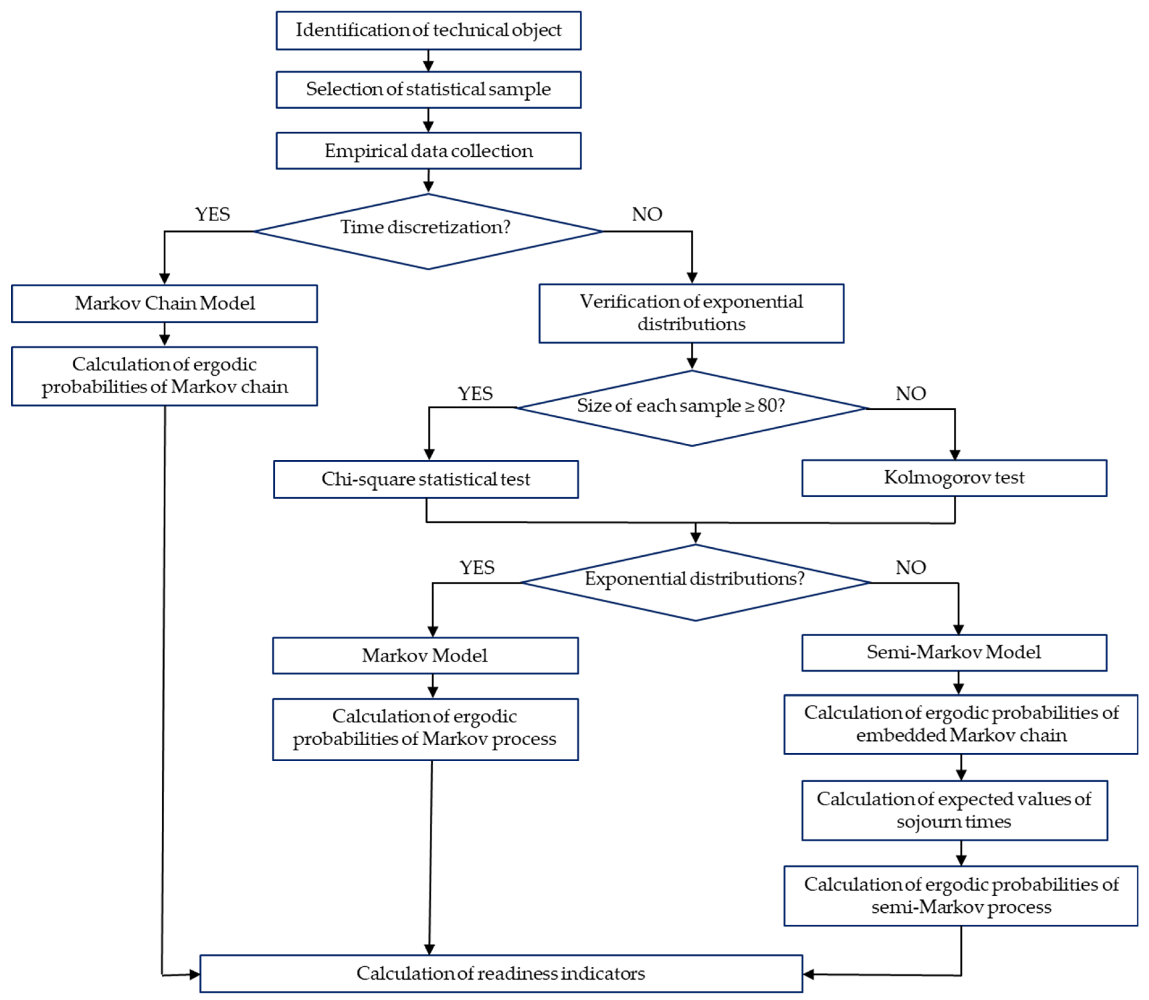
Figure 1 shows a block diagram of creating a model of the exploitation process based on the theory of Markov and semi-Markov. The first stages of stochastic modeling are the identification of the technical object, the selection of a statistical sample, and the collection of empirical data in the form of databases. Then a choice is made between discrete-time and continuous-time models. In the case of discrete-time, a model is constructed based on a Markov chain. When analyzing a process in continuous time, verification of the exponential distribution of time characteristics, a condition for the possibility of using a Markov model, is carried out. Two non-parametric consistency tests are proposed as statistical verification tools: χ² and Kolmogorov, depending on the size of the research samples. For empirical data containing statistical samples less than 80, the Kolmogorov test is recommended, while otherwise, there is no contraindication to using the χ² test [48,49]. For processes satisfying the condition of the exponential distribution, Markov models are used, while otherwise, a semi-Markov model is an appropriate solution. The calculation of the values of operating indicators is carried out on the basis of the ergodic probabilities of the corresponding model.

2.3. Functional Readiness, Technical Efficiency and Technical Suitability

Functional readiness is usually understood as the ability of a technical system or object to undertake and perform tasks consistent with its intended use in the required time [50,51]. The availability index Kr reflects the quantitative characteristic of functional availability, which for the Markov model is expressed as the sum of the probabilities of ergodic operational states k ∈ S_r, in which the object can start the task or is in the process of its implementation. The mathematical notation of this relationship is presented by the formula:

$$K_r={\displaystyle \sum _{k\in S_r}{\pi }_k},$$

(19)

where π_k is the ergodic probability of the desired (from the standpoint of readiness) set of operational states k ∈ S_r.

In functional readiness, the vehicle is technically fully operational, i.e., it has an adequate supply of fuel and consumables and is not being serviced. The functional availability indicator shows the share of time that can be allocated to the implementation of tasks by the technical object during its operation period.

The concept of technical efficiency refers to a wider set of operational states than in the case of functional availability. The technically efficient facility has a technical resource to perform the tasks. However, it may require refueling or short-term maintenance before or after use. For the Markov model, the technical efficiency coefficient K_e is the sum of the ergodic probabilities of operational states l ∈ S_e in which the technical object has a technical service life and does not require periodic maintenance, which is shown in the relationship:

$$K_e={\displaystyle \sum _{l\in S_e}{\pi }_l},$$

(20)

where π_l is the ergodic probability of the desired set of operational states l ∈ S_e.

Technical suitability expresses the condition of a technical object, in which it is not damaged, or there is no need to repair it. The technical suitability condition is an extension of the technical efficiency by the time needed to perform periodic maintenance in order to restore its technical life. The technical suitability index K_s for the Markov model is therefore, the sum of the probabilities of ergodic operational states m ∈ S_s, in which the object is not damaged. This is expressed in the equation:

$$K_s={\displaystyle \sum _{m\in S_s}{\pi }_m},$$

(21)

where π_m is the ergodic probability of the set of operational states m ∈ S_s.

There is the following relationship between the sets defining the states of functional readiness, technical efficiency and technical suitability:

$$S_r\subset S_e\subset S_s.$$

(22)

3. Object of Analysis

3.1. Case Study

The case study of the conducted research is a trial of Honker light utility vehicles, constituting a fleet of vehicles of the military unit transport system. The analyzed technical facilities perform tasks related to the transport of people and small loads weighing up to 1000 kg.

Determining the phase space of the studied process requires the reproduction of a detailed phase trajectory for each object in the three-year research period. In the case of the operation process, one should also take into account the conditions resulting from the operation organization system as well as standards and guidelines for the maintenance subsystem of technical facilities. In the case of military transport systems, the implementation of the vehicle operation process depends on both instructions and procedures developed by the operators of military equipment as part of the adopted operational strategy. As a result of the analysis of the process of light utility vehicles carried out by the authors of this study, a nine-state phase space was identified, for which the possible interstate transitions were specified in

Table 2. State space of the light utility vehicles operation process.

State	Name	Possible Transition from	Possible Transition to
S1	Task execution	S2, S4, S6, S7	S2, S5, S6, S8
S2	Refueling	S1, S3, S4	S1, S3, S5
S3	Parking in garage	S2, S5, S6, S7	S2, S4, S6
S4	Pre-task service	S3	S1, S2
S5	Service after task	S1, S2, S6	S3, S9
S6	Periodic maintenance	S1, S3, S7	S1, S3, S5,
S7	Repair	S8, S9	S1, S3, S6, S9
S8	Diagnostics	S1, S9	S7, S9
S9	Awaiting repair	S5, S7, S8	S7, S8

.

The distinguished operating states are mutually disjoint subsets, which means that at any time t the object may be in only one of them. For example, the vehicle is in the S₃ garage state while waiting to be used. Before starting the task, it is necessary for the direct user to check the correct operation of the systems and mechanisms that determine the safe use of the vehicle. These activities correspond to state S₄. State S₁ means completion of the transportation task, upon completion of which the object should be serviced after use (S₅). Its purpose is to re-check its operational condition, including the removal of minor defects and cleaning the body. The implementation of the S₂ refueling state may occur before, during, or after the task commencement, depending on the identified needs. State S₆ corresponds to the performance of periodic vehicle maintenance in accordance with the operational strategy as well as instructions and guidelines. S₇, S₈ and S₉ states are undesirable from the standby point of view, as they symbolize damage to the object and the need for repair.

The database was developed on the basis of operational documentation covering a three-year research period. Its fragment is presented in

Table 3. Example of a part of database sheet.

No.	Date	Time	S1	S2	S3	S4	S5	S6	S7	S8	S9
267	30.03.2020	08:40:00				1
268	30.03.2020	08:45:00	1
269	30.03.2020	13:31:00		1
270	30.03.2020	13:35:00					1
271	30.03.2020	13:40:00									1
272	31.03.2020	07:00:00								1
273	31.03.2020	07:30:00							1
274	31.03.2020	11:30:00			1
275	04.04.2020	07:20:00				1
276	04.04.2020	07:25:00	1
277	05.04.2020	08:40:00					1
278	05.04.2020	08:45:00			1

. In the following rows of the database, the transitions between the various operational states were identified, along with detailed records in the following system: transition number, date, hour and minute. The accuracy of the measurement in the order of 1 min is determined by the occurrence of short-term states and is necessary to verify the correctness of the time balance over the entire research period.

3.2. Statistical Analysis of Data

For the verification of the empirical distribution with the theoretical distribution, non-parametric consistency tests are commonly used [52,53,54]. The choice of test depends on the type of distribution being verified, the random variable and the sample size. The most common test χ² requires a sample size of at least 80 realizations of a random variable. For a small number of interstate transitions in the operation process, this condition may not be met. In this case, the verification of the assumptions of the Markov process is performed using the Kolmogorov test.

The condition for the exponential distribution of transition times between states was verified with the use of the Kolmogorov conformance test (

Table 4. Results of Kolmogorov test.

Tij	y	Uy Statistics	Critical Range	Hypothesis
T12	798	0.2585	<0.0479, 1>	H1
T15	3340	0.2019	<0.0234, 1>	H1
T16	32	0.1834	<0.2343, 1>	H0
T18	32	0.3587	<0.2343, 1>	H1
T21	396	0.4773	<0.0678, 1>	H1
T23	366	0.4970	<0.0705, 1>	H1
T25	695	0.4731	<0.0513, 1>	H1
T32	365	0.1428	<0.0706, 1>	H1
T34	4063	0.2867	<0.0213, 1>	H1
T36	76	0.2907	<0.1534, 1>	H1
T41	3769	0.6316	<0.0221, 1>	H1
T42	294	0.6151	<0.0786, 1>	H1
T53	3988	0.4533	<0.0215, 1>	H1
T59	70	0.5071	<0.1598, 1>	H1
T61	11	0.4395	<0.3914, 1>	H1
T63	84	0.2843	<0.1461, 1>	H1
T65	23	0.4757	<0.2750, 1>	H1
T71	27	0.2320	<0.2544, 1>	H0
T73	67	0.3295	<0.1632, 1>	H1
T76	10	0.4754	<0.4094, 1>	H1
T79	44	0.4082	<0.2006, 1>	H1
T87	63	0.3348	<0.1683, 1>	H1
T89	39	0.2445	<0.2128, 1>	H1
T97	85	0.2186	<0.1452, 1>	H1
T98	70	0.5196	<0.1598, 1>	H1

). As the H₀ hypothesis, it was assumed that the distribution of T_ij times for individual allowed interstate transitions is consistent with the exponential distribution. The alternative hypothesis (H₁) contradicts this assumption. The U_y statistic of the Kolmogorov test has the form (23):

$$U_y=\underset{1\le i\le y}{max}\left(d_y^{-},d_y^{+}\right),$$

(23)

wherein:

$$d_y^{-}=\underset{1\le i\le y}{max}\left|F\left(x_i\right)-\frac{i-1}{y}\right|,$$

(24)

$$d_y^{+}=\underset{1\le i\le y}{max}\left|\frac{i}{y}-F\left(x_i\right)\right|,$$

(25)

where F(x_i) is the cumulative value of the theoretical distribution according to the H₀ hypothesis, and y is the sample size.

For the U_y statistic values within the range of critical values <D(y;α), 1> for the significance level α, the H₀ hypothesis is rejected and H₁ is accepted. Otherwise, there is no reason to reject the H₀ hypothesis. For the significance level α = 0.05, the value D(y;α) can be approximated using the formula:

$$D\left(0.05;y\right)=\frac{1.358}{\sqrt{y}+0.12+\frac{0.11}{\sqrt{y}}}.$$

(26)

At the adopted significance level of α = 0.05, only two time characteristics, T₁₆ and T₇₁, achieved the values of the Kolmogorov test statistics, which are not included in the critical intervals. This means there are no grounds to reject the null hypothesis assuming the exponential distribution of the times of stay in individual states. Thus, for the remaining time characteristics, the null hypothesis was rejected and an alternative was adopted. The results of the statistical test for all variables are presented in Table 4. Figure 2 presents the frequency graphs for two exemplary times T₁₆ and T₃₄ and the course of the exponential distribution with the parameter estimated on the basis of the reciprocal of the mean values from both statistical samples. The number of histogram intervals was determined using the square root method.

The exploitation process does not fulfill the condition of exponential distributions and, therefore, cannot be considered a Markov process in continuous time. In this case, semi-Markov processes should be used for modeling.

4. Results and Discussions

4.1. Semi-Markov Model (SMM)

The embedded Markov chain in the semi-Markov process, in accordance with the adopted assumptions, does not allow for the possibility of returns (transition from the S_i state to the S_i state). This assumption adopts that every change of the process state is recorded, while its absence means that the object is in the S_i state before transitioning to the next S_j state for a period of time equal to T_ij [26,28,29,30]. The matrix (27) shows the empirical numbers of transitions between particular exploitation states as a result of observation of the process. On the other hand, matrix (28) represents the probabilities of transitions between states estimated on the basis of the matrix of the number of transitions.

$$N=\left[\begin{array}{ccccccccc}0& 798& 0& 0& 3340& 32& 0& 32& 0\\ 396& 0& 366& 0& 695& 0& 0& 0& 0\\ 0& 365& 0& 4063& 0& 76& 0& 0& 0\\ 3769& 294& 0& 0& 0& 0& 0& 0& 0\\ 0& 0& 3988& 0& 0& 0& 0& 0& 70\\ 11& 0& 84& 0& 23& 0& 0& 0& 0\\ 27& 0& 67& 0& 0& 10& 0& 0& 44\\ 0& 0& 0& 0& 0& 0& 63& 0& 39\\ 0& 0& 0& 0& 0& 0& 85& 70& 0\end{array}\right],$$

(27)

$$P=\left[\begin{array}{ccccccccc}0& 0.189910& 0& 0& 0.794860& 0.007615& 0& 0.007615& 0\\ 0.271791& 0& 0.251201& 0& 0.477008& 0& 0& 0& 0\\ 0& 0.081039& 0& 0.902087& 0& 0.016874& 0& 0& 0\\ 0.927640& 0.072360& 0& 0& 0& 0& 0& 0& 0\\ 0& 0& 0.982750& 0& 0& 0& 0& 0& 0.017250\\ 0.093220& 0& 0.711864& 0& 0.194915& 0& 0& 0& 0\\ 0.182432& 0& 0.452703& 0& 0& 0.067568& 0& 0& 0.297297\\ 0& 0& 0& 0& 0& 0& 0.617647& 0& 0.382353\\ 0& 0& 0& 0& 0& 0& 0.548387& 0.451613& 0\end{array}\right].$$

(28)

Table 5. Standard errors of probabilities estimation.

SE(pij)	S1	S2	S3	S4	S5	S6	S7	S8	S9
S1	0	0.0061	0	0	0.0062	0.0013	0	0.0013	0
S2	0.0117	0	0.0114	0	0.0131	0	0	0	0
S3	0	0.0041	0	0.0044	0	0.0019	0	0	0
S4	0.0041	0.0041	0	0	0	0	0	0	0
S5	0	0	0.0020	0	0	0	0	0	0.0020
S6	0.0268	0	0.0417	0	0.0365	0	0	0	0
S7	0.0317	0	0.0409	0	0	0.0206	0	0	0.0376
S8	0	0	0	0	0	0	0.0481	0	0.0481
S9	0	0	0	0	0	0	0.0400	0.0400	0

summarizes the values of the standard error for the conditional probabilities (28) estimated on the basis of the matrix of the number of interstate transitions (27). According to Formula (6), with the increase in the number of transitions from the S_i state, the standard error SE(p_ij) decreases. For this reason, the values of the standard error are higher for operational states in which the technical object is relatively rare. Nevertheless, for all conditional probabilities, the SE(p_ij) did not exceed the value of 0.05 [55,56]. The result at this level is considered acceptable.

Figure 3 presents a graph illustrating possible transitions between states during the implementation of the operation process. According to the assumptions made for the embedded Markov chain, the fact that the object remains in the same state is not treated as a S_i → S_i transition. For this reason, the SMM model graph does not have connections coming from the S_i state and going directly to the S_i state. This means a lack of return to the same state, which is commonly used in modeling the operation processes.

Assuming that at t = 0, the vehicle is technically efficient and awaits the appearance of the task, it is possible to determine the instantaneous probabilities of the embedded Markov chain. This assumption reflects the initiation of the operation process for a vehicle included in the transport system. The instantaneous probabilities are the matrix product of the initial distribution matrix p₀ and the n-th power of the conditional probability matrix P, where n corresponds to the number of transitions between states. The development of the dependence of the instantaneous probabilities on the number of interstate transitions allows us to determine the period after which their values stabilize at a certain level and the stochastic process reaches the equilibrium state.

Figure 4 and Figure 5 show changes in the value of the instantaneous probabilities of the embedded Markov chain in the semi-Markov process. In the range from t = 0 to t = 30, there are fluctuations with a large amplitude of changes in the values, which decrease with time and after overcoming about 50 transitions, the probability values remain constant.

4.2. Ergodic Probabilities of SMM

The ergodic probabilities of the semi-Markov process are determined on the basis of the probabilities of the embedded Markov chain and the values of the expected time in individual states of the process. For the embedded Markov chain, the ergodic probabilities are computed using the matrix equation:

$$(P^T-I)\cdot P_j=\left[\begin{array}{ccccccccc}-1& p_{21}& 0& p_{41}& 0& p_{61}& p_{71}& 0& 0\\ p_{12}& -1& p_{32}& p_{42}& 0& 0& 0& 0& 0\\ 0& p_{23}& -1& 0& p_{53}& p_{63}& p_{73}& 0& 0\\ 0& 0& p_{34}& -1& 0& 0& 0& 0& 0\\ p_{15}& p_{25}& 0& 0& -1& p_{65}& 0& 0& 0\\ p_{16}& 0& p_{36}& 0& 0& -1& p_{76}& 0& 0\\ 0& 0& 0& 0& 0& 0& -1& p_{87}& p_{97}\\ p_{18}& 0& 0& 0& 0& 0& 0& -1& p_{98}\\ 0& 0& 0& 0& p_{59}& 0& p_{79}& p_{89}& -1\end{array}\right]\cdot \left[\begin{array}{c}{p}_1\\ p_2\\ p_3\\ p_4\\ p_5\\ p_6\\ p_7\\ p_8\\ p_9\end{array}\right]=\left[\begin{array}{c}0\\ 0\\ 0\\ 0\\ 0\\ 0\\ 0\\ 0\\ 0\end{array}\right],$$

(29)

which can be written as a system of Equation (30) together with the condition (31) of system normalization:

$$\{\begin{array}{c}-p_1+0.271791p_2+0.927640p_4+0.093220p_6+0.182432p_7=0\\ 0.189910p_1-p_2+0.081039p_3+0.072360p_4=0\\ 0.251201p_2-p_3+0.982750p_5+0.711864p_6+0.452703p_7=0\\ 0.902087p_3-p_4=0\\ 0.794860p_1+0.477008p_2-p_5+0.194915p_6=0\\ 0.007615p_1+0.016874p_3-p_6+0.067568p_7=0\\ -p_7+0.617647p_8+0.548387p_9=0\\ 0.007615p_1-p_8+0.451613p_9=0\\ 0.017250p_5+0.297297p_7+0.382353p_8-p_9=0\end{array},$$

(30)

$${\displaystyle \sum _{j=1}^9{p}_j}=1.$$

(31)

After solving the system of equations, the values of ergodic probabilities p_j of the inserted Markov chain were obtained. The expected E(T_j) times of staying in individual operating states were determined as average values based on empirical data. The values of p_j and E(T_j) were used to calculate the values of ergodic probabilities in the semi-Markov model. The results of the conducted analyses are summarized in

Table 6. Ergodic probabilities of states in embedded Markov chain and SMM.

State	S1	S2	S3	S4	S5	S6	S7	S8	S9
pj	0.223537	0.077505	0.239575	0.216117	0.215872	0.006267	0.007722	0.005343	0.008063
E(Tj) (min)	717.52	4.60	3956.58	5.00	8.13	271.95	174.63	36.11	13,240.50
πj	0.131311	0.000292	0.776024	0.000885	0.001436	0.001395	0.001104	0.000158	0.087396
πj (%)	13.1311	0.0292	77.6024	0.0885	0.1436	0.1395	0.1104	0.0158	8.7396

.

The garage state S₃ had the highest value of the ergodic probability of over 77%. On the basis of the calculated values of probabilities, it can be concluded that the trucks and passenger cars stay together in other states for approximately 13% of the time during the entire three-year research period. The S₉ state also obtained a significant level of ergodic probability, which indicates that the vehicles remain in a state of waiting for repair for almost 9% of their operational time. The remaining operational states obtained probability values below 1% and do not have a significant impact on the availability rates.

4.3. Calculations of Indicators in SMM

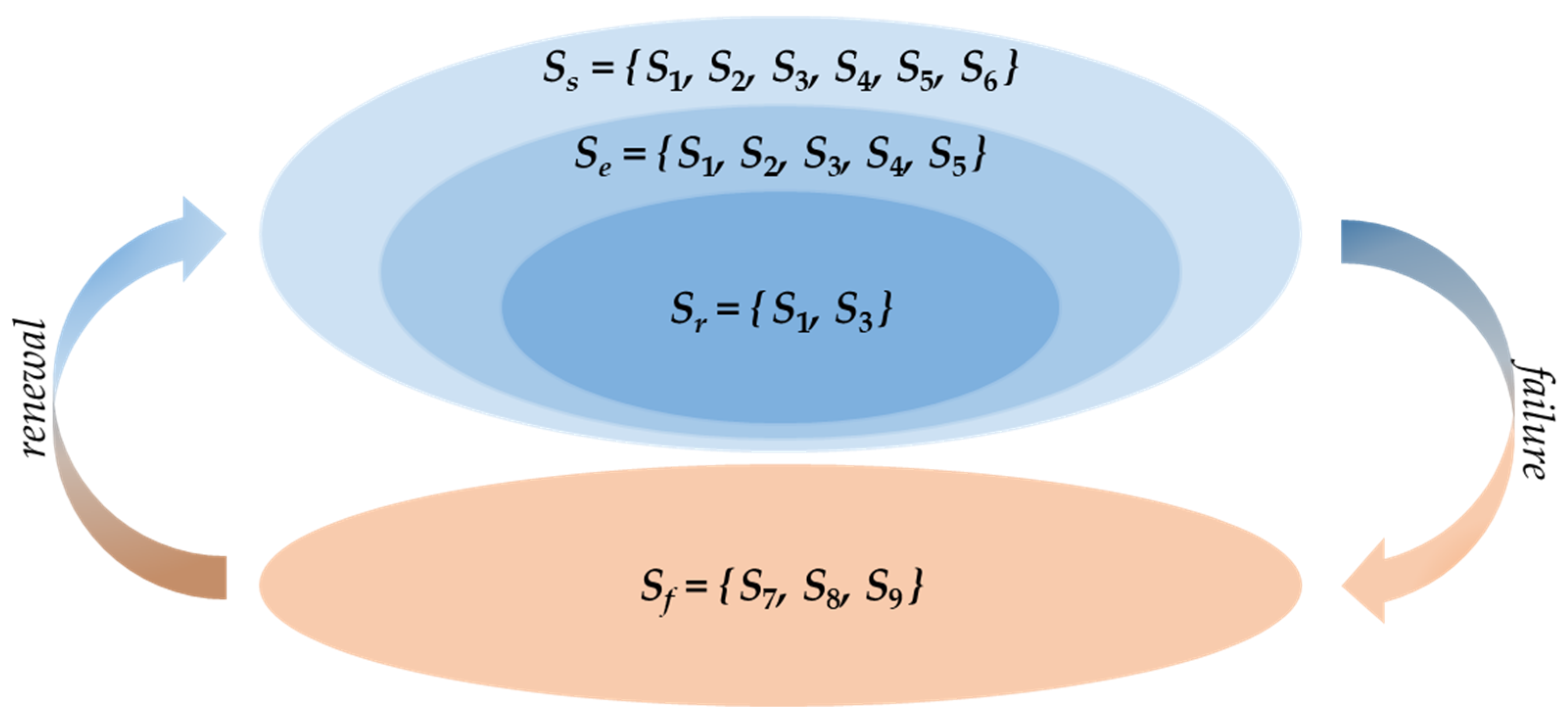
In the nine-state exploitation model, state subsets were distinguished corresponding to the functional readiness S_r, technical efficiency S_e and technical suitability S_s. The mathematical notation is presented by the Formulas (32)–(34):

$$S_r=\left\{S_1,S_3\right\},$$

(32)

$$S_e=\left\{S_1,S_2,S_3,S_4,S_5\right\},$$

(33)

$$S_s=\left\{S_1,S_2,S_3,S_4,S_5,S_6\right\}.$$

(34)

Functional readiness corresponds to the vehicle being in the task (S₁) or garage (S₃) state. Technical efficiency extends the set of these states with fuel refilling (S₂) and the implementation of maintenance before starting the task (S₄) and after its completion (S₅). On the other hand, technical suitability also takes into account the implementation of periodic maintenance (S₆), the purpose of which is to restore the technical service life. The graphical diagram of the division of the operating conditions set into individual subsets is shown in Figure 6.

For such defined subsets, the values of functional availability, technical efficiency and technical suitability indicators were calculated. The results are presented in

Table 7. Values of K_r, K_e and K_s indicators in SMM.

Indicator	Value
Functional readiness Kr	0.907334
Technical efficiency Ke	0.909947
Technical suitability Ks	0.911343

. The values of all three indicators are similar, which means a small share of the time of current and periodic maintenance and refueling in the entire test period.

The high probability value of the S₉ ergodic state has the greatest impact on the reduction of the indicators of functional availability, technical efficiency and technical suitability of vehicles. This state corresponds to the situation when the vehicle has suffered a breakdown, is out of order and requires repair. Due to the lack of technical possibilities, it is not in the repair state (S₇) and is not in the diagnosis phase (S₈). The main reasons for such a situation are logistic delays related to the limited availability of spare parts and the lack of qualified technical personnel within the specified time.

4.4. Sensitivity Analysis of SMM

The calculated ergodic probability π₉ of the S₉ state has the strongest impact on the values of the K_r, K_e and K_s indicators. Due to this fact, the sensitivity analysis of the SMM model was carried out in order to investigate the impact of the presence of objects in the S₉ state on the ergodic probabilities and technical readiness rates. The parameter against which the variability analysis was performed is the expected value of the duration of the S₉ state. For the change of this parameter, expressed as a percentage and amounting to ΔE(T₉), the values of the ergodic probabilities of the semi-Markov process can be determined using the relationship:

$${\pi }_j=\frac{p_j\cdot E\left(T_j\right)}{{\displaystyle {\sum }_{i=1}^8{p}_i\cdot E\left(T_i\right)+p_9\cdot E\left(T_9\right)\cdot \left(1-\Delta E\left(T_9\right)\right)}} \mathrm{for} j=\left\{1,2,3,\dots ,8\right\},$$

(35)

$${\pi }_9=\frac{p_9\cdot E\left(T_9\right)\cdot \left(1-\Delta E\left(T_9\right)\right)}{{\displaystyle {\sum }_{i=1}^8{p}_i\cdot E\left(T_i\right)+p_9\cdot E\left(T_9\right)\cdot \left(1-\Delta E\left(T_9\right)\right)}}.$$

(36)

The undoubted advantage of the SMM model is the ability to perform a sensitivity analysis for a wide range of changes in the E(T₉) parameter without the need to solve many matrix equations.

Table 8. Ergodic probabilities obtained in sensitivity analysis of SMM.

ΔE(T9) (%)	π1	π2	π3	π4	π5	π6	π7	π8	π9
0	0.131311	0.000292	0.776024	0.000885	0.001436	0.001395	0.001104	0.000158	0.087396
10	0.132468	0.000294	0.782865	0.000893	0.001449	0.001407	0.001114	0.000159	0.079350
20	0.133646	0.000297	0.789828	0.000901	0.001462	0.001420	0.001124	0.000161	0.071162
30	0.134846	0.000300	0.796916	0.000909	0.001475	0.001433	0.001134	0.000162	0.062826
40	0.136067	0.000302	0.804133	0.000917	0.001488	0.001446	0.001144	0.000164	0.054339
50	0.137310	0.000305	0.811481	0.000926	0.001502	0.001459	0.001154	0.000165	0.045698
60	0.138577	0.000308	0.818965	0.000934	0.001515	0.001472	0.001165	0.000167	0.036897
70	0.139867	0.000311	0.826588	0.000943	0.001530	0.001486	0.001176	0.000168	0.027932
80	0.141181	0.000314	0.834354	0.000952	0.001544	0.001500	0.001187	0.000170	0.018799
90	0.142520	0.000317	0.842268	0.000961	0.001559	0.001514	0.001198	0.000171	0.009492

shows the results of the analysis for selected ΔE(T₉) values. Figure 7 presents a graph of changes in ergodic probabilities for continuous changes in the value of ΔE(T₉).

On the basis of the determined ergodic probabilities, the possibilities of improving the values of the readiness ratios were carried out at the assumed levels of reduction of the time spent in the state of incapacity and waiting for repair. The results are presented in

Table 9. Indicators values obtained in sensitivity analysis of SMM.

ΔE(T9) (%)	Kr	ΔKr	Ke	ΔKe	Ks	ΔKs
0	0.907334	0.000000	0.909947	0.000000	0.911343	0.000000
10	0.915334	0.008000	0.917970	0.008023	0.919377	0.008035
20	0.923476	0.016142	0.926135	0.016188	0.927555	0.016213
30	0.931764	0.024430	0.934447	0.024500	0.935880	0.024538
40	0.940202	0.032868	0.942910	0.032962	0.944356	0.033013
50	0.948794	0.041460	0.951527	0.041580	0.952986	0.041643
60	0.957545	0.050211	0.960303	0.050356	0.961775	0.050433
70	0.966459	0.059125	0.969243	0.059295	0.970729	0.059386
80	0.975541	0.068206	0.978350	0.068403	0.979850	0.068508
90	0.984794	0.077460	0.987630	0.077683	0.989145	0.077802

and Figure 8.

Reducing the waiting time for repairs by 50% would result in an increase in the values of the K_r, K_e and K_s indicators to the level of about 0.95, which at the same time means their improvement by over 0.04. The sensitivity analysis of the SMM model was carried out with regard to the impact of changes in the expected value of the time of staying in the S₉ state.

4.5. Markov Model (MM)

Markov models, assuming exponential distributions of time characteristics, often use stochastic models to describe the operation processes of machines, devices and technical systems. For small deviations of empirical distributions of interstate times from the theoretical assumptions of the Markov theory, the results obtained for Markov and semi-Markov models may be similar or even negligibly small.

For the analyzed sample of means of transport, the non-parametric Kolmogorov test showed grounds for rejecting the null hypothesis about exponential distributions. However, the authors of the publication conducted an analysis of the applicability of the Markov model as a simplification of the generalized SMM presented in Section 4.1, Section 4.2, Section 4.3 and Section 4.4. The basic characteristic of the Markov model is the matrix of interstate transition intensity Λ. In the case study under consideration, the value of the Λ matrix presented in the matrix, which were estimated on the basis of the mean values of the transition times between the states according to the Equations (11) and (12).

$$\Lambda =\left[\begin{array}{ccccccccc}-0.012136& 0.000890& 0& 0& 0.001593& 0.007880& 0& 0.001773& 0\\ 0.214402& -0.657021& 0.229036& 0& 0.213583& 0& 0& 0& 0\\ 0& 0.000241& -0.000650& 0.000257& 0& 0.000152& 0& 0& 0\\ 0.199841& 0.200000& 0& -0.399841& 0& 0& 0& 0& 0\\ 0& 0& 0.122711& 0& -0.270079& 0& 0& 0& 0.147368\\ 0.003216& 0& 0.003819& 0& 0.003446& -0.010481& 0& 0& 0\\ 0.007004& 0& 0.005194& 0& 0& 0.010753& -0.028343& 0& 0.005392\\ 0& 0& 0& 0& 0& 0& 0.045652& -0.062586& 0.016934\\ 0& 0& 0& 0& 0& 0& 0.000068& 0.000088& -0.000156\end{array}\right].$$

(37)

Ergodic probabilities of the Markov process for the entire set of operational states are calculated by solving the matrix Equation (38) together with the system normalization condition (39).

$${\Pi }^T\cdot \Lambda ={\left[\begin{array}{c}{\pi }_1\\ {\pi }_2\\ {\pi }_3\\ {\pi }_4\\ {\pi }_5\\ {\pi }_6\\ {\pi }_7\\ {\pi }_8\\ {\pi }_9\end{array}\right]}^T\cdot \left[\begin{array}{ccccccccc}-{\lambda }_{11}& {\lambda }_{21}& 0& {\lambda }_{41}& 0& {\lambda }_{61}& {\lambda }_{71}& 0& 0\\ {\lambda }_{12}& -{\lambda }_{22}& {\lambda }_{32}& {\lambda }_{42}& 0& 0& 0& 0& 0\\ 0& {\lambda }_{23}& -{\lambda }_{33}& 0& {\lambda }_{53}& {\lambda }_{63}& {\lambda }_{73}& 0& 0\\ 0& 0& {\lambda }_{34}& -{\lambda }_{44}& 0& 0& 0& 0& 0\\ {\lambda }_{15}& {\lambda }_{25}& 0& 0& -{\lambda }_{55}& {\lambda }_{65}& 0& 0& 0\\ {\lambda }_{16}& 0& {\lambda }_{36}& 0& 0& -{\lambda }_{66}& {\lambda }_{76}& 0& 0\\ 0& 0& 0& 0& 0& 0& -{\lambda }_{77}& {\lambda }_{87}& {\lambda }_{97}\\ {\lambda }_{18}& 0& 0& 0& 0& 0& 0& -{\lambda }_{88}& {\lambda }_{98}\\ 0& 0& 0& 0& {\lambda }_{59}& 0& {\lambda }_{79}& {\lambda }_{89}& -{\lambda }_{99}\end{array}\right]={\left[\begin{array}{c}0\\ 0\\ 0\\ 0\\ 0\\ 0\\ 0\\ 0\\ 0\end{array}\right]}^T,$$

(38)

$${\displaystyle \sum _{j=1}^9{\pi }_j}=1.$$

(39)

Mathematica and MS Excel software were used for the presented calculations. The results for MM are summarized in

Table 10. Comparison of results obtained by MM and SMM.

	π1	π2	π3	π4	π5	π6	π7	π8	π9
SMM	0.131311	0.000292	0.776024	0.000885	0.001436	0.001395	0.001104	0.000158	0.087396
MM	0.012784	0.000172	0.275931	0.000177	0.000435	0.017489	0.003780	0.001325	0.687906
difference	−0.118527	−0.000120	−0.500093	−0.000708	−0.001001	0.016094	0.002676	0.001167	0.600510
difference in %	−90.26	−41.10	−64.44	−80.00	−69.71	1153.69	242.39	738.61	687.11

and Figure 9, comparing them with the values of ergodic probabilities obtained for SMM. Percentage differences between the models reached significant values, with the most similar probabilities occurring for the S₂ state and differing by over 41.0%. The greatest discrepancies in the results occurred for the S₆ state, for which the ergodic probability obtained in MM was as much as 1153.69% higher than in SMM. In addition, the S₆, S₇, S₈ and S₉ states, which are a subset of the technical inoperability and failure states, achieved positive differences. The use of MM to evaluate the operation process would result in a significant reduction of the values of the K_r, K_e, and K_s indices, inconsistent with the actual state.

Compared to SMM, the Markov model achieved a mean absolute percentage error (MAPE) of 351.92%. Therefore, the hypothesis about the possibility of using the Markov process to describe state changes by the analyzed technical objects in the considered nine-element set of operational states should be unambiguously rejected.

5. Conclusions

The theory of Markov processes was used to model the operation of light utility vehicles. The paper presents a semi-Markov model that allows for the assessment the technical readiness of means of transport operating in a real system. On the basis of the systems of Chapman–Kolmogorov equations and the values of the expected times of stay in operating states, the values of the ergodic probabilities of the process were determined. The main reason for the reduction of functional availability, technical efficiency and technical suitability indicators was the high probability value of the S₉ state (Awaiting repair). This indicates the occurrence of significant delays in the implementation of repairs of damaged vehicles. Therefore, in eliminating the reasons for the presence of technical objects in the S₉ state, the operating system does not have sufficient technical resources to carry out repairs without unnecessary time delay. Repair delays are mainly caused by the unavailability of spare parts and a shortage of qualified technical personnel. In order to maximize the technical readiness of vehicles, it is necessary to focus on improving the organization of the spare parts delivery system, which will significantly reduce the time spent by technical facilities in the S₉ state.

For the current state of the operation system, the functional availability ratio K_r has reached the value of 0.907334, which should be interpreted as follows: for more than 90% of the duration of the operation process, vehicles in good technical condition await the appearance of a task or are in the process of its implementation. A slight difference between the technical efficiency index K_e and the functional readiness index K_r indicates that the process of refueling and servicing is carried out efficiently. The aforementioned processes constitute a set of activities preparing a technically efficient vehicle to perform the task, as well as control and check after its completion. On the other hand, the technical suitability index K_s amounting to 0.911343 means that for over 91% of the duration of the operation process, the vehicles are fit for use. Its high value indicates a well-thought-out and proper implementation of the exploitation strategy. The small value of the ergodic probability for the S₆ state resulted in a slight difference between the technical efficiency index K_e and the technical suitability index K_s. The above-mentioned results show that the capabilities of the technical subsystem, which carries out the periodic maintenance process, are adjusted to the requirements of the plan-preventive strategy used.

The ergodic probability π₂ of 0.000292 and the expected residence time in the S₂ state of 4.60 (min) indicate an efficiently implemented refueling process. For the current level of intensity of use of vehicles, in which over 13.0% of the operation time is during the implementation of transport tasks, the technical system provides sufficient resources of diesel oil and appropriate distribution equipment.

Despite the assumed high level of readiness, efficiency and suitability indicators of the tested military vehicles, an attempt was made to optimize the process by determining the impact of a potential reduction in the duration of the S₉ state, equipped with logistic delays occurring in the operation system. An analysis of the optimization possibilities was carried out on the basis of changes in the expected time of stay in the S₉ state based on analytical relationships, which enabled the analysis based on a continuous reduction of changes in E(T₉) in the percentage range of 0.0–90.0%. As a result, the reduction of the expected time of the vehicle’s stay in the S₉ state by 50.0% resulted in the increase of all indicators by over 0.041, and the reduction by 90% increased the values of the indicators by over 0.077.

The attempt to use the Markov process, despite not meeting the condition of exponential time characteristics, showed significant discrepancies between MM and SMM. The high degree of mismatch between the Markov model and the actual process is evidenced by the value of the MAPE error amounting to 351.92%. Therefore, it is inappropriate to use MM to describe the nine-state process of operation of heavy goods vehicles operating in the military transport system. The performed non-parametric Kolmogorov test resulted in the rejection of the hypothesis concerning the compatibility of empirical distributions of the duration of individual states with the theoretical exponential distribution.

The proposed method allows a detailed analysis of vehicle operation as a stochastic process with a multi-state phase space. The unquestionable advantage of the nine-state semi-Markov model is the possibility of evaluating the operation process using indicators of functional readiness, efficiency, and technical efficiency, calculated based on the basis of ergodic probabilities of the process. Additionally, the model sensitivity analysis makes it possible to determine the impact of reducing the values of expected vehicle dwell times in each state on the efficiency of the operation process. However, a disadvantage of the proposed method is the inability to predict the values of indicators for the increased or decreased intensity of vehicle use expressed by means of average daily mileage. This is due to the condition of determining the characteristics of all states in the same time domain.

The proposed methodology for creating stochastic exploitation models can be applied to a wide range of facilities and technical devices. The developed model can be used to analyze and evaluate the operation process of other vehicles operating in technical systems with an analogous or similar operation strategy.