Conditional Dynamic Dependence and Risk Spillover between Crude Oil Prices and Foreign Exchange Rates: New Evidence from a Dynamic Factor Copula Model

Abstract

This paper proposes a dynamic factor model to accurately characterize the dynamic dependence and risk spillovers between the crude oil and exchange rate returns of oil-trading countries from 2000–2020, conditional on the common factors. To this end, we first identify the common factors related to returns of crude oil prices and exchange rates from 14 typical oil-trading countries. Then, we use the AR-GARCH model to filter the respective idiosyncratic factors and conduct a comparative study of conditional dynamic dependence between the crude oil and exchange rate returns of oil importers and exporters. Finally, we combine the dynamic factor copula model with the CoVaR method to measure the conditional risk spillover effect between crude oil and exchange rate markets. The empirical study indicates that the classical factor analysis can be used to precisely identify the common factors related to both financial markets, with the similar trend of macro-economic indicators. Furthermore, the factor copula model can capture the dynamic structure between crude oil and exchange rate markets more accurately than the traditional Copula–GARCH model. Specifically, the idiosyncratic factors related to each return series still have a significant impact on the dependence between the crude oil and exchange rate returns of oil importers, while the common factors have played an important role in the relationship of oil exporters’ exchange rates with crude oil prices. Finally, the crude oil market has enjoyed a relative risk premium to the exchange rate markets of oil-trading countries. However, there is almost no conditional risk spillover from the corresponding exchange rates to the crude oil prices. Finally, we discuss the implications for investors, policymakers and respective exchange rate regulators from oil-trading countries with further insights from the macro-economic perspective.

1. Introduction

Since international crude oil trades are settled in United States dollars, the crude oil supply and demand shocks can affect international oil prices and further change the supply–demand relationship of the international exchange rate markets. It ultimately results in the fluctuation of the exchange rate markets of the respective oil-trading countries. Therefore, the volatility of the crude oil market has an important connection with the financial markets and macroeconomics of oil-trading countries. Then, the researchers have identified the closer link between oil prices and the exchange rates of major OPEC member countries in both short and long terms [1,2]. Particularly, the respective exchange market regulators have paid more attention to the increasing prominent risk spillover effect between the crude oil market and the exchange rate market.

It is generally believed that a devaluation of the dollar can increase the purchasing power and then raise the other importers’ demand for crude oil, which then contributes to the rise of crude oil prices. Nevertheless, there is still no consensus over how the increase of crude oil prices affects the USD’s exchange rate [3]. The higher oil price can lead to the reduction in both production and trade from the U.S., giving rise to the depreciation of the USD. However, the increase in crude oil price can also have a negative impact on the trade of other oil importers, i.e., Japan and the European Union, leading to the depreciation of the JPY and EUR but the appreciation of the USD. Therefore, there is a direct connection between crude oil price and the real exchange rate of the USD relative to other currencies because the USD has been considered as the major invoicing and settlement currency. To this end, it is crucial for the respective investors and market regulators from oil-trading countries to conduct robust modeling for their dependence in order to improve respective investment decision making and portfolio risk management.

Dependence models based on copula functions offer an elegant approach for modeling multivariate distributions in many research fields, especially about the dependence structure among the financial markets. Compared with traditional approaches, such as the multivariate GARCH or SV models, the copula model can be used to build flexible joint distributions of the financial asset returns rather than the idealized multivariate normal distribution. A number of parametric copula models therefore can be adopted to capture the tail and asymmetric dependence structure presented in the financial time series. This approach can allow the various marginal distributions without normality restrictions and incorporates more accurate information into the joint distribution [4]. Therefore, we try to use this method to characterize the time-varying dependence structure between the crude oil market and the foreign exchange market.

Furthermore, this paper has tried to construct a dynamic factor copula model to study the dependence structure among the crude oil and exchange rate returns of oil-trading countries. As we know, the joint distribution function of financial variables in large dimensions is difficult to determine due to the stochastic nature of the market and the diversity of financial assets [5]. However, Granger et al. [6] emphasized that the so-called dominant common factors generally determine the major time-series properties of two or just a few series. These common factors may be either directly observed or derived from other series in the system, as in simple cointegration. With this situation in mind, we can first identify the common factors affecting both oil and exchange rate markets, which have not been paid attention by the relevant research about the vine copula model. Then we can use the factor copula model to more precisely capture the conditional dynamic dependences among the financial markets by extracting their common factors.

We also conduct a comparative study of conditional dynamic dependence between crude oil and exchange rate returns of oil-trading countries in the empirical study. The exchange rate of the USD can influence the real economy of oil-trading countries through oil price shocks. Specifically, the relatively weak USD may increase the purchasing power of oil importers but decrease the purchasing power of oil exporters [7]. Then, if the crude oil price rises, the respective wealth will be transferred from oil-importing countries to oil-exporting countries [8]. Therefore, there are differences in the relationship of the crude oil price with the exchange rate of oil exporters and oil importers. For example, Yang et al. [9] and Reboredo [10] argued that the link magnitude is larger for oil-exporting countries. Furthermore, the sign of the relationship can be negative for oil-exporting countries but mixed for oil-importing countries [11,12]. Therefore, the research on the comparison of the dependence structure between crude oil and exchange rate returns has crucial implications for the investors and financial market regulators from oil-trading countries.

The identified dynamic dependence between financial markets can be used to examine the trends in long-term links among the crude oil returns and exchange rate returns of oil importers and exporters, respectively. Therefore, it is necessary for us to further explain how the two interact with each other in terms of risk dependence. Then we try to measure the conditional risk spillover from extreme perspectives based on the factor copula model as well. Risk spillover refers to the transmission of risk from one market (industry or institution) to another market (industry or institution). At the given confidence level, the conditional value at risk (CoVaR) can be used to portray the maximum potential loss of other assets for a certain holding period when the loss of a given asset is VaR at a specific time in the future [13]. Then we can use the empirical results from the factor copula model to evaluate the risk spillover between crude oil returns and foreign exchange rate returns of oil trading countries.

Therefore, we try to propose a dynamic factor copula model to characterize the conditional dynamic dependence structure and risk spillover effect between crude oil and exchange rate returns of oil-trading countries. Then this paper can contribute to the previous literature in the following ways. First, we utilize the factor copula model to analyze the non-linear dependence structure between crude oil and exchange rate markets. Conditional on the common factors affecting both markets, the approach can be proposed to characterize the interdependence between crude oil returns and exchange rate returns more accurately than the tradition Copula–GARCH model. Second, we propose a comparative study for the dynamic dependence structure between the crude oil returns and exchange rate returns from oil importers and exporters, respectively. It may be the first time to calculate the respective dynamic conditional dependence by employing five representative time-varying factor copula models. Last but not the least, we combine the dynamic factor copula model with the CoVaR method to measure the risk spillover effect between crude oil and exchange rate markets. The analysis of the extreme movement of exchange rates conditional on the extreme risk of crude oil returns can provide strong evidence for respective potential risk spillover from the crude oil to exchange rate markets.

Our corresponding empirical findings have important implications for risk management, especially in the exchange rate regulations of oil-trading countries. The respective financial investors and market risk managers can use this approach to identify the common factors related to the risk among these financial markets. As a closer adherence to reality, the empirical study from the factor copula model can provide them more accurate results about the risk co-movement between crude oil prices and exchange rates from oil-trading countries from the perspectives of extreme market risks. Therefore, our study can guide financial investors to adapt their oil-exchange-rate portfolio strategy in order to deal with the extreme risks in the respective financial markets. Furthermore, we can help the financial regulators from oil-trading countries to strengthen the regulatory policy for their exchange rates in order to resist risk spillovers from the oil market.

The remainder of the paper is structured as follows. Relevant literature is presented in Section 2. Section 3 introduces the dynamic factor copula model and risk spillover measuring model. Section 4 presents the data and summary statistics. Empirical results are showed in Section 5. Finally, Section 6 concludes the paper.

2. Literature Review

With the increase in the degree of financial market openness, a lot of approaches have been used to measure their dependence structure. As the simplest and widely used method, the calculation of linear correlation coefficient needs to assume that the marginal distribution has a Gaussian distribution. However, the financial returns typically display the unfair distribution, heavy tail and some degree of skewness [14]. Therefore, the copula model, a flexible approach has been generally considered as a powerful tool to capture a more realistic dependence structure across markets. We can use this approach to well describe the nonlinear and tail dependence structures, without any constraints on the marginal distributions of random variables [15]. Especially, it is efficient to adopt this approach to characterize the extreme co-movement between the financial markets under risk situations. Thus, the copula models have been widely used in the field of market contagion and risk spillover.

An important innovation in the copula literature has been the availability of parametric models in higher dimensional settings. At this moment, classical Gaussian and Student copula models are still rather restrictive. Then the class of vine copulas has been proposed to solve high-dimensional problems. In contrast with vine copulas, Krupskii and Joe [16] and Oh and Patton [17] introduced the so-called factor copula models to characterize the time-series dependence in high dimensions. In contrast to the traditional factor models, factor copulas have paid more attention to the copula structure implied by a latent factor model rather than their marginal information. Therefore, this approach can be used to capture the dependence structure by a low number of parameters in relatively high-dimensional applications [18].

As typical financial markets, the dependence structure between crude oil and foreign exchange rate markets has received more attention from researchers and market regulators in the oil-trading countries. They have identified a long-term dynamic dependence and mutual effect between the crude oil and exchange rate markets (Beckmann et al. [2], Nikbakh [1]). Furthermore, Huang et al. [7] and Lin and Su [19] discussed the heterogeneity in the dynamic response of exchange rates in oil-trading countries to the crude oil price shocks. In addition, most of the relevant literature focuses on the respective interdependence across the markets [20,21,22,23]. Nevertheless, the economically adequate approach has failed to consider the common factors related to these markets. Then, it is necessary to further study the interdependence among the financial markets more accurately.

To our knowledge, the so-called common factors may come from several types of indicators in connection with the overall economic environment: for instance, the indicators related to the investors’ economic expectation including the global consumer information index, oil price volatility index (OVX) and the indicators related to the economic and financial health of relevant listed companies such as the stock price index or stock market shock [24,25]. Taking the global consumer information index as an example, the COVID-19 pandemic has caused consumers to engage in panic buying of storable consumer goods. This then leads to the volatility in prices of raw materials, such as crude oil, as well as the exchange rates of both their exporters and importers. Furthermore, common factors may include some exogenous variables that are not easily measured such as the political environment or the financial policy. These factors can affect the volatility of an individual market as well as the overall interdependence between crude oil markets and exchange rate markets directly and indirectly. It would therefore be useful to precisely capture the risk interdependence among markets conditioned on common factors.

The concept of the factor copula model was firstly proposed by Ledoit and Wolf [26]. This so-called “contraction” method is used to impose some structures on large-scale estimation problems, i.e., the estimation of the covariance matrix of numerous stock returns. Zhang and Jiao [27] introduced a factor copula method, which combines the factor analysis with the copula model to measure the dependence of exchange rate returns. Chen and Song [28] proposed a new factor coefficient estimation method based on copula theory. Then Krupskii and Joe [16] proposed a factor copula model to handle the multivariate data with tail dependence and tail asymmetry where the dependence in observed variables is based on a few unobserved variables. Therefore, factor copula models have been widely adopted in financial markets, in consideration of their dimensionality and computational complexity reduction along with their measurement of nonlinear dependence between the financial variables.

The factor copula model has been considered as a useful approach to the truncated vines with the order of O(d) dependence parameters. The familiar vine copula or pair-copula constructions can build a high-dimensional dependence structure by hierarchical modeling of bivariate copulas. However, the vine copula model lacks the interpretability of the dependence structures depending on the likelihood value. Furthermore, the estimation for high-dimensional data can be very time-consuming [16]. In addition, the traditional copula models cannot obtain the exact dependence relationship because they have ignored the influence of common factors. However, the factor copula model can make up for the deficiencies of vine copula models. It can describe the dependence structure of financial market variables more precisely, conditional on the common factors.

Therefore, we try to adopt the factor copula model to characterize the dependence structure between crude oil and exchange rate markets, under the assumption that there exists at least one common factor related to the change of oil prices as well as exchange rates [29]. In other words, we combine the factor analysis and copula model to identify the interdependence across the crude oil and exchange rate returns of oil exporters and importers, respectively. Specifically, the factor analysis was first adopted to extract the common factors that describe the relationship of the underlying variables related to the properties of oil-trading countries’ exchange rates and crude oil prices. We can use the “scree plot” based on eigenvalues of observable variables’ rank correlation matrix to determine the number of the latent common factors [17]. Therefore, conditional on these factors, a proper copula function is chosen to better identify the dynamic dependence relationship between the two markets.

In addition, we attempt to evaluate the risk spillovers between crude oil and exchange rate returns based on the empirical results from the factor copula model. Salisu and Mobolaji [30] and Ding et al. [31] have identified a two-way spillover effect between the oil market and Nigeria’s exchange rate market. However, due to the different characteristics related to the trade among oil importers and exporters, it is necessary to identify the risk spillover effects between crude oil prices and the respective exchange rate of oil importers and exporters, respectively [9,11,32]. Adrian and Brunnermeier [13] put forward the conditional value at risk (CoVaR) to portray the maximum potential loss of other assets at a given confidence level for a certain holding period when the loss of a given asset is VaR at a specific time. The consequent notion of delta CoVaR (∆CoVaR) enhances our understanding of risk spillover effects across financial markets [33,34]. In addition, the relative magnitude of risk spillover, i.e., %∆CoVaR, can be adopted to eliminate the dimensional impact from multiple financial markets [35,36]. Therefore, we apply the concept of %∆CoVaR to measure the risk spillover of overall market risk, based on the respective empirical results from factor copula models.

An important paper is Zhang and Jiao [27], which applied the factor copula model to measure the dependence structure of exchange rate returns. We will identify the conditional dynamic dependence between oil prices and the exchange rates from a risk perspective. As shown, our paper differs from the existing literature by focusing on dynamic interdependence with the factor copula model, conditional on the common factors related to the two typical financial markets. Furthermore, our approach captures dependence switching to determine the risk spillovers from crude oil to exchange rate markets based on the notion of CoVaR and delta CoVaR.

3. Methodology

This paper tries to construct a time-varying factor copula model to characterize the conditional dynamic dependence structure between crude oil and exchange rate returns of oil-trading countries. Furthermore, we propose the delta conditional value at risk (∆CoVaR) to explore the risk spillovers between the two markets. To this end, we first apply the factor analysis to multiple time series related to both returns on crude oil and exchange rates of typical oil-trading countries. Therefore, we can obtain their common factors and then calculate the idiosyncratic factors corresponding to each series. Furthermore, we employ the classical ARMA-GARCH model to construct the corresponding marginal distribution and then choose the most appropriate time-varying copula function to express the bivariate distribution between the crude oil and exchange rate returns of each oil-trading country. Finally, we use the notion of ∆CoVaR and %∆CoVaR to calculate the relative risk spillover between the two markets based on the empirical results from the optimal factor copula function.

3.1. Dynamic Dependence Model Based on Factor Copulas

3.1.1. Extraction of Common Factors

We first use the principal component analysis (commonly defined as factor analysis) framework to find the common factor that has a potential effect on return series of both crude oil and exchange rates, in order to describe their interdependence more precisely. The identified principal components can be used to explain the common factors related to the volatility of both crude oil and exchange rate markets.

Specifically, we adopt the “scree plot” to determine numbers of the respective common factors [17]. The eigenvalues of the covariance or correlation matrix are given from large to small. Then the number of eigenvalues before the inflection points of the graph can be treated as the number of mean common factors. Here, we simply define $r_{i,t}(i=1,2,\dots ,n)$ as the returns of oil-trading countries’ exchange rates as well as the crude oil prices where $n$ is total number of these return series (for example, $n=16$ in the following empirical study). Then we conduct a factor analysis to all return series and construct a multi-factors model as follows [27]:

$$x_i=Q^{-1}[F_{i,t}(r_{i,t})],i=1,\dots ,n$$

(1)

$$x_{i,t}=a_{1i,t}\cdot Y_{1,t}+b_{2i,t}\cdot Y_{2,t}+\dots +c_{mi,t}\cdot Y_{m,t}+\sqrt{1-a_{1i,t}-b_{2i,t}-\dots -c_{mi,t}}\cdot Z_{i,t}$$

(2)

where $Q^{-1}(\cdot )$ is the inverse of the cumulative distribution, and $F_{i,t}(i=1,2,\dots ,n)$ are the cumulative distribution inverse functions for respective crude oil or exchange rate returns, $r_{i,t}(i=1,2,\dots ,n)$. $Y_{j,t}(j=1,\dots ,m)$ are the corresponding common factors affecting defaults for both crude oil and exchange rate returns, and $a_{1i,t},b_{2i,t},\dots ,c_{mi,t}$ are the respective time-varying factor loading on the common unobserved factors. $Z_{i,t}$ is therefore the idiosyncratic factor corresponding to each observable variable with independent distribution. Assume that the probability that return $r_{i,t}$ will be lower and that threshold s is $F_{i,t}(s)$. Under the appropriate copula model, such low returns happen when $F_{i,t}(s)=Q_{i,t}(x_{i,t})$ or $x_{i,t}=Q_{i,t}^{-1}[F_{i,t}(s)]$. From Equation (2), the condition is shown as follows:

$$a_{1i,t}\cdot Y_{1,t}+b_{2i,t}\cdot Y_{2,t}+\dots +c_{mi,t}\cdot Y_{m,t}+\sqrt{1-a_{1i,t}-b_{2i,t}\dots -c_{mi,t}}\cdot Z_{i,t}=Q_{i,t}^{-1}[F_{i,t}(s)]$$

(3)

$$Z_{i,t}=\frac{Q_{i,t}^{-1}[F_{i,t}(s)]-a_{1i,t}\cdot Y_{1,t}-b_{2i,t}\cdot Y_{2,t}-\dots -c_{mi,t}\cdot Y_{m,t}}{\sqrt{1-a_{1i,t}-b_{2i,t}-\dots -c_{mi,t}}}$$

(4)

Conditional on the value of the common factors $Y_{j,t}(j=1,\dots ,m)$, the probability of having a return lower than m is

$$F_{i,t}(s|Y)=Q_{i,t}(\frac{Q_{i,t}^{-1}[F_{i,t}(s)]-a_{1i,t}\cdot Y_{1,t}-b_{2i,t}\cdot Y_{2,t}-\dots -c_{mi,t}\cdot Y_{m,t}}{\sqrt{1-a_{1i,t}-b_{2i,t}-\dots -c_{mi,t}}})$$

(5)

Therefore, setting a threshold of s, we can find out the probability of the relatively lower returns.

We will utilize the idiosyncratic factors $Z_{1,t},Z_{2,t},\dots ,Z_{n,t}$ with respect to both crude oil and exchange rate returns to analyze the dynamic interdependence between the two financial markets, conditional on the common factors. Instead of directly incorporating the marginal distribution of each return series, the factor copula model can more accurately describe the respective financial market dependence.

3.1.2. Marginal Distribution Model

When we have extracted the common factors related to both crude oil and exchange rate returns, we can adopt the AR-GARCH (1,1) model to filter the respective idiosyncratic factors, $Z_{i,t}(i=1,\dots ,n)$, in consideration of their autoregressive and heteroscedastic characteristics. The respective model is shown as follows:

$$Z_{i,t}={\phi }_{i,0}+{\displaystyle \sum _{k=1}^p{\phi }_{i,k}\cdot Z_{i,t-k}}+{\epsilon }_{i,t}$$

(6)

$${\sigma }_{i,t}^2={\omega }_i+{\alpha }_i\cdot {\epsilon }_{i,t-1}^2+{\beta }_i\cdot {\sigma }_{i,t-1}^2$$

(7)

where Equation (6) models the conditional mean, and Equation (7) represents the conditional variance equation. ${\phi }_{i,0}$ is the unconditional mean of the return series, while ${\phi }_{i,k}(k=1,\dots ,p)$ is the autoregressive coefficient. ${\epsilon }_{i,t}$ is the innovations and ${\sigma }_{i,t}^2=E(Z_{i,t}^2|{\Gamma }_{t-1})$ is the conditional variance of ${\epsilon }_{i,t}$, with the following parameter restrictions i.e., ${\omega }_i>0,{\alpha }_i>0,{\beta }_i>0$ and ${\alpha }_i+{\beta }_i<1$ to ensure a stationary GARCH process. Furthermore, the Student—t distributions are fitted for the innovations with ${\nu }_i$ degree of freedom.

Therefore, we obtain the respective conditional marginal distribution for the return series, as shown in Equation (8):

$$F_{i,t}(x_i|{\Gamma }_{i,t-1};{\mathsf{\theta }}_i)=\mathrm{Pr}(Z_{i,t}\le x_i|{\Gamma }_{i,t-1})=\mathrm{Pr}(\frac{Z_{i,t}-{\mu }_{i,t}}{{\sigma }_{i,t}}\le \frac{x_i-{\mu }_{i,t}}{{\sigma }_{i,t}}|{\Gamma }_{i,t-1})=t_{{\upsilon }_i}(\frac{x_i-{\mu }_{i,t}}{{\sigma }_{i,t}}|{\Gamma }_{i,t-1})$$

(8)

where ${\mu }_{i,t}=E(Z_{it}|{\Gamma }_{t-1})$.

3.1.3. Time-Varying Copula Dependent Parameter Model

The dependence structure is always dynamic in analysis of multivariate financial time series, including the identified idiosyncratic factors related to each return. To this end, we employ the time-varying factor copula model to analyze the dynamic characteristics of conditional dependence across the crude oil and exchange rate returns of each oil-trading country.

Taking one oil-trading country as an example, $Z_{1,t}$ is its idiosyncratic factor of its exchange rate returns, and $Z_{2,t}$ is the idiosyncratic factor of crude oil returns. According to Liu et al. [15], we adopt the conditional copula function to link their conditional joint distributions with conditional distributions for respective idiosyncratic factors, as illustrated in Equation (9):

$$F_{i,t}(Z_1,Z_2|{\Gamma }_{t-1};\mathsf{\theta })=C_t(F_{1,t}(Z_1|{\Gamma }_{t-1};{\mathsf{\theta }}_1),F_{2,t}(Z_2|{\Gamma }_{t-1};{\mathsf{\theta }}_2)|{\Gamma }_{t-1};{\mathsf{\theta }}_c)$$

(9)

where $(Z_{1,t},Z_{2,t})|{\Gamma }_{t-1}~F_t(\cdot ,\cdot |{\Gamma }_{t-1})$, $Z_{i,t}|{\Gamma }_{t-1}~F_{i,t}(\cdot |{\Gamma }_{t-1}),i=1,2$ and $C_t(\cdot ,\cdot |{\Gamma }_{t-1})$ are the conditional copula given ${\Gamma }_{t-1}$.

Therefore, the conditional joint density is shown as follows:

$$f_{i,t}(Z_1,Z_2|{\Gamma }_{t-1};\mathsf{\theta })=c_t(F_{1,t}(Z_1|{\Gamma }_{t-1};{\mathsf{\theta }}_1),F_{2,t}(Z_2|{\Gamma }_{t-1};{\mathsf{\theta }}_2)|{\Gamma }_{t-1};{\mathsf{\theta }}_c)\cdot {\Pi }_{i=1}^2{f}_{i,t}(Z_i|{\Gamma }_{t-1};{\mathsf{\theta }}_i)$$

(10)

where $c_t(\cdot ,\cdot |{\Gamma }_{t-1})$ is the conditional copula density, and $f_{1,t}(\cdot ,\cdot |{\Gamma }_{t-1})$ and $f_{2,t}(\cdot ,\cdot |{\Gamma }_{t-1})$ are the conditional marginal densities.

Then we propose a modeling process for the parameter of time-varying copulas where the driven variable of the process is important. Five typical copula functions, namely the Gaussian copula, t-copula, Gumbel copula, rotated Gumbel copula and symmetrized Joe-Clayton (SJC) copula models, with different tail characteristics have been chosen to describe the dependence structure between crude oil and exchange rate returns: Gaussian copula and t-copula functions are used to capture the various symmetric dependences among the markets, where Gaussian copula has no tail dependence and t copula has symmetric tail dependence; Gumbel copula exhibits greater dependence in the upper tail than in the lower tail, while the rotated Gumbel copula describes asymmetric positive dependence with lower tail dependence [37]. The SIC copula is used to consider not only lower tail dependence but also upper tail dependence, which can better describe the reality of the behavior of two financial markets. Therefore, we construct 5 representative time-varying factor copula models to explore various conditional dynamic characteristics between crude oil and exchange rate returns.

As indicated in Patton [38], the dependence parameter of the respective time-varying copula follows an ARMA-type process. Therefore, it is important for us to define the corresponding forcing variable that derives the dynamics of the evolution equation for the copula’s dependence parameters. With the time-varying normal copula (TV-N) and time-varying copula (TV-t), we adopt $\frac{1}{m}{\sum }_{j=1}^m{\varphi }^{-1}(u_{1,t-j})\cdot {\varphi }^{-1}(u_{2,t-j})$ and $\frac{1}{m}{\sum }_{j=1}^m{t}_n^{-1}(u_{1,t-j})\cdot t_n^{-1}(u_{2,t-j})$ as the corresponding forcing variables, respectively [38]. Meanwhile, with the dynamic Gumbel (TV-G), Gumbel (TV-RG) and SJC (TV-SJC) copulas, $\frac{1}{m}{\displaystyle \sum _{j=1}^m}\left|u_{1,t-j}-u_{2,t-j}\right|$ is employed as their corresponding forcing variable [39].

Furthermore, we use the Kendall’s τ coefficient to measure the correlation between the crude oil and exchange rate returns. For the idiosyncratic factor of exchange rate and crude oil returns, i.e., $Z_{1,t}$ and $Z_{2,t}$, their so-called ordered statistics are given by

$${\tau }_{u,v}=\mathrm{Pr}[(Z_{1,1}-Z_{1,2})\cdot (Z_{2,1}-Z_{2,2})>0]\cdot \mathrm{Pr}[(Z_{1,1}-Z_{1,2})\cdot (Z_{2,1}-Z_{2,2})<0]$$

(11)

Moreover, it can be represented in terms of copula functions as follows below:

$${\tau }_{u,v}=4\cdot {\displaystyle \underset{0}{\overset{1}{\int }}{\displaystyle \underset{0}{\overset{1}{\int }}C(u,v)d(u,v)}}-1$$

(12)

The parameter $\mathsf{\theta }$ of the time-varying copula functions can be estimated via maximum likelihood method proposed by Joe and Xu [40]. Then we can choose the optimal copula function based on the respective value of log likelihood function.

3.2. Risk Spillover Measuring Model

We try to calculate the respective VaRs and CoVaRs based on the empirically optimal time-varying factor copulas in order to explore the risk spillover between the crude oil and exchange rate markets of oil-trading countries.

The VaRs for specific financial assets are defined as the worst loss over a target horizon that will not be exceeded with a given level of confidence $1-\alpha$. For the exchange rate returns $r_{1,t}$, its downside VaR of the idiosyncratic factor is measured by $\mathrm{Pr}(Z_{1,t}\le Va{R}_{1,t}^{\alpha })=\alpha$. If the VaR for the idiosyncratic factor of individual market is estimated based on the univariate AR-GARCH (1,1)-t model, we have

$$Va{R}_{1,t}^{\alpha }={\mu }_{1,t}+{\sigma }_{1,t}\cdot t_{{\upsilon }_1}^{-1}(\alpha )$$

(13)

where $t_{{\upsilon }_1}^{-1}(\alpha )$ is defined as the quartile of the Student t-distribution.

Furthermore, CoVaR is adopted to estimate the risk of exchange rate returns conditional on the crude oil returns under the extreme situation. It can be regarded as $\alpha$ quantile of the conditional distribution for the idiosyncratic factor of exchange rates conditional on the $\beta$ quantile of the conditional distribution for the idiosyncratic factor of crude oil returns. Then, we have

$$\mathrm{Pr}(Z_{1,t}\le CoVa{R}_{1,t}^{\alpha }|Z_{2,t}\le Va{R}_{1,t}^{\beta })=\alpha$$

(14)

where $\mathrm{Pr}(Z_{2,t}\le Va{R}_{1,t}^{\beta })=\beta$.

Finally, we use the notion of delta CoVaR (∆CoVaR) to further identify the contribution of risk spillover from crude oil market to exchange rate market of oil-trading countries. It can be calculated as the difference between the VaRs for the respective exchange rates conditional on an extreme co-movement of returns on crude oil and the VaR for exchange rates conditional on the median values of crude oil returns. Then, $\Delta CoVa{R}_{1,t}^{\alpha }$ is presented as

$$\Delta CoVa{R}_{1,t}^{\alpha }=(CoVa{R}_{1,t}^{\alpha }-CoVa{R}_{1,t}^{\alpha ,\beta =0.5})/CoVa{R}_{1,t}^{\alpha ,\beta =0.5}$$

(15)

where $CoVa{R}_{1,t}^{\alpha ,\beta =0.5}$ satisfies that $\mathrm{Pr}(Z_{1,t}\le CoVa{R}_{1,t}^{\alpha }|F_{2,t}(Z_{2,t})=0.5)=\alpha$ with $F_{2,t}(\cdot )$ being the distribution function of crude oil returns $r_{2,t}$.

Furthermore, in order to compare the risk spillover from crude oil returns to the exchange rate returns of each oil-trading country, we calculate the $\%\Delta CoVa{R}_{1,t}^{\alpha }$ as follows:

$$\%\Delta CoVa{R}_{1,t}^{\alpha }=(\Delta CoVa{R}_{1,t}^{\alpha }/Va{R}_{1,t}^{\alpha })\times 100\%$$

(16)

4. Data and Summary Statistics

This paper tries to use the factor copula model to capture the dynamic conditional dependence structure between the crude oil and exchange rate returns of oil-trading countries. To this end, the crude oil futures prices are mainly selected from two of the more recognized oil benchmarks, namely WTI and Brent futures prices. Meanwhile, a total of 14 oil-trading countries’ exchange rates have been taken into consideration. Then we can identify the common factors related to the two financial markets more precisely. The sample period ranges from 3 January 2000 to 31 December 2020, yielding a total of 5478 daily observations. We can obtain the corresponding data from the Wind database.

Specifically, Brazil (BRL), Canada (CAD), Algeria (DZD), Mexico (MXN), Nigeria (NGN), Norway (NOK) and Russia (RUB) are selected as seven main oil exporters in our study. Other OPEC countries have not been taken into account because their currencies are not pegged to the USD. Correspondingly, China (CNY), the European Union (EUR), the United Kingdom (GBP), Japan (JPY), India (INR), the United States (USDX) and South Africa (ZAR) have been chosen as the major oil importers. To our knowledge, these oil importers and exporters have become the typical crude oil traders, as shown in the 2021 BP statistical review of world energy [41]. Especially, China has become the largest crude oil buyer followed by the United States, India, Japan and Russia [42]. In addition, we select the USD index for the United States (USDX). Then the quantity of foreign currency per unit of the USD can be calculated as the corresponding bilateral exchange rates for each other non-U.S. countries.

The respective natural logarithm difference is adopted to calculate the return on WTI and Brent oil prices as well as the oil-trading countries’ exchange rates.

Table 1. Summary statistics for the crude oil and exchange rate returns and their respective idiosyncratic factors.

Variable	Mean	Max.	Min.	Std. dev	Skew.	Kurt.	Jarque–Bera	Q (12) a	Q2 (12)	ARCH (12) b
Panel A: Original series.
CNY	−0.004	1.81	−2.031	0.128	−0.426	27.941	178,021.400 ***	103.720 ***	220.520 ***	162.017 ***
EUR	−0.004	4.736	−4.204	0.602	0.04	3.1	2188.842 ***	24.339 **	625.100 ***	344.356 ***
GBP	0.003	8.312	−4.474	0.594	0.497	10.48	25,243.100 ***	39.829 ***	563.070 ***	311.139 ***
JPY	0	3.71	−4.61	0.616	−0.261	4.04	3777.227 ***	11.581	378.710 ***	239.852 ***
INR	0.009	3.251	−3.063	0.378	0.277	7.126	11,637.190 ***	69.426 ***	2258.000 ***	803.131 ***
ZAR	0.015	9.807	−8.523	1.0507	0.33	4.747	5231.493 ***	20.072 *	1377.000 ***	657.387 ***
USDX	0	2.495	−3.252	0.49	−0.079	1.761	711.502 ***	8.003	768.050 ***	657.387 ***
BRL	0.0194	9.677	−11.778	1.005	0.166	11.284	29,027.280 ***	46.942 ***	3010.600 ***	1199.059 ***
CAD	−0.002	3.419	−4.007	0.548	0.168	3.259	2443.361 ***	36.003 ***	4334.700 ***	1162.439 ***
DZD	−0.012	5.602	−6.811	0.643	−0.928	37.143	266,863.300 ***	168.630 ***	992.770 ***	695.574 ***
NGN	0.024	26.904	−7.71	0.703	13.511	472.793	50,542,830.000 ***	51.394 ***	34.115 ***	33.436 ***
NOK	0.001	6.35	−6.458	0.756	0.142	5.209	6197.673 ***	11.707	1102.500 ***	490.434 ***
RUB	0.018	14.268	−15.523	0.774	0.476	63.075	906,613.200 ***	118.430 ***	2741.600 ***	1808.544 ***
MXN	0.013	8.114	−5.96	0.695	0.753	11.844	32,470.530 ***	24.268 *	3488.500 ***	1375.312 ***
WTI	0.011	23.745	−48.08	2.623	−1.356	30.031	207,141.200 ***	38.118 ***	991.070 ***	537.136 ***
Brent	0.013	15.448	−30.855	2.237	−0.629	12.196	34,243.380 ***	25.591 ***	1017.300 ***	536.196 ***
Panel B: Idiosyncratic factor series.
CNY	−0.005	2.284	−1.767	0.305	0.097	2.236	1146.700 ***	59.046 ***	558.610 ***	189.140 ***
EUR	−0.005	4.576	−4.269	0.747	−0.05	1.512	522.240 ***	123.290 ***	547.270 ***	247.340 ***
GBP	0.005	4.649	−3.776	0.773	−0.032	1.579	568.440 ***	73.169 ***	482.720 ***	207.460 ***
JPY	0	3.963	−6.241	0.646	−0.27	5.356	6600.600 ***	16.635	823.640 ***	307.280 ***
INR	0.011	2.916	−3.466	0.509	−0.085	1.957	877.990 ***	55.332 ***	826.530 ***	349.600 ***
ZAR	0.02	9.328	−10.199	1.051	0.339	5.081	5985.200 ***	13.028	948.100 ***	742.280 ***
USDX	−0.003	6.987	−5.288	0.764	0.032	3.991	3627.100 ***	92.181 ***	335.220 ***	161.680 ***
BRL	0.024	9.144	−11.555	1.005	−0.042	10.413	24,699.000 ***	65.344 ***	971.200 ***	1052.700 ***
CAD	−0.003	4.524	−6.344	0.672	−0.287	4.761	5237.500 ***	49.359 ***	862.790 ***	287.600 ***
DZD	−0.016	6.119	−6.061	0.671	−0.344	5.807	7788.400 ***	21.455 *	1503.800 ***	566.030 ***
NGN	0.024	26.808	−7.612	0.706	13.505	464.786	1146.700 ***	59.046 ***	33.882 ***	189.140 ***
NOK	0.002	8.339	−6.518	0.825	0.163	8.123	15,051.000 ***	41.560 ***	1123.700 ***	506.300 ***
RUB	0.022	13.498	−14.822	0.79	0.328	46.407	490,735.000 ***	84.936 ***	2594.000 ***	1636.000 ***
MXN	0.014	8.227	−5.591	0.696	0.769	11.186	29,041.000 ***	29.616 ***	3366.100 ***	1299.100 ***
WTI	0.032	58.985	−96.129	4.912	−1.306	38.26	95,042.000 ***	67.517 ***	1301.700 ***	723.770 ***
Brent	0.037	27.675	−51.841	3.966	−0.506	10.192	1146.700 ***	59.046 ***	1128.700 ***	189.140 ***

Note: ^a Q and Q² denote the Ljung–Box statistics for the returns and squared returns, respectively. ^b ARCH denotes the Lagrange multiplier test statistic for autoregressive conditional heteroscedasticity. *, **, *** refer to statistical significance at 10%, 5%, 1% level.

presents the summary statistics and necessary diagnoses for both return series and respective idiosyncratic factors identified in the following factor analysis model. Then we find that most exchange rate returns have positive mean values. The NGN (0.0244) and DZD (−0.0120) can be regarded as the highest and lowest mean values for the exchange rate returns, respectively. Moreover, we also identify the typical characteristic for the initial returns and corresponding idiosyncratic factors, such as fat tails, asymmetry and peakedness (leptokurtic). Moreover, as indicated in the Jarque–Bera statistics, both of them cannot conform closely to the Gaussian distribution. Meanwhile, the Ljung–Box statistics of the 12-order serial autocorrelation in the raw and squared terms reveal the existence of the serial correlations and conditional heteroscedasticity for all the time series. The Lagrange multiplier test also shows strong evidence of ARCH effects for them. These preliminary results support our decision to employ an AR-GARCH model for a univariate estimation for both the both return series and respective idiosyncratic factors.

5. Analysis of Empirical Results

5.1. Model Estimations

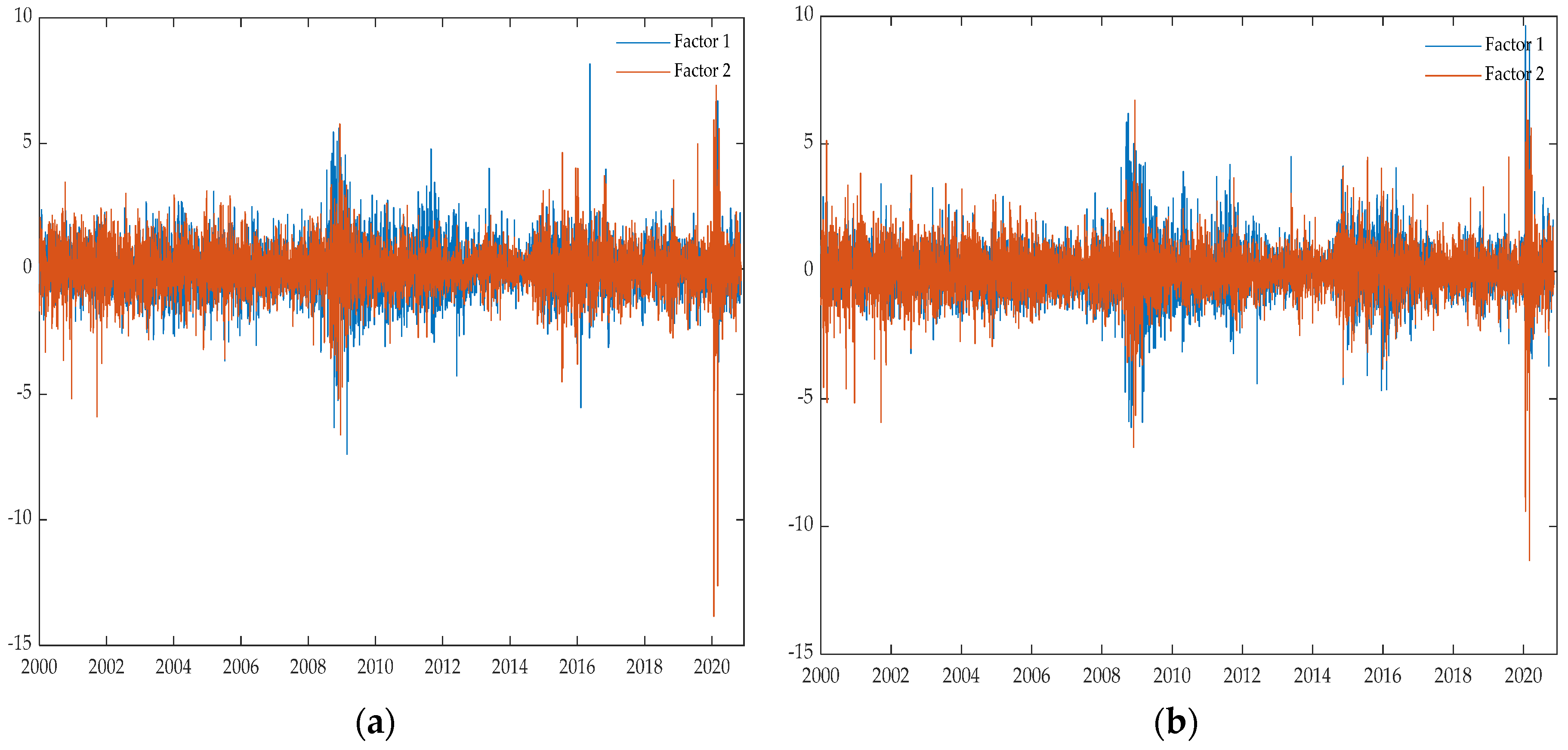
5.1.1. Extraction and Analysis of Common Factors

We first employ the factor analysis to discover the common latent factors in both crude oil and exchange rate returns. Figure 1 presents the “scree plot” of the eigenvalues of the rank correlation matrix of standardized residuals, motivated by the discussion in Section 3.1. The figure shows that the first two eigenvalues are very large, all greater than one, indicating the presence of multiple common factors in the copula. The next one eigenvalue is just above one, while the subsequent eigenvalues become less than one. Taking estimation error into account, we might suspect that only two common factors are needed in our analysis.

Figure 2 depicts the historical evolution of trends for the two common factors related to both crude oil and exchange rate returns. Then we find that the behavior of the common factors has a similar trend with macro-economic indicators over time: in particular, the large fluctuations have been identified in the period from 2008 to 2010, as well as in the year of 2020. Therefore, serious economic impact, such as from the global financial crisis and coronavirus disease 2019 (COVID-19), can lead to the significant volatility of the common factors related to the financial markets. To this end, the extracted common factors can be used to better characterize the overall macro-economic circumstance. These factors can affect the volatility of an individual market as well as the overall interdependence between crude oil and exchange rate markets directly and indirectly. Then we can capture the interdependence among markets and measure the extreme risks more precisely, conditional on the common factors.

5.1.2. Estimation of Marginal Distribution

We can calculate the idiosyncratic factor $Z_i$ related to crude oil and exchange rate returns, respectively, from the residuals to the above two-factor model. The AR-GARCH model is employed to construct the conditional marginal distribution in consideration of autocorrelation and conditional heteroscedasticity, as indicated in Table 1.

Table 2. Parameter estimation of marginal distribution based on AR-GARCH-t model.

	ϕ0	ϕ1	ω	α	β	ν
CNY	−0.004	0.069	0.001	0.036	0.956	9.578
	(0.004)	(0.013)	(0.000)	(0.005)	(0.006)	(1.197)
EUR	0.003	−0.145	0.010	0.052	0.931	11.918
	(0.009)	(0.014)	(0.003)	(0.008)	(0.013)	(1.791)
GBP	0.010	0.086	0.005	0.032	0.959	13.400
	(0.010)	(0.014)	(0.002)	(0.005)	(0.007)	(2.078)
JPY	0.012	−0.042	0.006	0.055	0.929	7.245
	(0.010)	(0.015)	(0.002)	(0.008)	(0.011)	(0.705)
INR	0.012	0.084	0.005	0.047	0.933	11.559
	(0.007)	(0.014)	(0.001)	(0.007)	(0.011)	(1.676)
USDX	0.007	−0.106	0.007	0.039	0.950	7.386
	(0.008)	(0.014)	(0.002)	(0.006)	(0.007)	(0.710)
ZAR	−0.005	-	0.022	0.068	0.913	7.660
	(0.005)		(0.006)	(0.011)	(0.015)	(0.732)
BRL	0.011	−0.016	0.024	0.103	0.872	6.594
	(0.014)	(0.009)	(0.006)	(0.017)	(0.021)	(0.608)
CAD	0.002	−0.061	0.007	0.050	0.934	7.375
	(0.005)	(0.014)	(0.002)	(0.009)	(0.013)	(0.697)
DZD	−0.001	0.013	0.004	0.053	0.937	8.449
	(0.007)	(0.041)	(0.001)	(0.009)	(0.010)	(1.015)
MXN	−0.011	0.004	0.005	0.094	0.896	7.394
	(0.018)	(0.051)	(0.002)	(0.017)	(0.018)	(0.774)
NGN	0.000	−0.094	0.001	0.260	0.740	3.001
	(0.001)	(0.014)	(0.000)	(0.023)	(0.027)	(0.085)
NOK	0.011	−0.059	0.015	0.072	0.904	8.533
	(0.025)	(0.014)	(0.006)	(0.019)	(0.027)	(1.073)
RUB	0.012	−0.006	0.005	0.081	0.908	7.334
	(0.007)	(0.064)	(0.001)	(0.012)	(0.013)	(0.734)
WTI	0.153	−0.039	0.325	0.074	0.910	5.448
	(0.040)	(0.014)	(0.072)	(0.009)	(0.010)	(0.419)
Brent	0.111	−0.076	0.162	0.077	0.915	5.974
	(0.052)	(0.014)	(0.048)	(0.011)	(0.012)	(0.489)

Note: standard errors of the parameters are in parentheses.

presents the estimated coefficients for respective idiosyncratic factors. We find that only the conditional volatility of the exchange rate in South Africa (ZAR) follows an AR (0)-GARCH (1,1)-t process, while other time series can be better fitted with an AR (1)-GARCH (1,1)-t model. The values of the freedom degree of the t-distribution measured by ${\nu }_i$ range from five to thirteen, which indicates that the error terms do not follow normal distribution. The coefficients of the GARCH term as measured by ${\beta }_i$ are positive and close to one, which indicates that the volatility shocks are quite persistent.

5.1.3. Estimation of Time-Varying Factor Copula Model

We try to estimate the parameters and Kendall dependence coefficients of the five typical time-varying copula models based on the empirical results of the conditional distribution for the idiosyncratic factors corresponding to crude oil and exchange rate returns. The respective estimation results are shown in

Table 3. The comparison of the optimal time-varying copulas between the factor copula and Copula–GARCH models.

	Factor Copula Model		Copula–GARCH Model
Model	Kendall	AIC	Kendall	AIC
Panel 1: Exchange rate—WTI
CNY-WTI	0.011	−176.903	−0.036	−62.258
EUR-WTI	0.024	−72.748	−0.066	−140.11
GBP-WTI	0.129	−264.46	−0.094	−201.655
JPY-WTI	−0.242	−1133.3	0.01	−127.041
INR-WTI	0.236	−842.88	−0.029	−32.531
ZAR-WTI	0.095	−224.727	−0.117	−320.095
USDX-WTI	0.056	−111.725	−0.108	−300.123
BRL-WTI	0.05	−102.913	−0.109	−289.389
CAD-WTI	0.348	−1939.5	−0.215	−817.4
DZD-WTI	−0.069	−573.459	−0.077	−178.663
NGN-WTI	0.136	−632.674	−0.01	−17.863
NOK-WTI	0.056	−106.164	−0.149	−444.214
RUB-WTI	0.083	−300.759	−0.132	−410.775
MXN-WTI	−0.048	−72.053	−0.024	−33.459
Panel 2: Exchange rate—Brent
CNY-Brent	0.006	−110.192	−0.03	−45.76
EUR-Brent	0.014	−37.238	−0.063	−19.279
GBP-Brent	0.112	−301.756	−0.091	−194.035
JPY-Brent	−0.246	−608.996	0.017	−128.334
INR-Brent	0.224	−750.27	−0.06	−163.396
ZAR-Brent	0.114	−248.937	−0.106	−281.554
USDX-Brent	0.044	−78.4	−0.102	−272.35
BRL-Brent	0.051	−96.537	−0.103	−224.636
CAD-Brent	0.347	−1943.7	−0.207	−732.936
DZD-Brent	−0.091	−485.298	−0.076	−175.216
NGN-Brent	0.139	−654.972	−0.006	−25.653
NOK-Brent	0.052	−102.782	−0.14	−382.998
RUB-Brent	0.08	−298.88	−0.127	−38.904
MXN-Brent	−0.048	−79.489	−0.022	−35.883

Note: the optimal copula model has been labeled with the smallest AIC value in bold.

. We also compare the results from the factor copula model with the traditional Copula–GARCH model without consideration of their common factors. Furthermore, we compare the dynamic Kendall coefficients from the empirical distribution function (EDF), factor copula model and Copula–GARCH models. Taking China and Brazil as examples, Figure 3 presents the corresponding results about the interdependence between WTI returns and their exchange rate returns, respectively. Then we find that the proposed factor copula model can be considered as the better fitting model than the Copula–GARCH model to capture the dynamic dependence structure of crude oil and exchange rates returns.

We have also found that the constructed time-varying t-copula model is more effective for capturing the dynamic dependence between crude oil and exchange rate markets for most oil-trading countries. Furthermore, the corresponding Kendall dependence is weak for all oil-exchange-rate pairs; nevertheless, the oil exporters’ exchange rates have relatively stronger links with crude oil prices than the oil importers. This finding is almost consistent with the overall sample results of Liu et al. [43]. The higher oil prices can transfer the wealth from oil importers to oil exporters, leading to the devaluation of the currencies of oil importers; however, the currencies of oil exporters will be appreciated instead. Then we identified the positive dependence with exchange rates of oil importers but negative dependence with those of oil exporters.

In addition, the dependence structure has been modified between crude oil and exchange rate returns, conditional on the common factors. For example, compared with the results based on the Copula–GARCH model, the conditional dependence of CAD-OIL and NGN-OIL has been enhanced, while that of NOK-OIL and RUB-OIL has been weakened. Then we can infer that the identified common factors have a great influence on the dependence between their exchange rates and crude oil returns. Especially when some crude macro-economic indicators such as stock market index or consumer confidence index have been changed, the trend in both crude oil and exchange rates would have been affected by the macro-economic circumstance. Therefore, it is necessary to accurately capture the dynamic dependence structure between exchange rates and crude oil markets, conditional on the common factors related to the overall economy.

5.2. Comparison of Dynamic Conditional Dependence

We adopt the estimation results from the factor copula model to calculate the dynamic Kendall dependence coefficients for the conditional dependence among the crude oil and exchange rates of oil importers and exporters, respectively. Then we try to provide a further study on the respective market dependence structure conditional on the common factors. As to the exchange rate of each oil-trading country, the respective conditional dependence structure with WTI returns is almost the same as that with Brent returns during the sample period. Then we just choose the WTI future prices as the representative crude oil prices in the following comparative analysis.

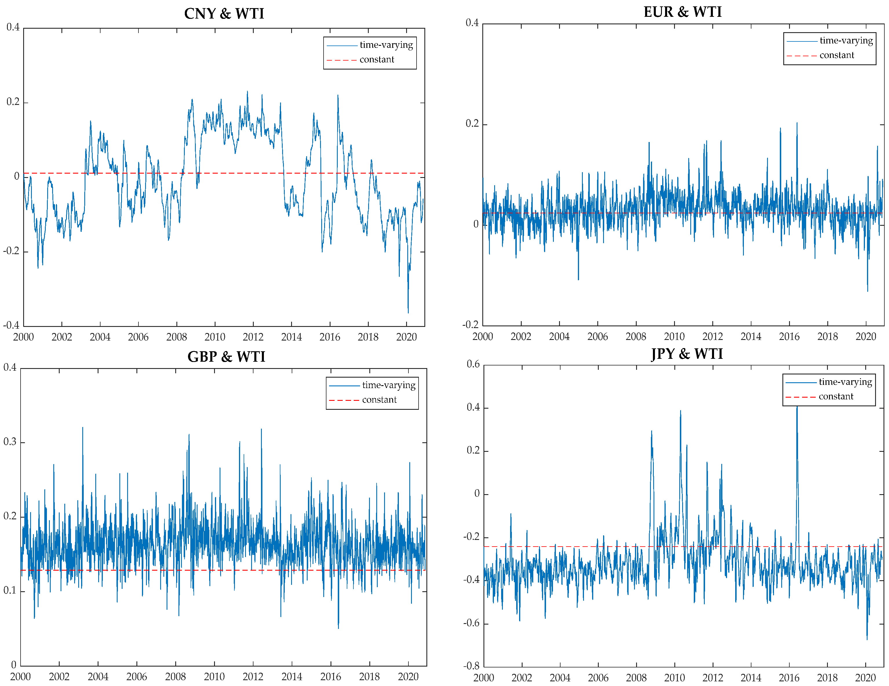
5.2.1. Dynamic Dependence for Oil Importers

Figure 4 illustrates the respective dynamic Kendall dependence between crude oil and exchange rate returns conditional on the common factors, corresponding to each oil importer. We can also compare the time-varying value with their constant dependence. With the increasing financialization of the crude oil markets, the dependence between crude oil and exchange rate returns of oil importers can be characterized by alternative positive and negative values in the full sample period [2]. We also identified the different dependence patterns across the oil importers: as to the INR-OIL pair, it presents a positive dependence degree over time, with a mean value of around 0.3. Subsequently, the EUR-OIL, GBP-OIL and ZAR-OIL pairs exhibit positive dependence with slight fluctuation in all sample periods except during the financial crisis period. Furthermore, the USDX-OIL has also showed the positive dependence within the sample period, because the increase in prices of crude oil is only consistent with a slight appreciation of foreign currency against the USD [44]. In contrast, the exchange rates of other oil importers do not have a continuous positive dynamic correlation with crude oil prices. For example, the dependence coefficient of CNY to oil fluctuations has always been less than zero throughout most of the sample period.

The respective empirical results mean that the idiosyncratic factors related to each time series still have a significant impact on the dependence structure between the crude oil and exchange rate returns of oil importers. Here, we take the CNY/USD exchange rate as an example. China has become the world’s top crude oil importer with continuously increasing oil demand [39]. Compared with the results based on the Copula–GARCH model in Liu et al. [43], the conditional dependence magnitude of the CNY-OIL pair becomes larger, especially after year 2015 when China overtook the United States and became the largest oil importer. We infer that with the rapid development of the economy, China’s demand for crude oil has a progressively significant impact on the volatility of the global oil market price. At the same time, the common factors would impose a relatively slight effect on the dependence among the crude oil prices and the exchange rates of China. Then we can capture the dependence structure among financial markets more precisely, conditional on their common factors.

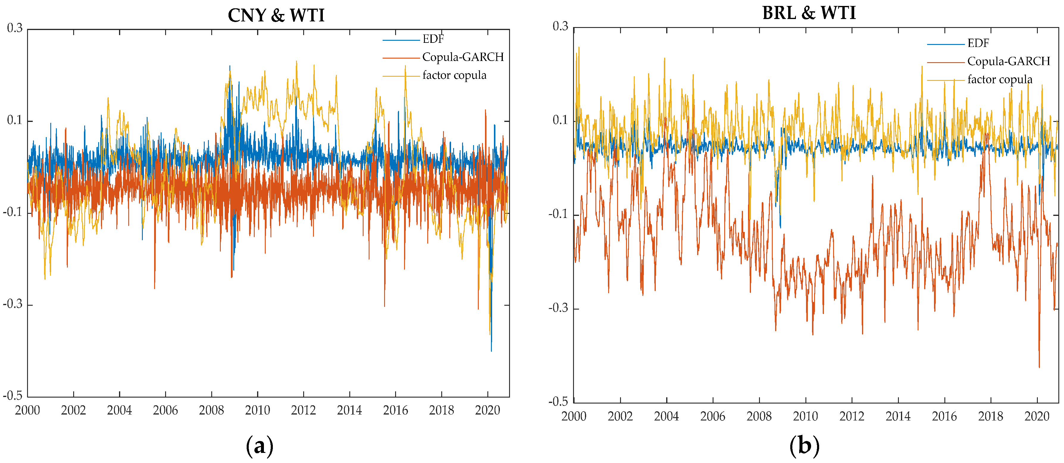
5.2.2. Dynamic Dependence for Oil Exporters

Figure 5 illustrates the respective dynamic Kendall dependence between the crude oil and exchange rate returns of oil exporters, conditional on the common factors. A comparatively stable and small dependence has been captured for the BRL-OIL, NOK-OIL and MXN-OIL pairs over time. In contrast, there is larger dependence as well as greater fluctuations among the dependence of crude oil prices with exchange rates of the remaining oil exporters. Their respective dynamic dependence can also be characterized by alternative positive and negative values over time. However, there is positive dynamic dependence for the CAD-OIL pair in the full sample period. This suggests that the rise of crude oil prices has not always brought about the appreciation of the Canadian currency.

We find that the oil exporters’ conditional dependence characteristics for the oil-exchange-rate pairs are almost the same as in the Copula–GARCH model shown in Liu et al. [43]; nevertheless, we have identified a much larger dependence magnitude between the financial markets in consideration of respective common factors. The factor copula model can capture the relatively greater variation in the market dependence after the 2008 global financial crisis and in the COVID-19 era. Specifically, the Kendall’s τ coefficient for these markets increases significantly during the crisis period but gradually decreases as the crisis effects subside. This indicates that the macro-economic circumstance has played an important role in the relationship of oil exporters’ exchange rates with the crude oil returns, especially during the era of financial crisis. Correspondingly, the dependence of the RUB-OIL pair is almost positive but fell below zero from the years 2012–2016. At this moment, the global economic recovery has driven the demand for oil, leading to the rise of the crude oil price and the appreciation of the Russian currency.

To this end, we have identified the relatively larger conditional dependence magnitude between the crude oil and exchange rate returns of oil-trading countries, in contrast with the results based on the Copula–GARCH model. Specifically, the idiosyncratic factors of oil importers can lead to significant variation in the interdependence among the financial markets. In contrast, the common factors related to the macro-economic circumstances have been identified to play an important role in the variation of volatility dependence between the crude oil and exchange rate markets of the oil exporters.

5.3. Analysis of Dynamic Risk Spillover

We can calculate CoVaR and delta CoVaR for both the exchange rates and crude oil returns based on the optimal time-varying factor copulas at a 95% confidence level ($\alpha =\beta =0.05$), in order to measure the risk spillover between the two markets. We then compare the ∆CoVaR of the exchange rate with that of crude oil returns, conditional on their common factors. The means of the respective dynamic %∆CoVaR are shown in

Table 4. The means of dynamic %∆CoVaR between exchange rate market and crude oil market ($\alpha =\beta =0.05$).

		Relative Magnitude of Risk Spillover from Exchange Rate Markets to Crude Oil Markets		Relative Magnitude of Risk Spillover from Crude Oil Markets to Exchange Rate Markets
		WTI	Brent	WTI	Brent
Oil-importing countries	CNY	0.103%	0.206%	−41.107%	14.314%
	EUR	0.976%	0.487%	25.981%	9.783%
	GBP	5.123%	4.969%	146.462%	108.772%
	JPY	−7.246%	−8.513%	−331.318%	−290.366%
	INR	5.965%	6.485%	376.709%	308.864%
	ZAR	5.208%	7.235%	87.599%	89.676%
	USDX	2.121%	2.143%	63.091%	47.112%
Oil-exporting countries	BRL	2.795%	3.193%	62.474%	52.790%
	CAD	10.111%	11.233%	407.752%	344.033%
	DZD	−1.363%	−2.299%	−132.248%	−122.832%
	NGN	3.026%	2.986%	963.133%	815.145%
	NOK	2.432%	2.602%	67.167%	55.305%
	RUB	2.182%	2.567%	132.785%	116.097%
	MXN	−1.822%	−1.845%	−82.683%	−62.630%

.

We have identified the relatively higher risk spillovers from the crude oil market to the exchange rate market of oil-trading countries. Especially, there is a stronger impact of risk spillover from the crude oil market on the exchange rate of the JPY, INR, CAD and NGN, conditional on the common factors. For example, the risk premium of WTI to CAD and NGN has reached 407.752% and 963.133%, respectively. Only when there is the extreme fluctuation during the economic crashes can the idiosyncratic factors make a substantial contribution to the calculation of the %∆CoVaR. However, in contrast to the results based on the Copula–GARCH model [43], there is almost no conditional risk spillover from the exchange rate market to the crude oil market in the long run.

6. Conclusions

This paper adopted the factor copula model to analyze the non-linear conditional dynamic structure and risk spillovers between crude oil and exchange rate returns. Specifically, we first identified the common factors affecting the returns on both the crude oil prices and exchange rates of 14 typical oil-trading countries. Then we used the AR-GARCH model to filter the respective idiosyncratic factors and conducted a comparative study of the conditional dynamic dependence between the crude oil and exchange rate markets of both oil importers and exporters. Finally, we combined the dynamic factor copula model with the CoVaR method to measure the conditional risk spillover effect between crude oil and exchange rate markets.

The corresponding empirical study suggests the following conclusions: First, the classical factor analysis helps us to precisely identify the common factors related to the financial markets, with a similar trend of macro-economic indicators over time. Second, the factor copula model can capture the dynamic structure between crude oil and ex-change rate markets more accurately than the traditional Copula–GARCH model. Third, the idiosyncratic factor related to each return series still has a significant impact on the dependence between crude oil and exchange rate returns of oil importers, while the common factors have played an important role in the relationship of oil exporters’ exchange rates with crude oil prices. Last but not the least, the crude oil market has enjoyed a relatively higher risk premium to the exchange rate markets of oil-trading countries. In contrast, there is almost no conditional risk spillover from the respective exchange rates to the crude oil price in the long run.

We can provide some useful suggestion for investors, policymakers and exchange rate regulators with further insights from the macro-economic perspective. The respective investors, especially from oil exporters, can first identify the crucial macro-economic factors and then optimize their oil-exchange-rate portfolio strategy in order to deal with the market’s extreme risks more accurately. The oil importers’ macroeconomic policymakers should pay attention to the impact from domestic economic policies on the demand for crude oil and then keep an eye on exchange rates and inflation in the face of the rise in crude oil prices. Differently, the oil exporters should keep a watchful eye on the global economic circumstance and try to flexibly adjust the prices and volume of oil exports, in response to the rapid decrease of the demand for crude oil. Finally, the exchange rate regulators should monitor the effect of risk spillover from the crude oil market to their exchange rate market. They can focus on the currency appreciation risks in case of high oil return shocks. However, they can guard against the risk spillover from the crude oil markets to the currency depreciation when the crude oil prices decrease dramatically.

There are also some potential shortcomings to this study. For example, we can adopted the factor copula model to further analyze the tail conditional dependence between the financial markets and then assessed the downside and upside CoVaRs more precisely. We can also identify the common factors more accurately and then discussed the role of each common factor in the dependence structure of the financial markets. In addition, we will combine the factor analysis with the vine copula model to identify the dynamic dependence among the multiple financial markets.

References

1. Nikbakht, L. Oil prices and exchange rates: The case of OPEC. Bus. Intell. J. 2010, 3, 83–92. [Google Scholar]
2. Beckmann, J.; Czudaj, R.L.; Arora, V. The relationship between oil prices and exchange rates: Revisiting theory and evidence. Energy Econ. 2020, 88, 104772. [Google Scholar] [CrossRef]
3. Albulescu, C.T.; Ajmi, A.N. Oil price and US dollar exchange rate: Change detection of bi-directional causal impact. Energy Econ. 2021, 100, 105385. [Google Scholar] [CrossRef]
4. Hussain, S.I.; Li, S. The dependence structure between Chinese and other major stock markets using extreme values and copulas. Int. Rev. Econ. Financ. 2018, 56, 421–437. [Google Scholar] [CrossRef]
5. Hamdi, B.; Aloui, M.; Alqahtani, F.; Tiwari, A. Relationship between the oil price volatility and sectoral stock markets in oil-exporting economies: Evidence from wavelet nonlinear denoised based quantile and Granger-causality analysis. Energy Econ. 2019, 80, 536–552. [Google Scholar] [CrossRef]
6. Granger, C.W.; Teräsvirta, T.; Patton, A.J. Common factors in conditional distributions for bivariate time series. J. Econ. 2006, 132, 43–57. [Google Scholar] [CrossRef]
7. Huang, S.; An, H.; Lucey, B. How do dynamic responses of exchange rates to oil price shocks co-move? From a time-varying perspective. Energy Econ. 2020, 86, 104641. [Google Scholar] [CrossRef]
8. Golub, S.S. Oil prices and exchange rates. Econ. J. 1983, 93, 576–593. [Google Scholar] [CrossRef]
9. Yang, L.; Cai, X.J.; Hamori, S. Does the crude oil price influence the exchange rates of oil-importing and oil-exporting countries differently? A wavelet coherence analysis. Int. Rev. Econ. Financ. 2017, 49, 536–547. [Google Scholar] [CrossRef]
10. Reboredo, J.C. Modelling oil price and exchange rate co-movements. J. Policy Model. 2012, 34, 419–440. [Google Scholar] [CrossRef]
11. Ahmad, A.; Hernandez, R.M. Asymmetric adjustment between oil prices and exchange rates: Empirical evidence from major oil producers and consumers. J. Int. Financ. Mark. Inst. Money 2013, 27, 306–317. [Google Scholar] [CrossRef] [Green Version]
12. Aloui, R.; Ben Aïssa, M.S.; Nguyen, D.K. Conditional dependence structure between oil prices and exchange rates: A copula-GARCH approach. J. Int. Money Financ. 2013, 32, 719–738. [Google Scholar] [CrossRef]
13. Adrian, T.; Brunnermeier, M.K. CoVaR. Am. Econ. Rev. 2016, 106, 1705–1741. [Google Scholar] [CrossRef]
14. Zhu, D.; Galbraith, J.W. Modeling and forecasting expected shortfall with the generalized asymmetric Student-t and asymmetric exponential power distributions. J. Empir. Financ. 2011, 18, 765–778. [Google Scholar] [CrossRef]
15. Liu, B.-Y.; Ji, Q.; Fan, Y. Dynamic return-volatility dependence and risk measure of CoVaR in the oil market: A time-varying mixed copula model. Energy Econ. 2017, 68, 53–65. [Google Scholar] [CrossRef]
16. Krupskii, P.; Joe, H. Factor copula models for multivariate data. J. Multivar. Anal. 2013, 120, 85–101. [Google Scholar] [CrossRef]
17. Oh, D.H.; Patton, A.J. Modeling Dependence in High Dimensions with Factor Copulas. J. Bus. Econ. Stat. 2017, 35, 139–154. [Google Scholar] [CrossRef]
18. Manner, H.; Manner, H.; Stark, F.; Stark, F.; Wied, D.; Wied, D. Testing for structural breaks in factor copula models. J. Econ. 2018, 208, 324–345. [Google Scholar] [CrossRef]
19. Lin, B.; Su, T. Does oil price have similar effects on the exchange rates of BRICS? Int. Rev. Financ. Anal. 2020, 69, 101461. [Google Scholar] [CrossRef]
20. Hussain, M.; Zebende, G.F.; Bashir, U.; Donghong, D. Oil price and exchange rate co-movements in Asian countries: Detrended cross-correlation approach. Phys. A Stat. Mech. Appl. 2017, 465, 338–346. [Google Scholar] [CrossRef]
21. Tiwari, A.; Trabelsi, N.; Alqahtani, F.; Bachmeier, L. Modelling systemic risk and dependence structure between the prices of crude oil and exchange rates in BRICS economies: Evidence using quantile coherency and NGCoVaR approaches. Energy Econ. 2019, 81, 1011–1028. [Google Scholar] [CrossRef]
22. Guo, R.; Ye, W. A model of dynamic tail dependence between crude oil prices and exchange rates. N. Am. J. Econ. Financ. 2021, 58, 101543. [Google Scholar] [CrossRef]
23. Malik, F.; Umar, Z. Dynamic connectedness of oil price shocks and exchange rates. Energy Econ. 2019, 84, 104501. [Google Scholar] [CrossRef]
24. Benedetto, F.; Mastroeni, L.; Quaresima, G.; Vellucci, P. Does OVX affect WTI and Brent oil spot variance? Evidence from an entropy analysis. Energy Econ. 2020, 89, 104815. [Google Scholar] [CrossRef]
25. Fratzscher, M.; Schneider, D.; Van Robays, I. Oil Prices, Exchange Rates and Asset Prices. ECB Working Paper 2014, No. 1689. Available online: https://ssrn.com/abstract=2442276 (accessed on 1 July 2014).
26. Ledoit, O.; Wolf, M. Improved estimation of the covariance matrix of stock returns with an application to portfolio selection. J. Empir. Financ. 2003, 10, 603–621. [Google Scholar] [CrossRef] [Green Version]
27. Zhang, H.; Jiao, F. Factor Copula Models and Their Application in Studying the Dependence of the Exchange Rate Returns. Int. Bus. Res. 2012, 5, 3. [Google Scholar] [CrossRef] [Green Version]
28. Chen, Z.P.; Song, Z.X. Application of Copula function in coefficient estimation of multi-factor model. Syst. Eng. Theory Pract. 2013, 33, 2471–2478. (In Chinese) [Google Scholar]
29. Song, Q.; Liu, J.; Sriboonchitta, S. Risk measurement of global stock markets: A factor copula-based GJR-GARCH approach. J. Physics: Conf. Ser. 2019, 1324, 012098. [Google Scholar] [CrossRef]
30. Salisu, A.; Mobolaji, H. Modeling returns and volatility transmission between oil price and US–Nigeria exchange rate. Energy Econ. 2013, 39, 169–176. [Google Scholar] [CrossRef]
31. Ding, Q.; Huang, J.; Chen, J. Dynamic and frequency-domain risk spillovers among oil, gold, and foreign exchange markets: Evidence from implied volatility. Energy Econ. 2021, 102, 105514. [Google Scholar] [CrossRef]
32. He, F.; Ma, F.; Wang, Z.; Yang, B. Asymmetric volatility spillover between oil-importing and oil-exporting countries’ economic policy uncertainty and China’s energy sector. Int. Rev. Financ. Anal. 2021, 75, 101739. [Google Scholar] [CrossRef]
33. Zhou, A.M.; Han, F. Research on risk spillover effect between stock market and foreign exchange market: Based on GARCH- time-varying Copula-CoVaR model. Int. Financ. Stud. 2017, 11, 54–64. (In Chinese) [Google Scholar]
34. Lin, J.; Zhao, H. Research on the Risk Spillovers between Shanghai, Shenzhen and Hong Kong Stock Markets-Based on the Time Varying ΔCoVaR Model. System Eng. Theory Pract. 2020, 40, 1533–1544. (In Chinese) [Google Scholar]
35. Chen, T.; Yu, X.L. Measurement of dynamic risk spillover effect in Sino-US cotton futures market: Based on DCC-GARCH-ΔCoVaR model. Pract. Underst. Math. 2021, 51, 282–292. (In Chinese) [Google Scholar]
36. Zhao, R.B.; Tian, Y.X.; Tian, W. Measurement of asymmetric risk spillovers in Financ. markets based on GAS T-Copula model. Oper. Res. Manag. 2021, 30, 176–183. (In Chinese) [Google Scholar]
37. Ji, Q.; Liu, B.-Y.; Fan, Y. Risk dependence of CoVaR and structural change between oil prices and exchange rates: A time-varying copula model. Energy Econ. 2018, 77, 80–92. [Google Scholar] [CrossRef]
38. Patton, A.J. Modelling asymmetric exchange rate dependence. Int. Econ. Rev. 2006, 47, 527–556. [Google Scholar] [CrossRef]
39. Yang, X.Y.; Zheng, Y.H. Application research of fund return dependence based on time-varying Copula model. Econ. Math. 2020, 37, 9–15. (In Chinese) [Google Scholar]
40. Joe, H.; Xu, J.J. The Estimation Method of Inference Functions for Margins for Multivariate Models; Technical Report 166; Department of Statistics, University of British Columbia: Vancouver, BC, Canada, 1996; Available online: http://hdl.handle.net/2429/57078 (accessed on 1 October 1996).
41. British Petroleum. Statistical Review of World Energy, British Pretoleum. 2021. Available online: https://www.bp.com/content/dam/bp/business-sites/en/global/corporate/xlsx/energy-economics/statistical-review/bp-stats-review-2021-all-data.xlsx (accessed on 29 June 2022).
42. International Energy Agency (IEA). Oil Market Report-February 2022; IEA: Paris, France, 2022; Available online: https://www.iea.org/reports/oil-market-report-february-2022 (accessed on 1 February 2022).
43. Liu, B.; Ji, Q.; Nguyen, D.K.; Fan, Y. Dynamic dependence and extreme risk comovement: The case of oil prices and exchange rates. Int. J. Financ. Econ. 2020, 26, 2612–2636. [Google Scholar] [CrossRef]
44. Chen, S.-S.; Chen, H.-C. Oil prices and real exchange rates. Energy Econ. 2007, 29, 390–404. [Google Scholar] [CrossRef]
Figure 1. Scree plots. (a) Scree plot of oil-importing countries. (b) Scree plot of oil-exporting countries.
Energies 15 05220 g001
Figure 2. Dynamic variation characteristics of common factors. (a) Oil-importing countries. (b) Oil-exporting countries.
Energies 15 05220 g002
Figure 3. Dynamic Kendall coefficients of three models for typical countries. (a) CNY-WTI. (b) BRL-WTI. Note: the vertical coordinates correspond to dynamic Kendall coefficients for the respective time-varying dependence between crude oil and exchange rate markets.
Energies 15 05220 g003
Figure 4. Time-varying dependence degree among the crude oil and exchange rates of oil importers. Note: the vertical coordinates correspond to dynamic Kendall coefficients between crude oil and exchange rate returns of each oil importer.
Energies 15 05220 g004aEnergies 15 05220 g004b
Figure 5. Time-varying dependence degree among the crude oil and exchange rates of oil exporters. Note: the vertical coordinates correspond to dynamic Kendall coefficients between crude oil and exchange rate returns of each oil exporter.
Energies 15 05220 g005